Investigating value and growth : what labels hide ?

HAL Id: halshs-00188339

https://halshs.archives-ouvertes.fr/halshs-00188339

Submitted on 16 Nov 2007

HAL is a multi-disciplinary open access archive for the deposit and dissemination of sci-entific research documents, whether they are pub-lished or not. The documents may come from teaching and research institutions in France or abroad, or from public or private research centers.

L’archive ouverte pluridisciplinaire HAL, est destinée au dépôt et à la diffusion de documents scientifiques de niveau recherche, publiés ou non, émanant des établissements d’enseignement et de recherche français ou étrangers, des laboratoires publics ou privés.

Kateryna Shapovalova, Alexander Subbotin

To cite this version:

Kateryna Shapovalova, Alexander Subbotin. Investigating value and growth : what labels hide ?. 2007. �halshs-00188339�

Centre d’Economie de la Sorbonne

Maison des Sciences Économiques, 106-112 boulevard de L'Hôpital, 75647 Paris Cedex 13

http://ces.univ-paris1.fr/cesdp/CES-docs.htm

ISSN : 1955-611X

Investigating Value and Growth : What Labels Hide ?

Kateryna SHAPOVALOVA, Alexander SUBBOTIN 2007.66

Kateryna Shapovalova

, Alexander Subbotin

Abstract

Value and Growth investment styles are a concept which has gained extreme popularity over the past two decades, probably due to its practical efficiency and relative simplicity. We study the mechanics of different factors’ impact on excess returns in a multivariate setting. We use a panel of stock returns and accounting data from 1979 to 2007 for the companies listed on NYSE without survivor bias for clustering, regression analysis and constructing style based portfolios. Our findings suggest that Value and Growth labels often hide important heterogeneity of the underlying sources of risks. Many variables, conventionally used for style definitions, cannot be used jointly, because they affect returns in opposite directions. A simple truth that more variables does not necessarily mean better model nicely summaries our results. We advocate a more flexible approach to analyzing accounting-based factors of outperformance treating them separately before or instead of aggregating.

Key words: Style Analysis, Value Puzzle, Pricing Anomalies, Equity. Classification JEL: E44, G11, E32.

1

This work is a part of research project in Department of Economic Research IXIS CIB -Subsidiary of NATIXIS, the first author thanks Patrick Artus and Florent Pochon for their helpful remarks and suggestions and second authors thanks Thierry Michel for his suggestive ideas.

2

University of Paris-1 Panthéon-Sorbonne, CES and Department of Economic Research IXIS CIB -Subsidiary of NATIXIS, e-mail : kateryna.shapovalova@malix.univ-paris1.fr

3

University of Paris-1 Panthéon-Sorbonne, CES and Higher School of Economics, e-mail: alexander.subbotin@malix.univ-paris1.fr, correspondence to Kateryna Shapovalova and Alexander Subbotin CES/SNRS,MSE,106 bd de L’Hopital, 75647 Paris CEDEX 13. Tel. +33.144.07.82.71

1. Introduction

Since the notions of value and growth were introduced in the academic finance by Rosenberg et al. (1985) and Fama and French (1992, 1993), they remain among the most vague and mysterious not only in the theoretical view, but in the parishioners’ world as well. The introduction of styles into the analysis of stock performance resides on the idea that some characteristics of companies - issuers of stocks can be helpful to understand anomalies of stock returns. By anomalies of stock returns one usually means the incapacity of the classical Capital Asset Pricing Model (CAPM) by Sharpe (1964), Litner (1965), and Black (1972) to accurately explain stock returns premium.

The empirical contradictions of CAPM was widely documented in 1980s and the beginning of 1990s. DeBondt and Thaler (1985) evidence that stocks with low long-term past returns tend to have higher returns prospects. This necessity implies mean-reverting in long-term returns. Jegadeesh and Titman (1993) evidence that stocks with higher premium over the previous year have higher future returns on average. Banz (1981), Basu (1983), Rosenberg et al. (1985), and Lakonishok et al. (1994) documented the dependence of the premium on different companies’ accounting fundamentals. As a result, the simplicity of the CAPM’s assumption of a single risk factor explaining expected returns has been called into question.

Lakonishok et al. (1994) defined value strategies as buying shares having low prices compared to the indicators of fundamental value such as earnings, book value, dividends or cash flow. They classified stocks into “value” or “glamour” on the basis of past growth in sales and expected future growth as implied by the current Earnings-to-Price ratio. Fama and French (1993, 1996) claimed, however, that a three-factor model is capable of explaining most of the pricing anomalies. The baseline Fama and French (1993) three-factor model assumes that the stock returns premium can be represented as a sum of three components due to different factors: the traditional CAPM market beta, company size and book-to-market equity value. These factors describing “value” and “size” according to authors are to be the most significant factors, outside of market risk, for explaining the realized returns of publicly traded stocks. To represent these risks, they constructed two factors: SMB (Small Minus Big) to address size risk and HML (High Minus Low) to address Value risk.

The returns on SMB and HML portfolios tend to be positive in long term, and the presence of positive premium on Value factors is known as “value puzzle”. The existing explanations are based on: (i) rational models of investor behaviour; (ii) different deviations from rational behaviour and market imperfections. Essentially, the first approach tries to find the factors of risk which are priced by the market. Petkova and Zang (2005) find that the conditional market betas of Value stocks covary positively with the expected market risk premium, and that Value stocks are riskier than Growth stocks in bad times when the expected market risk premium is high. The opposite is true for Growth stocks. Hwang and Rubesam (2006) find that in some periods asymmetries in returns can successfully explain the Value premium puzzle. Xing et Zhang (2005) establish a link between style factors and macroeconomic fundamentals. The behaviourist approach supposes bounded rationality and focuses on the way investors extrapolate past performance into the future (Lakonishok et al, 1994 ; La Porta, 1996 ; La Porta et al, 1997).

Fama and French (1996) argue that the three-factor model with SMB and HML factors is sufficient to capture the effect of most of these characteristics, namely earnings/price, cash flow/price, past sales growth, long term and short-term past earnings. Daniel and Titman (1997) suggest that stocks with high book-to-market have high returns due to some reason that has nothing to do with systematic risk. Namely, it is the characteristic (high Book-to-market) rather than the covariance (high sensitivity to HML) that is associated with high returns. Whatever the explanation of the pricing anomalies could be, it is clear that many firm characteristics are helpful to explain the average stock returns. The conclusion in Fama and French (1996) on the omnipotence of the three-factor model is obtained in a CAPM-type framework,

where risk factors are constructed in a univariate setting. Separate portfolios are constructed for each fundamental variable and then they are plugged simultaneously into the market-pricing equation. Given that accounting factors are correlated, it is not surprising that only the portfolio corresponding to the “strongest” factor comes out significant. It does not mean that other variables would add nothing to the explanatory power of the model in a multivariate setting.

In our view the statement that the three-factor model explains the pricing anomalies cannot be correct due to one simple fact that the HML an SML portfolios’ returns are not risk factors themselves, but only proxies for some economic phenomenon. It can only be argued that these proxies are better than others if taken in a univariate setting. The latter does not prove that other variables do not matter if taken simultaneously with Fama and French factors, and especially if the Daniel and Titman’s (1997) argument is true. The ongoing research on the importance of such variables as Earnings-to-Price and Sales growth (Levis and Liodakis, 2001; Park and Lee, 2003; Chan and Lakonishok, 2004; Anderson and Brooks, 2006) evidences that at least not everything is captured by the three-factor model.

Analysing characteristics’ rather than covariances’ explanation power as Daniel and Titman (1997) suggest can indeed be a more direct way of modeling pricing anomalies. The fundamentals themselves rather than HML portfolio returns can be viewed as proxys of some systematic risk factors. This allows for including several indicators simultaneously if they have better explanatory power, which is often done by practitioners. While the academic papers mainly focused on explaining the value puzzle, practitioners did their best to exploit style-based investment strategies. Nowadays all leading index providers compute Value and Growth benchmarks widely used in financial industry. However, the underlying definitions of Value and Growth have undergone a significant evolution. They use multifactor approach with numerous fundamentals to proxy investment styles.

The leading index providers, including Standard&Poor’s (S&P), Morgan Stanley Capital International (MSCI), FTSE Group (FTSE) and STOXX Limited (STOXX), determine the style characteristics of stocks as some combination from a set of the following factors (projected, current and historical):

• Price-to-Earnings ratio: based on the closing price and either on the expected or historical Earnings-per-Share;

• Price-to-Book ratio: based on the closing price and the Book Value-per-Share;

• Price-to-Cash Flow based on the closing price and either on the expected or historical Cash Flow;

• Dividend Yield: based on the closing price at the time of the review and on total dividends declared by the company during the previous 12 months;

• Growth of Earnings-per-Share computed from historical or forecasted data either for long or short term;

• Growth of Sales-per-Share computed from historical or forecasted data either for long or short term;

• Internal Growth which is the portion of Return-on-Equity retained by the company from investment.

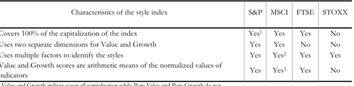
Table 1 summarise the methods used by the leading index providers for attributing stocks to Value and Growth portfolios. Unlike the classical Fama and French (1992) approach, they use several variables to represent both Value and Growth. Moreover, for S&P and MSCI “not value” does not mean Growth: there are two separate dimensions.

Almost all providers use common technique: scoring based on general heuristics without objective function (STOXX Ltd., who uses multivariate clustering). Generally the relative discriminating power of factors is not studied, instead, factors are (almost) identically weighted.

Table 1 Comparison of Methodologies Used for Computing Style Indices

Characteristics of the style index S&P MSCI FTSE STOXX Covers 100% of the capitalization of the index Yes1 _{Yes Yes No}

Uses two separate dimensions for Value and Growth Yes Yes No No Uses multiple factors to identify the styles Yes Yes2 _{Yes Yes}

Value and Growth scores are arithmetic means of the normalized values of

indicators Yes Yes

3 _{Yes No}

1 _{Value and Growth indices cover all capitalisation while Pure Value and Pure Growth do not} 2 _{After 2003}

3 _{Except one indicator for which has been arbitrarily assigned a double weight}

Source: S&P’s Introducing a Comprehensive Style Index Solution: Methodology of S&P’s U.S. Style Indices, may 2005; MSCI Methodology Book: MSCI Index calculation methodology, February 2006; The FTSEGlobal Style Index Series Ground Rules, September 2002; Dow Jones STOXX official website

The performance of style indices by different providers are not similar, which can be explained by the choice of factors and the way they are aggregated. One can judge how good or bad the multifactor definitions are from the performance of indices only, because no cross-sectional analysis of the impact of these factors on performance. Within the rational paradigm method pricing, accounting fundamentals can be considered as proxies of different market risk factors. The number and the nature of the latter are unknown so the effect of using groups of variables to mimic some hidden “Value” or “Growth” factors is dubious. Compared to the mainstream academic research, we make a step “backwards”, concentrating our work on the definitions of styles and pricing anomalies before explaining them.

In our view the study of the value puzzle cannot ignore the issue of accurate style definitions. Initially the choice of the Price-to-Book ratio was justified by the capability of this variable to explain excess return premium. The coherence of other variables should be justified in the same way. Once the impact of accounting fundamentals on the stock performance has been studied, we can start searching for underline factors of market risk. We are mainly interested in multifactor definitions of Value and Growth which enables evaluating the quality of the style indices published by leading providers. Our data includes total returns (dividend yield incorporated) and accounting data for stock quoted on the New York Stock Exchange from 1979 to 2007.

The results of clustering analysis are globally consistent with conventional multifactor style definitions, though cluster patterns are found to evolve in time. However, the link between various accounting indicators and stock performance appears to be more complicated. We signal poor performance of some widely used style scoring schemes which can potentially affect the quality of benchmarks. For example, multifactor definition of Value using Price-to-Book and Price-to-Earnings which seems intuitively plausible is found to be inconsistent and results in unnatural and heterogeneous data aggregation. Besides, the use of growth of Earnings-per-Share (historical or forecasted) is very ambiguous. We identify several variables which influence stock returns permanently and study how these effects are interrelated. This analysis is the first step in tackling the style puzzle.

The rest of the work is organised as follows. The next section starts with the results of clustering analysis based on accounting variables. It is followed by section 3 describing regressions of stock returns on these variables. Section 4 presents a number of portfolios designed with use of the definitions of Value and Growth factors. We finally overview the main results and suggest directions for further research.

2. Clustering by Style Factors

We start by clustering stocks according to different financial ratios without incorporating market returns. Such analysis determines categories of stocks which are “naturally close” according to some definition of distance. However, clustering is based on variables which do the best to separate stocks into different groups but not necessarily indicators which are influence market returns considerably. Therefore, we continue by building regression models for excess returns with financial ratios used as predictors. Finally, we construct several portfolios using previous results on Value and Growth factors in order to explicitly characterise their performance.

Clustering analysis is a way to create a group of objects (clusters) such as the profiles of objects in the same cluster are very similar, and the profiles of objects in different clusters are as distinct as possible. We use the so-called K-means clustering method. A short summary of the clustering theory used in this section can be found in Mirkin (2005). What we call the profile is a multi-dimensional vector of financial ratios which are used to describe the company issuer of the stock.

While choosing candidates for Value and Growth factors we were largely inspired by the existing literature and index providers’ style definitions. Potential Value factors are ratios of some accounting measures of past or projected performances to the current market price. Book Value represents the wealth of company accumulated from all of its past performances while Cash Flow, Sales and Earnings account for company’s results of the previous year. If these ratios are high company’s growth prospects are poorly valuated by investors, if they are low, on the contrary, investors’ consensus is optimistic. Potential Growth factors are represented by the increase in Earnings, Sales and Dividend-per-Share computed over different historical periods or forecasted, completed by the Internal Growth measure which is the portion of the reinvested Return on Equity. Other variables include measure of size (Market Capitalisation) and Beta which estimates the sensibility of stock to movements of the market.

All data is pre-processed using the probability integral transform which enables mapping on to comparable scale ranging from zero to one. Thus we do not consider absolute values of indicators but the relative ranking. A detailed description of variables and information on their availability can be found in Appendix 1.

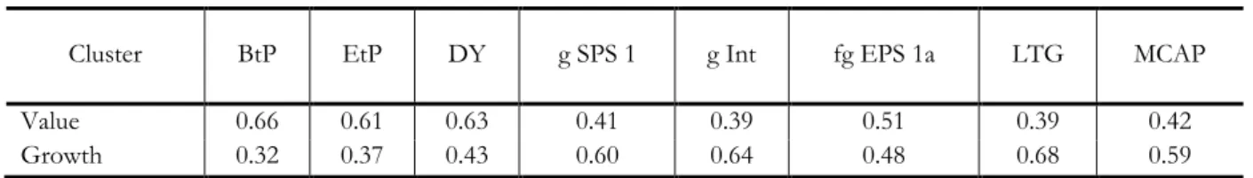
We start by splitting the universe of stocks into two groups using all available data set from 1984 to 2006. Table 2 represents the mean values of the best-separating indicators for each cluster. First cluster can easily be identified as Value: both Book-to-Price and Earning-to-Price are above 0.5 and Dividend Yield is higher than average. On the contrary all conventional Growth measures (growth of Sales-per-Share, Internal Growth, forecasted growth of Earnings-per-Share for the next fiscal year and Long Term Growth forecast) are lower than average. The stocks in this cluster have lower Market Capitalisation and Beta. The other cluster can apparently be labelled Growth.

Table 2 Two-cluster Model for Value and Growth, years 1984-2006

Cluster BtP EtP DY g SPS 1 g Int fg EPS 1a LTG MCAP Value 0.66 0.61 0.63 0.41 0.39 0.51 0.39 0.42 Growth 0.32 0.37 0.43 0.60 0.64 0.48 0.68 0.59

K-means clustering, values of financial ratios in cluster centres. Computation by the authors.

This result is generally consistent with a multifactor approach to style classification adopted by the index providers. Conventional Value factors are concertedly higher in one cluster then in the other and Value is most likely not Growth. The stability of clusters in time was tested by breaking the period of analysis into two parts: prior and after 1996. These results are available from the authors on request.

The quality of data separation by clustering can be judged by the distances between stocks within and out of the clusters represented graphically by the silhouette plot (Figure 1). The silhouette value ranges from one for stocks which are close to points in their own cluster but fare from points in other clusters, through zero for stocks which are not distinctly form one cluster to another, to minus one for probably incorrectly assigned stocks. The plot to the left of Figure 1 refers to clustering based on all data set (from 1984 to 2006). We can observe that the Value cluster is less homogeneous than the Growth cluster this is mainly due to period 1996-2005 as can be seen on the silhouette plots in the centre and to the right of Figure 1 which correspond respectively to the sub-periods prior and after 1996. This means that style clusters evolve in time with Value becoming less clear-cut.

Figure 1 Silhouette Plot of Two-cluster Model for all Period, and Two Sub-periods Prior and Post 1996

Silhouette values on the x-axis and percentage of stocks in Value and Growth on y-axis for the periods 1984-2006 (to the left), 1984-1995 (in the middle) and 1996-2006 (to the right)

This evidence is supported by clustering into three and four groups. A three clusters model is non-stable in time: for the first sub-period we find traditional Value and Growth clusters and a group of stocks with small Market Capitalization and all conventional Value and Growth measures varying around 0.5 so they cannot be assigned to either of the styles. For the second sub-period the new cluster corresponds to stocks with high Dividend Yield, modest growth prospects and medium values of Book-to-Price and Earnings-to-Price ratios lower than average. We call such stocks “Elephants”.

The results of four-cluster model are more suggestive (Table 3, 4, 5). Clustering on the whole data set results in four groups of stocks whose characteristics allow rather straightforward interpretations: conventional Value stocks have high Book-to-Price and Earnings-to-Price ratios and low Growth indicators. Conventional Growth stocks have inverse characteristics. Dividend Yield is roughly similar for the two clusters. The so-called “Elephants” class subsists. Stocks in the other group have Book-to-Price higher than average and Earnings-to-Price lower than average, low Dividend Yield and good earnings growth prospects according to analysts’ forecast, which are, however, not supported by current growth of sales. Beta of these stocks is the highest compared to all the other three clusters. We call these promising but intuitively risky stocks “Tigers”. It is interesting that they tend to look overvalued in terms of book value but not current earnings as compared to market price.

Table 3 Four-cluster Model for Value and Growth, all dataset period

Cluster BtP EtP DY g SPS 1 g Int fg EPS 1a LTG MCAP Value 0.71 0.79 0.48 0.51 0.60 0.37 0.53 0.34 Tigers 0.62 0.30 0.43 0.42 0.27 0.64 0.59 0.32 Elephants 0.53 0.59 0.81 0.41 0.36 0.56 0.26 0.61 Growth 0.24 0.34 0.43 0.64 0.71 0.45 0.70 0.66

The results for the sub-periods show that the described above structure is more characteristic for the later period: for years 1984-1995, Elephants and Tigers cannot be well distinguished, while for the subsequent period the profiles become sharper.

Table 4 Four-cluster Model for Value and Growth, years 1984-1995

Cluster BtP EtP DY g SPS 1 g Int fg EPS 1a LTG MCAP

Value 0.66 0.64 0.80 0.42 0.39 0.50 0.29 0.64

No Style I 0.67 0.47 0.36 0.41 0.46 0.32 0.60 0.27

No Style II 0.53 0.47 0.55 0.78 0.41 0.63 0.59 0.32

Growth 0.24 0.44 0.37 0.49 0.68 0.54 0.55 0.69

K-means clustering, values of financial ratios in cluster centres. Computation by the authors.

Overall, the results of clustering analysis demonstrate that a two-cluster vision of styles is oversimplified. More precisely, Book-to-Price, Earnings-to-Price and Dividend Yield are not always coherent for defining Value, and historical growth does not always act in the same sense as the forecast of earnings.

Table 5 Four-cluster Model for Value and Growth, years 1996-2005

Cluster BtP EtP DY g SPS 1 g Int fg EPS 1a LTG MCAP Value 0.71 0.79 0.49 0.51 0.60 0.36 0.52 0.35 Tigers 0.62 0.31 0.44 0.39 0.25 0.64 0.61 0.35 Elephants 0.50 0.56 0.81 0.44 0.37 0.54 0.25 0.58 Growth _{0.24 0.34 0.45 0.62 0.71 0.49 0.70 0.67}

K-means clustering, values of financial ratios in cluster centres. Computation by the authors.

For the more recent period along with conventional Value and Growth we were able to identify groups of stocks which are characterised by highly divergent style measures: Tigers with high Book-to-Price ratio, but low Earnings-to-Book-to-Price ratio, low current growth of Sales-per-Share and high expected Earnings Growth rate; Elephants with average Book-to-Price and Earnings-to-Price, and very high Dividend Yield. Potentially, this can lead to less accurate results of multifactor style models. However, we have no idea on whether the clusters are homogeneous in terms of the impact of the underlined indicators on market performance. This motivates the regression analysis presented in the following section.

3. The Effects of Style Factors on Performance

The idea behind assigning stocks to Value and Growth portfolios emerges from the finding that some accounting fundamentals such as Book-to-Price and Earnings-to-Price are helpful to explain the part of excess return premium which is not captured by beta in traditional CAPM model. Therefore, any definition of styles using multiple variables should be justified by the ability of these variables to forecast returns. For each year from 1984 to 2006 we estimated regressions of stock performances on a set of chosen factors described in details in Appendix 1. Like in clustering analysis, all factors were transformed in ranks and scaled between zero and one. This makes our results less sensitive to outliers.

Along with a large number of candidates for Value and Growth factors we include a measure of size which is the Market Capitalisation of the company, and Beta which is estimated according to Cunningham (1973). These variables are used as controls for estimating the impact of Value and Growth factors in accordance with the tree-factor model approach. First we estimate an ordinary least squares regression model with returns quantile as dependant variable. We have run several regressions consecutively eliminating insignificants and unstable factors. The final results are presented in Table 6. For

robustness purposes, we also estimate a logit model for the probability of the given stock to outperform the market. It is rendered by the binary variable taking the value one if the annual total return was higher than median return for the market and zero otherwise using logit regression. It did not alter the results significantly. Detailed reports are available from the authors on request.

To ensure that the accounting indicators were publicly available to investors before the returns are recorded we use a lag of five months from the nominal date to which those indicators refer. So accounting data prior to 31 December of year t is used to predict the change in price from 1st _{June year t+1 to 1}st _June

year t+2. This makes our estimates conservative given that if accounting information were available before the 1st _{June, it could at least partially be reflected in price prior to this date.}

For Value factors we find that the traditional Fama and French factor Book-to-Price is most often significant for explaining returns. The effect is positive for 20 years of 22 almost always statistically significant. As we can see in Table 6, according to the results of OLS regression, there is one period for which the effect of Book-to-Price ratio was negative and significant: 1998. For the rest of the years the effect is positive and quite important (except 2004). The results of the logit regression are generally similar to those of the OLS.

For Earnings-to-Price ratio we obtain less stable results, both when it is included in regression together with Book-to-Price and when the latter is excluded. The coefficient are not as often significant, and when they are, their signs are unpredictable and do not match with those of Book-to-Price coefficients. In the latest period (2002-2005) high Book-to-Price yields high returns while high Earnings-to-Price decreases returns, all other factors kept constants. Therefore these two factors can hardly be combined for defining Value. For the Cash Flow-to-Price we do not observe such strange behaviour, higher Cash Flow-to-Price tends to reinforce the effect of higher Book-to-Price. For the Sales-to-Price ratio, the results are almost similar to those for Earnings-to-Price: regression coefficients are rarely significant and their signs switch. This is probably due to the fact that typical value of Sales-to-Price varies largely across economic sectors, depending on the average profit margins so the Sales-to-Price variable might reflect the changes in relative performance in sectors with different profit margins.

The effect of Dividend Yield, which is often used to define value, tends to be positive and significant at the same years as the Book-to-Price before 1992, but for the later period this coherence vanishes. The ratio is driven by both changes in Dividends-per-Share and Price. Apparently the role of dividends has evolved since the 90th with the appearance of classes of companies which abstained from paying dividends for the long periods. This probably led to the distortion of the effect of Dividend Yield on expected performance.

These findings suggest that the usage of multifactor models for defining Value in most cases is not justified by data. Except Cash Flow-to-Price all other variables do not add much to the prediction given by Book-to-Price ratio and even counterbalance it. Such conclusions are mainly derived from the recent 10 years data which is supported by the evidence on the evolution of the style clusters. Probably, the Tigers and Elephants do not really share the same investor attitude as traditional Value stocks.

As regards Growth factors the results are even more intriguing. First we find a huge discrepancy between the impacts on returns by the historical and forecasted growth measures. Among the forecasted growth indicators a one year forward growth rate of Earnings-per-Share is significant for all years in the sample, except for the last year, with the negative sign. This could be explained by the overreaction of the markets to the news provided by the financial analysts. The price of stocks with promising prediction jumps shortly after the forecasts are published (and before the date from which we start computing returns which is the 1st June of each year). The initial rise can be followed by a slung when investors become aware that the stock is overvalued. This effect is probably captured in regression. For the Long Term Growth consensus the conclusion is similar though the significance of its effect on return is lower.

The impact of the dispersion of growth consensus is ambiguous: it is positive for some years and negative for the other.

Table 6 Ordinary Least Square Regression on Permanent Factors

Year Const BtP CFtP g SpS 1 fg EPS 1a Beta R2

1985 0.37 0.15 N/A 0.26 -0.43 0.05 0.10 (5.22***) (2.29**) (4.11***) (-6.63***) (0.82) 1986 0.19 0.12 N/A 0.12 -0.12 -0.23 0.05 (3.63***) (2.42**) (2.47**) (-2.58**) (-4.8***) 1987 -0.02 0.15 N/A 0.07 -0.13 -0.14 0.06 (-0.41) (4.12***) (2.02**) (-3.52***) (-3.77***) 1988 0.23 0.09 N/A 0.12 -0.25 0.04 0.06 (4.99***) (2**) (2.94***) (-5.49***) (0.9) 1989 0.15 0.05 N/A 0.26 -0.36 -0.04 0.03 (1.52) (0.61) (3***) (-3.92***) (-0.51) 1990 0.17 0.06 N/A 0.13 -0.24 -0.01 0.04 (3.04***) (1.24) (2.7***) (-4.7***) (-0.12) 1991 0.10 0.27 0.04 0.15 -0.28 -0.02 0.06 (1.57) (4.86***) (0.78) (2.87***) (-4.96***) (-0.45) 1992 0.02 0.31 0.1 0.29 -0.21 -0.04 0.07 (0.33) (5.38***) (1.59) (5.21***) (-3.41***) (-0.72) 1993 0.00 0.10 0.07 0.11 -0.18 0.08 0.05 (0) (2.61***) (1.73*) (2.91***) (-4.46***) (2.2**) 1994 0.02 0.11 0.11 0.16 -0.18 0.05 0.04 (0.34) (2.41**) (2.38**) (3.66***) (-3.66***) (1.16) 1995 0.29 0.09 -0.02 0.23 -0.26 0.13 0.02 (2.91***) (1.16) (-0.24) (2.88***) (-3.01***) (1.54) 1996 0.10 0.21 0.22 0.09 -0.24 -0.03 0.08 (2.05**) (5.4***) (5.04***) (2.45**) (-5.72***) (-0.86) 1997 0.18 0.26 0.12 0.15 -0.31 0.06 0.08 (3.22***) (6.07***) (2.46**) (3.48***) (-6.48***) (1.28) 1998 0.15 -0.14 0.14 0.13 -0.4 -0.03 0.06 (2.4**) (-2.69***) (2.47**) (2.54**) (-7.41***) (-0.52) 1999 0.07 0.09 0.14 -0.11 -0.44 0.25 0.07 (1.06) (1.63) (2.38**) (-1.99**) (-7.73***) (4.43***) 2000 0.02 0.51 0.19 0.19 -0.17 -0.16 0.07 (0.25) (8.65***) (2.96***) (3.29***) (-2.63***) (-2.65***) 2001 0.08 0.47 -0.08 0.04 -0.24 -0.12 0.1 (1.45) (10.56***) (-1.55) (0.85) (-5.04***) (-2.68***) 2002 0.03 0.08 0.06 0.10 -0.17 -0.15 0.02 (0.48) (1.73*) (1.17) (2.39**) (-3.67***) (-3.33***) 2003 0.12 0.37 0.08 0.03 -0.15 0.14 0.03 (1.45) (5.55***) (1.05) (0.52) (-2.07**) (2.02**) 2004 0.04 0.21 0.11 0.21 -0.21 -0.06 0.06 (0.91) (5.51***) (2.69***) (5.59***) (-5.26***) (-1.6) 2005 -0.14 0.21 0.07 0.25 -0.10 0.13 0.05 (-2.83***) (5.04***) (1.62) (5.98***) (-2.19**) (3.03***) 2006 0.13 0.06 0.01 0.04 0.00 -0.01 0.00 (2.93***) (1.65*) (0.35) (0.97) (-0.08) (-0.21)

Cross-sectional OLS regression for each year, the difference between stock return and All Market return is used as dependant variable. All factors (see Appendix 1) are transformed to uniform scale (form 0 to 1). T-statistics are reported in parentheses below the coefficient estimates. T-statistics significant at 1% level are marked by ***, at 5% level are marked by **, at 10% level are marked by *. Source: Datastream, 5,194stocks quoted on NYSE, years 1979-2007.

The historical growth of Earnings-per-Share has relatively low insignificant and often negative effect on returns. At the same time historical growth of Sales-per-Share appears to be a better indicator. Its impact is positive and significant for almost all year. Surprisingly, computing growth over longer historical period (three and five years instead of one year) does not significantly improve the results. Hence, the performance of Growth portfolio can be easily manipulated by the choice of growth measure: it suffices to take historical Growth of Sales to obtain an outperforming index or forecast of earnings

growth to fall below the benchmark. The highest performance is expected for the stocks having low expected earnings forecast relatively to historical growth of sales.

4. Construction of Style-based Portfolios

We proceed by constructing various portfolios based on factors described above in order to explicitly characterise their performance, designing a number of style portfolios based on different Value and Growth factors. All of them are weighted by Market Capitalisation in order to represent some fixed portions of the market, which is arbitrary fixed at the level of 25% for all style portfolios. Performance of all stocks is measured by total return including dividends. The composition of each style basket is updated every year on the 1st _{of June using accounting data on the 31 December for the previous year. The}

performance of these portfolios is compared to internal benchmark representing a Market Capitalisation weighted average of all the stocks in database for which data is available.

The results for each model are represented in Tables 7-18. The tables present yearly returns and summarise the main quantitative performance measures for Value, Growth, No Style and All Market portfolios. All statistics are computed for the whole sample (23 years), two subsamples (the same as for clustering analysis) prior and after 1996, and the resent 5 years. We compute nine indicators using raw total returns and three indicators relative to the benchmark (All Market). The indicators measuring performance in absolute terms include annualised returns, volatility, Sharpe ratio, maximum drawdown, beta, portion of systematic and specific risk, skewness and kurtosis of return’s distribution. Indicators of relative performance are: annualised outperformance, tracking error and relative maximum drawdown.

The first model uses Book-to-Price ratio as the only discriminating variable with stocks having high Book-to-Price assigned to Value and low Book-to-Price assigned to Growth. Another one-factor model uses Earnings-to-Price instead of Book-to-Price. They are somewhat like benchmark models, borrowing ideas from Fama and French (1992) and Basu (1983), Ball (1978) respectively. Table 7 represents the performance of Value and Growth portfolios in the model based on Book-to-Price ratio and Table 8 summarise the main quantitative performance measures.

Table 7 Performance of Portfolios Constructed with Price-to-Book Ratio

A

bs

ol

ut

e

All Market No Style Growth Value

R el at iv e to A ll M ar k et Value Growth 1985 33,0 37,7 30,3 31,1 -1,9 -2,8 1986 34,3 33,3 24,9 39,5 5,3 -9,4 1987 0,6 -2,5 2,2 1,0 0,4 1,5 1988 25,4 21,9 24,2 31,7 6,3 -1,2 1989 36,9 29,5 50,2 35,2 -1,7 13,3 1990 1,6 3,9 9,0 -7,5 -9,1 7,4 1991 32,8 29,2 46,4 28,7 -4,1 13,6 1992 24,5 20,4 17,3 34,3 9,7 -7,3 1993 15,0 21,6 -3,6 21,6 6,6 -18,6 1994 3,1 2,5 2,1 2,4 -0,7 -1,0 1995 42,4 42,2 44,6 46,2 3,9 2,3 1996 30,6 35,9 30,8 28,7 -2,0 0,2 1997 38,1 40,3 38,8 37,0 -1,1 0,7 1998 27,6 15,7 39,8 19,3 -8,3 12,1 1999 26,1 19,3 29,7 18,6 -7,5 3,6 2000 20,6 20,6 6,5 31,0 10,4 -14,1 2001 6,8 15,2 0,0 14,8 8,0 -6,8 2002 -3,0 7,1 -9,3 4,3 7,3 -6,3 2003 23,6 30,2 10,9 31,6 8,0 -12,7 2004 20,4 19,4 10,0 27,4 7,0 -10,4 2005 16,8 21,9 11,2 23,6 6,8 -5,6 2006 18,9 21,0 14,3 21,4 2,5 -4,7

Annual returns of style portfolio (in %). Computation by the authors. Source: Datastream, 4540 stocks quoted on NYSE, years 1979-2007.

The Value portfolio defined by high Book-to-Price considerably outperforms (five percents or more) the market in 1986, 1988, 1992-1993 and 2000-2005. These results are not strictly equivalent to those obtained for the coefficients before the Book-to-Price factor in the regression described above because the latter is estimated in multivariate setting, all other factors equal while in the univariate setting portfolio construction we suffer from all sources of multi-colinearity.

However, the basic trends are the same: high outperformance in 1992-1993 and 2000-2005. It is interesting that in 2001 the relative return does not go below zero though the regression coefficient was significant. As can be seen in Table 8, the annualised outperformance is 2.04 %, and this figure is largely due to recent years’ good results. The Sharpe ratio, which represents expected return on one unit of standard deviation, is 1.33 for the whole period and 2.02 for the recent five years. Note that the increase in outperformance in the last years was accompanied by decreasing volatility.

Table 8 Performance Measures for the Portfolios Constructed with Price-to-Book Ratio

T im e p eri o d s 1 A bs ol ut e A n n u al iz ed R et u rn , % V o la ti lit y, % S h arp e R at io M ax D ra w d o w n , % B et a S ys te m at ic R is k, % S p ec if ic R is k, % S ke w n es s K u rt o si s R el at iv e to A ll M ar k et A n n u al iz ed O u tp erf o rm an ce , % M ax R el at iv e D ra w d o w n , % T ra ck in g E rro r, % V al u e 1 ₂ 23.16 _22.80 13.74 _13.73 1.33 -24.59 0.96 _{1.22 -24.59 0.93 88.81} 88.06 _11.19 11.94 _-0.99 -0.58 _8.66 6.28 _0.99 2.04 _-14.32 -16.16 4.77 _4.71 3 23.47 13.80 1.62 -16.75 1.01 87.72 12.28 -0.20 4.13 3.04 -14.38 4.83 4 24.41 10.74 2.02 -8.44 1.06 93.23 6.77 -0.45 3.89 5.27 -1.64 2.86 G ro w th 1 ₂ 18.60 _21.17 15.04 _15.77 0.91 -28.22 1.02 _{0.96 -28.22 1.05 86.71} 82.47 _13.29 17.53 _-0.76 -0.22 _7.18 5.75 _-0.62 -2.50 _-27.81 -50.32 6.30 _5.79 3 16.19 14.33 1.05 -22.58 0.98 77.85 22.15 0.44 4.03 -4.18 -43.30 6.75 4 13.13 8.98 1.16 -8.73 0.79 74.35 25.65 -0.24 2.96 -5.79 -27.94 4.97 N o S ty le 1 21.68 14.24 1.18 -25.06 1.01 90.41 9.59 -0.42 6.04 0.57 -22.81 4.41 2 20.94 13.58 1.10 -25.06 0.94 94.14 5.86 -0.92 7.38 -0.85 -17.34 3.38 3 22.35 14.89 1.42 -20.11 1.09 88.41 11.59 -0.06 5.12 1.93 -16.98 5.20 4 22.09 11.16 1.74 -8.03 1.09 90.06 9.94 -0.22 3.74 3.00 -3.46 3.62 A ll M ark et 1 21.11 13.38 1.21 -26.57 1.00 100.00 0.00 -0.61 7.18 2 21.80 13.97 1.13 -26.57 1.00 100.00 0.00 -1.16 9.68 3 20.41 12.84 1.29 -17.75 1.00 100.00 0.00 0.06 3.95 4 19.03 9.75 1.67 -8.75 1.00 100.00 0.00 -0.58 3.73

1_{1- years 1985-2005; 2- years 1984-1995; 3- years 1996-2007; 4- years 2002-2007}

Computation by the authors. Source: Datastream, 5,194 stocks quoted on NYSE, years 1979-2007.

As it could be expected, the outperformance of Growth portfolio is an almost symmetrical reflection of Value outperformance around zero axes. Nevertheless, the drawdowns and the upturns are more abrupt and of higher amplitude. Indeed, the maximum drawdown in absolute terms was -28.22% against-24.59% for the Value in absolute terms and -50.32% against -16.60% for Value in relative terms. The portion of specific risk for this portfolio is much higher than for Value. It goes up to 25.65% for the recent five years compared to 6.77% for Value. The Beta of the Growth portfolio decreased from 1.05 during the first subsample to 0.79 during last five years. So the sharp fluctuations of the Growth portfolio are mainly explained by higher specific risk.

The model constructed with Earnings-to-Price as measure for Value appears to be significantly different for the previous model (Table 9, Table 10). The performance of Value portfolio is quite comparable to the one defined by Book-to-Price except that it has lower outperformance for the years in the first subsample and higher for the years 2000-2001, 2005. The overall annualised outperformance is 2.31%, a little higher than for the previous model, and 4.32% for the recent five years i.e. almost 1% lower. Interestingly, the Earnings-to-Price ratio is rarely reported significant in the multivariate regression setting,

driven out by other variables. Meanwhile, for univariate portfolio construction the preference between Book-to-Price and Earnings-to-Price for definition of Value cannot be easily established.

Table 9 Performance of Portfolio Constructed with Price-to-Earnings Ratio

A

bs

ol

ut

e

All Market No Style Growth Value

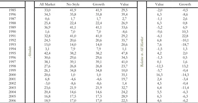
R el at iv e to A ll M ar k et Value Growth 1985 33,0 41,9 41,9 29,5 -2,0 -0,5 1996 34,3 35,8 35,8 39,4 6,3 -8,6 1987 0,6 1,7 1,7 2,7 -1,1 2,6 1988 25,4 22,4 22,4 26,9 6,3 0,8 1989 36,9 41,1 41,1 33,6 -5,2 6,9 1990 1,6 7,0 7,0 -8,6 -9,6 10,3 1991 32,8 41,0 41,0 29,2 -6,1 22,8 1992 24,5 20,6 20,6 35,7 6,8 -10,1 1993 15,0 14,0 14,0 20,6 7,6 -18,7 1994 3,1 7,9 7,9 1,1 -1,5 1,3 1995 42,4 38,2 38,2 47,8 4,2 2,0 1996 30,6 29,6 29,6 34,5 -1,3 0,5 1997 38,1 39,1 39,1 41,0 0,1 1,6 1998 27,6 26,8 26,8 23,7 -12,3 13,2 1999 26,1 34,8 34,8 10,0 -5,7 -0,4 2000 20,6 1,0 1,0 35,1 16,3 -14,3 2001 6,8 -4,6 -4,6 19,7 2,4 -3,4 2002 -3,0 -8,6 -8,6 1,4 4,5 -0,4 2003 23,6 21,9 21,9 32,7 6,4 -11,4 2004 20,4 14,6 14,6 24,2 5,5 -6,3 2005 16,8 17,5 17,5 28,9 6,3 -6,3 2006 18,9 17,0 17,0 22,5 4,6 -6,2

Annual returns of style portfolio (in %). Computation by the authors. Source: Datastream, 4540 stocks quoted on NYSE, years 1979-2007.

The price of Growth portfolio evolves in opposite direction to the price of Value portfolio, meanwhile it differs from the Growth defined in the previous model. Unlike in the previous model, it does not have significant drawdowns before 2000. On the contrary, the Internet bubble shock affected this portfolio rather significantly leading to relative drawdown 35.85%.

Table 10 Main Performance Measures of the Portfolios Constructed withPrice-to-Earnings Ratio

T im e p eri o d s 1 A bs ol ut e A n n u al iz ed R et u rn , % V o la ti lit y, % S h arp e R at io M ax D ra w d o w n , % B et a S ys te m at ic R is k, % S p ec if ic R is k, % S ke w n es s K u rt o si s R el at iv e to A ll M ar k et A n n u al iz ed O u tp erf o rm an ce , % M ax R el at iv e D ra w d o w n , % T ra ck in g E rro r, % V al u e 1 ₂ 23.43 _22.21 13.73 1.35 -20.46 0.93 _{13.54 1.19 -20.46 0.89} 82.43 _{84.92 15.08} 17.57 -0.14 _-0.46 4.90 _{5.58 0.40} 2.31 _-15.33 -18.39 5.83 _5.47 3 24.57 13.96 1.68 -14.81 0.98 80.68 19.32 0.13 4.35 4.13 -18.39 6.14 4 23.44 11.22 1.85 -10.57 1.03 79.43 20.57 -0.44 5.04 4.32 -5.59 5.10 G ro w th 1 ₂ 20.13 _23.80 16.11 0.94 -35.61 1.13 _{15.92 1.12 -30.49 1.11} 88.85 _94.34 11.15 _{5.66 -1.17} -0.42 6.93 _10.0 -0.98 _1.99 -35.85 _-8.37 5.67 _4.07 3 16.66 16.30 0.95 -35.61 1.16 84.16 15.84 0.26 4.70 -3.71 -35.85 6.82 4 17.42 11.10 1.33 -10.84 1.09 91.27 8.73 -0.44 3.31 -1.58 -8.73 3.39 N o S ty le 1 18.95 14.28 0.98 -28.39 1.02 91.12 8.88 -0.48 6.93 -2.15 -39.35 4.26 2 18.22 14.73 0.83 -28.39 1.02 94.20 5.80 -1.02 9.04 -3.54 -30.67 3.56 3 19.45 13.88 1.32 -20.33 1.01 87.99 12.01 0.14 4.44 -0.95 -15.78 4.81 4 16.14 10.42 1.29 -11.33 1.03 92.39 7.61 -0.70 4.80 -2.83 -11.41 2.89 A ll M ark et 1 21.11 13.38 1.21 -26.57 1.00 100.00 0.00 -0.61 7.18 2 21.80 13.97 1.13 -26.57 1.00 100.00 0.00 -1.16 9.68 3 20.41 12.84 1.29 -17.75 1.00 100.00 0.00 0.06 3.95 4 19.03 9.75 1.67 -8.75 1.00 100.00 0.00 -0.58 3.73

1_{1- years 1985-2005; 2- years 1984-1995; 3- years 1996-2007; 4- years 2002-2007}

Interestingly, Growth basket has positive outperformance of almost 2% over first ten years (-0.62% for the first model), so on average Value and Growth portfolios in Earnings-to-Price model both outperform All Market in the first subsample. In the second subsample, the Growth is below zero, but not as low as in the previous model. In the Price-to-Book model the negative and positive performances of two indices compensate each other so that the All Market and No Style portfolio are essentially the same, in the Earnings-to-Price we find the evidence of non-linearity of returns.

The non-linearity hypothesis is supported by the performance of the No Style portfolio which falls significantly below market. It means that stocks with Earnings-to-Price ratio close to median are worth than stocks in both tails. Our finding explains why this indicator was insignificant in linear regression: two tails are compensating one another. These results are in line with the ideas evoked in clustering analysis section: high Book-to-Price was found to be associated both to high Earnings-to-Price in the traditional value cluster but also with very low Earnings-to-Price in the so-called “Tigers” cluster.

For the subsequent models which use multiple factors for Value and Growth an aggregation technique is needed to obtain the final score. One way could be to compute the arithmetic average. However, this approach is problematic because it does not account for the form of the joint distribution of Growth and Value factors. So using arithmetic average means ignoring information about the correlation structure and hence, losing some important information on the joint distribution of factors.

In a univariate setting the rank of each stock divided by total number of stocks represents the empirical probability of the event that the corresponding indicator lays below the observed value, which is in fact an estimate of the cumulative distribution function (CDF). In presence of several factors, it would be natural to generalize the approach by computing multivariate CDF which represents the probability of the event that the factors fall below some given values simultaneously. But the estimation of multivariate CDF is very complicated since the factors have different scales and very few observations are available for extreme points.

Though, an efficient way of modelling interdependence between variables is to estimate copulae for Growth and Value factors which is based on ranks of indicators rather than on their values. Copula is a function which enables construction of multivariate probability from a set of univariate distributions (Sklar, 1959). Copulae completely describe dependence structure between two or more random variables. They are scale-independent measures depending on the ranks of indicators (marginal CDFs) rather than their raw values. The calibration of copula consists in, first, choosing the family of copulae and then estimating its parameters. In the context of our study the Student copula is most appropriate because it offers enough flexibility to fit the data, being at the same time a rather parsimonious model to estimate in a multivariate setting.

Figure 7 illustrates the difference between computing scores with arithmetic mean and copulae for two factors. The x-axis corresponds to the mean of the factors and the y-axis is the standard deviation, z-axis represents the value of the final score. The upper plot corresponds to positively correlated factors (ߩ = 0.7), the middle plot to independent factors, and the last one to the situation when they are negatively correlated ߩ = −0.7. The arithmetic means scores are situated on the plane since they do not depend on the standard deviation of factor values. For any given value of the mean the copula score decreases with standard deviation. For the strongly correlated factor the two techniques yield almost similar results, as correlation goes down to minus one the surface becomes more convex.

Figure 2 Using copula approach for scoring factors

ߩ = 0.7 ߩ = 0 ߩ = −0.7

The difference between computing scores with arithmetic mean and copulae for two factors. The x-axis corresponds to the mean of the factors and the y-axis is the standard deviation, z-axis represents the value of the final score. The upper plot corresponds to positively correlated factors (ߩ = 0.7), the middle plot to independent factors, and the last one to the situation when they are negatively correlated ( ߩ = −0.7).

The multifactor scoring allows to define not only Value and Growth portfolios but also so-called “Low Value” and “Low Growth” which contain stocks with low Value scores and low Growth scores respectively. If factors used to define Value and Growth are not the same, then Low Value will not necessarily be similar to Growth and Low Growth to Value. If copula technique is used than the Low Value and Low Growth baskets will include stocks for which either all factors are low or their dispersion is high.

The first multifactor model we construct uses three factors for Value (Book-to-Price, Earning-to-Price and Dividend Yield) and three factors for Growth (one year forecast of growth of Earnings-per-Share, Long Term Growth and growth of Sales-per-Share over the last five years). It is intended to proxy the construction of Style definitions by the leading index providers.

Table 11 Performance of Portfolios Constructed Using Three-factor Model

A

bs

ol

ut

e

All Market No Style Growth Value Low Value Low Growth R el at iv e to A ll M ar k et

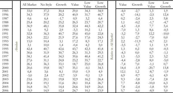
Value Growth Low Value Low Growth 1985 33,0 37,2 30,4 29,0 34,3 34,9 -4,0 -2,7 1,3 1,9 1996 34,3 37,9 20,2 40,9 31,7 46,7 6,7 -14,1 -2,5 12,4 1987 0,6 6,4 -1,7 0,9 3,2 6,4 0,2 -2,4 2,5 5,8 1988 25,4 20,2 25,2 26,5 23,7 20,7 1,1 -0,2 -1,7 -4,7 1989 36,9 48,1 35,8 32,4 44,5 42,2 -4,5 -1,0 7,7 5,4 1990 1,6 9,2 2,9 -5,3 10,2 1,1 -7,0 1,3 8,6 -0,5 1991 32,8 36,3 40,7 29,6 45,0 22,8 -3,2 7,9 12,2 -10,0 1992 24,5 22,1 21,9 27,6 17,6 24,5 3,1 -2,7 -7,0 0,0 1993 15,0 10,4 3,1 17,2 8,3 17,1 2,2 -11,9 -6,7 2,1 1994 3,1 10,0 1,4 -0,4 4,2 5,0 -3,5 -1,7 1,1 1,9 1995 42,4 40,7 42,6 43,7 42,3 41,8 1,3 0,2 0,0 -0,5 1996 30,6 31,9 30,7 26,3 31,3 29,5 -4,3 0,0 0,7 -1,1 1997 38,1 41,4 34,5 39,6 40,4 41,2 1,5 -3,5 2,3 3,2 1998 27,6 31,1 24,8 23,2 35,7 22,7 -4,4 -2,8 8,0 -5,0 1999 26,1 36,3 33,1 18,7 25,0 26,8 -7,4 7,0 -1,1 0,7 2000 20,6 19,8 18,7 35,1 -0,1 34,5 14,4 -1,9 -20,7 13,8 2001 6,8 3,6 8,1 19,0 -1,9 4,9 12,1 1,2 -8,7 -1,9 2002 -3,0 2,4 -12,7 3,9 -9,1 1,9 6,9 -9,7 -6,1 4,9 2003 23,6 20,1 19,8 32,9 16,2 26,4 9,3 -3,8 -7,4 2,8 2004 20,4 19,1 11,6 28,1 10,4 26,7 7,7 -8,8 -10,0 6,3 2005 16,8 16,7 14,4 24,6 14,9 26,6 7,8 -2,4 -1,8 9,9 2006 18,9 14,9 12,4 24,7 10,1 23,9 5,7 -6,6 -8,9 5,0

Annual returns of style portfolio (in %). Computation by the authors. Source: Datastream, 4540 stocks quoted on NYSE, years 1979-2007.

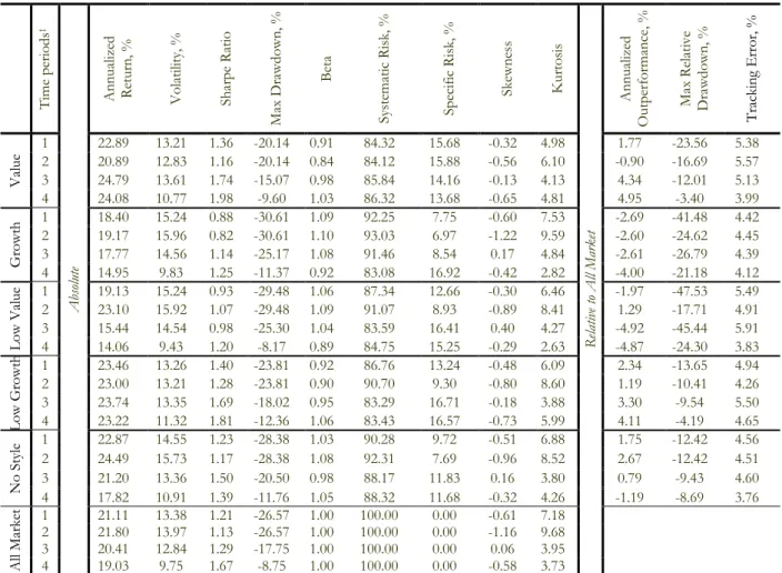
We can see in Table 11 that the performance of the Value portfolio is very instable. For the years 1985-1999 the portfolio has only once outperformed the market by more than 5% (in 1986). For all other years during this period the portfolio followed the market with insignificant fluctuations around zero outperformance. The millennium is marked by a sharp rise of excess return on Value which goes up to 15% above the market. The outperformance sustains afterwards decreasing successively to 5% in 2006.

Most striking is the heterogeneity of the Value outperformance curve before and after 2000. As evidence Table 12, during the subperiod prior to 1996 the annualised outperformance was - 0.90%, while for the later subperiod it is 4.34% and for the last five years even more: 4.95%. Interestingly the growth in relative returns is accompanied by decreasing volatility: it was 12.83% before 1996 and only 10.77% for the recent five years. It makes us think again about possible changes in style patterns, which probably occurred during last decade.

Table 12 Main Performance Measures of the Portfolios Constructed Using Three-factor model.

T im e p eri o d s 1 A bs ol ut e A n n u al iz ed R et u rn , % V o la ti lit y, % S h arp e R at io M ax D ra w d o w n , % B et a S ys te m at ic R is k, % S p ec if ic R is k, % S ke w n es s K u rt o si s R el at iv e to A ll M ar k et A n n u al iz ed O u tp erf o rm an ce , % M ax R el at iv e D ra w d o w n , % T ra ck in g E rro r, % V al u e 1 ₂ 22.89 _20.89 13.21 _12.83 1.36 _1.16 -20.14 _-20.14 0.91 _{0.84 84.12} 84.32 _15.88 15.68 _-0.56 -0.32 _6.10 4.98 _-0.90 1.77 _-16.69 -23.56 5.38 _5.57 3 24.79 13.61 1.74 -15.07 0.98 85.84 14.16 -0.13 4.13 4.34 -12.01 5.13 4 24.08 10.77 1.98 -9.60 1.03 86.32 13.68 -0.65 4.81 4.95 -3.40 3.99 G ro w th 1 ₂ 18.40 _19.17 15.24 _15.96 0.88 _0.82 -30.61 _-30.61 1.09 _{1.10 93.03} 92.25 _6.97 7.75 _-1.22 -0.60 _9.59 7.53 _-2.60 -2.69 _-24.62 -41.48 4.42 _4.45 3 17.77 14.56 1.14 -25.17 1.08 91.46 8.54 0.17 4.84 -2.61 -26.79 4.39 4 14.95 9.83 1.25 -11.37 0.92 83.08 16.92 -0.42 2.82 -4.00 -21.18 4.12 L o w V al u e 1 19.13 15.24 0.93 -29.48 1.06 87.34 12.66 -0.30 6.46 -1.97 -47.53 5.49 2 23.10 15.92 1.07 -29.48 1.09 91.07 8.93 -0.89 8.41 1.29 -17.71 4.91 3 15.44 14.54 0.98 -25.30 1.04 83.59 16.41 0.40 4.27 -4.92 -45.44 5.91 4 14.06 9.43 1.20 -8.17 0.89 84.75 15.25 -0.29 2.63 -4.87 -24.30 3.83 L o w G ro w th _{1 23.46 13.26 1.40 -23.81 0.92 86.76 13.24 -0.48 6.09 2.34 -13.65 4.94} 2 23.00 13.21 1.28 -23.81 0.90 90.70 9.30 -0.80 8.60 1.19 -10.41 4.26 3 23.74 13.35 1.69 -18.02 0.95 83.29 16.71 -0.18 3.88 3.30 -9.54 5.50 4 23.22 11.32 1.81 -12.36 1.06 83.43 16.57 -0.73 5.99 4.11 -4.19 4.65 N o S ty le 1 22.87 14.55 1.23 -28.38 1.03 90.28 9.72 -0.51 6.88 1.75 -12.42 4.56 2 24.49 15.73 1.17 -28.38 1.08 92.31 7.69 -0.96 8.52 2.67 -12.42 4.51 3 21.20 13.36 1.50 -20.50 0.98 88.17 11.83 0.16 3.80 0.79 -9.43 4.60 4 17.82 10.91 1.39 -11.76 1.05 88.32 11.68 -0.32 4.26 -1.19 -8.69 3.76 A ll M ark et 1 21.11 13.38 1.21 -26.57 1.00 100.00 0.00 -0.61 7.18 2 21.80 13.97 1.13 -26.57 1.00 100.00 0.00 -1.16 9.68 3 20.41 12.84 1.29 -17.75 1.00 100.00 0.00 0.06 3.95 4 19.03 9.75 1.67 -8.75 1.00 100.00 0.00 -0.58 3.73

1_{1- years 1985-2005; 2- years 1984-1995; 3- years 1996-2007; 4- years 2002-2007}

Model constructed with three factors for Value: Book-to-Price, Earning-to-Price and Dividend Yield, and three factors for Growth: one year forecast of growth of Earnings-per-Share, Long Term Growth and Growth of Sales-per-Share over the last five years. Computation by the authors. Source: Datastream, 5,194 stocks quoted on NYSE, years 1984-2007.

The Growth portfolio fluctuates in inverse directions compared to its Value counterpart. The recent period is characterised by relative losses amounting down to 10% in 2002. The average outperformance of the portfolio is rather stable for both subperiods and ranges between -2.6% and -2.7% but fell significally to -4% in last five years.. The recent five years are also characterised by decreasing volatility: 9.83% against 15.96% prior to 1996.

The Low Value portfolio is almost a reflection of the Value relative to zero axis, but with slightly higher amplitude of excess returns and losses. It has higher volatility than Value but roughly the same as Growth. It outperforms in almost the same periods as the Growth portfolio but its excess return is usually higher than that of Growth: in 1991 Low Value is 12% while Growth is only 8% above market. In 1998 the Low Value portfolio is the only one to outperform by 8% while the Growth portfolio is slightly below the benchmark and outperforms only in 1999 by 7%.

The pair Growth-Low Growth is characterised by higher asymmetry than the pair Value -Low Value, which means that the structure of underlined dependencies is rather possibly non-linear. In 1998-1999 trends of excess returns on Growth and Low Growth almost coincide. The Low Growth and Value are not really synchronised: in the subperiod before 1996 the annualised outperformance of Low Growth is 1.19% while Value is – 0.99% below the market. On the contrary for the latter subperiod the Low Growth outperforms by 3.30% against 4.34% for Value. Note that Low Growth companies have suffered in 2001 while Value stocks did not.

This overview of three-factor model shows that periods of under and outperformance are rather brief and unsustainable, except maybe the recent blossom for Value. The latter can be explained by high positive return on the Dividend Yield factor at the time when high dividends became rare, combined with positive input of Earnings-to-Price in 2000. Our previous results demonstrate that the factors used for style definitions often influence returns in opposite directions. Therefore the overall impact depends on which variable “pulls” stronger. Remember that the impact of Earnings-to-Price factor, for instance, became negative since 2004 according to the regression results.

The next series of models use a definition of Value by Book-to-Price and Cash Flow-to-Price whose impact on returns was not market by much ambiguity according to the regression results. When Cash Flow-to-Price is unavailable (years 1984-1989) only Book-to-Price is used for the definition. For the Growth we use either a combination of one year forecasted growth of Earnings-per-Share and forward Long Term Growth; historical growth of Earnings-per-Share, or historical growth of Sales-per-Share. Table 13 Performance of Multifactor Model Constructed Using Price-to-Book and Cash Flow-to-Price for Value and forecasted growth of Earnings-per-Share and Long Term Growth for Growth

A

bs

ol

ut

e

All Market No Style Growth Value _Value Low _Growth Low

R el at iv e to A ll M ar k et

Value Growth _Value Low _Growth Low 1985 33,0 33,8 25,6 31,1 30,3 35,1 -1,9 -7,4 -2,8 2,0 1996 34,3 35,2 14,6 39,5 24,8 46,5 5,2 -19,7 -9,4 12,2 1987 0,6 7,4 -4,8 0,9 2,2 9,4 0,3 -5,4 1,5 8,8 1988 25,4 17,9 22,3 31,7 24,2 21,6 6,3 -3,2 -1,2 -3,8 1989 36,9 52,3 32,1 34,2 50,2 40,3 -2,7 -4,7 13,3 3,4 1990 1,6 11,9 -1,9 -7,3 9,0 1,6 -8,9 -3,5 7,4 0,0 1991 32,8 38,5 35,8 26,7 45,7 28,8 -6,1 3,0 12,9 -4,0 1992 24,5 18,3 23,8 28,5 14,8 24,2 3,9 -0,7 -9,8 -0,4 1993 15,0 5,3 3,4 23,6 3,2 20,7 8,6 -11,6 -11,8 5,7 1994 3,1 3,2 2,7 7,3 0,0 3,7 4,2 -0,4 -3,1 0,6 1995 42,4 43,8 37,8 43,4 43,0 46,1 1,1 -4,6 0,6 3,7 1996 30,6 35,0 23,7 37,7 28,8 32,5 7,1 -6,9 -1,8 1,9 1997 38,1 46,5 29,9 40,7 36,2 45,0 2,6 -8,2 -1,9 6,9 1998 27,6 36,7 18,5 25,6 37,1 29,3 -2,0 -9,2 9,4 1,7 1999 26,1 35,2 16,1 19,6 26,1 28,7 -6,5 -10,0 0,0 2,7 2000 20,6 16,1 8,6 30,1 8,0 28,7 9,5 -12,1 -12,7 8,1 2001 6,8 3,8 0,1 7,8 2,7 11,4 0,9 -6,7 -4,2 4,6 2002 -3,0 4,0 -13,2 2,9 -6,9 4,5 5,9 -10,2 -3,9 7,5 2003 23,6 17,7 22,3 35,2 18,0 24,0 11,6 -1,3 -5,6 0,4 2004 20,4 22,0 13,6 27,1 13,5 31,3 6,7 -6,8 -6,9 10,9 2005 16,8 17,9 11,7 20,7 12,4 30,8 4,0 -5,1 -4,3 14,1 2006 18,9 15,8 12,9 23,8 13,7 24,3 4,9 -6,0 -5,2 5,3

Annual returns of style portfolio (in %). Computation by the authors. Source: Datastream, 4540 stocks quoted on NYSE, years 1979-2007.

Adding Cash Flow-to-Price to the Value definition slightly improves the overall results for the Value portfolio, compared to the one-factor Book-to-Price and Earnings-to-Price models, boosting outperformance in 1996-1997and 2003, cutting the loss in 1998-1999. Since 1991 the portfolio has only once been below the market for the period 1998-1999 and the drawdown was not so important as for the previous models. Its annualised outperformance over the whole period was 2.38% with 0.67% prior to 1996, 3.98% after 1996 and 6.10% in the recent five years. The main tendencies such as growth of Beta and reduction of the specific risk and volatility for the latest period are the same as for the one-factor Book-to-Price portfolio.

Table 14 Main Performance Measures of the Portfolio Constructed Using Price-to-Book and Cash Flow-to-Price for Value and forecasted growth of Earnings-per-Share and Long Term Growth for Growth T im e p eri o d s 1 A bs ol ut e A n n u al iz ed R et u rn , % V o la ti lit y, % S h arp e R at io M ax D ra w d o w n , % B et a S ys te m at ic R is k, % S p ec if ic R is k, % S ke w n es s K u rt o si s R el at iv e to A ll M ar k et A n n u al iz ed O u tp erf o rm an ce , % M ax R el at iv e D ra w d o w n , % T ra ck in g E rro r, % V al u e 1 ₂ 23.50 _22.47 14.39 _13.70 1.29 _1.20 -24.59 _-24.59 1.00 _{0.92 88.02} 87.35 _11.98 12.65 _-1.01 -0.51 _8.66 6.01 _0.67 2.38 _-16.82 -16.82 5.12 _4.87 3 24.42 15.07 1.54 -17.41 1.10 88.28 11.72 -0.15 4.25 3.98 -10.91 5.33 4 25.26 11.32 1.99 -9.14 1.12 93.06 6.94 -0.51 4.01 6.10 -2.43 3.21 G ro w th 1 ₂ 14.87 _16.46 15.40 _15.67 0.65 _0.66 -32.02 _-30.21 1.09 _{1.07 91.68} 89.82 10.18 _{8.32 -1.21} -0.55 _9.07 6.65 _-5.29 -6.21 _-40.27 -70.57 5.06 _4.64 3 13.52 15.17 0.82 -32.02 1.11 88.14 11.86 0.13 4.31 -6.83 -51.45 5.41 4 15.37 10.98 1.15 -12.56 1.07 89.76 10.24 -0.43 3.36 -3.58 -17.59 3.57 L o w V al u e 1 19.09 15.02 0.94 -28.22 1.04 85.62 14.38 -0.28 5.87 -2.02 -44.93 5.72 2 21.27 15.73 0.97 -28.22 1.05 87.01 12.99 -0.77 7.21 -0.52 -25.26 5.71 3 17.15 14.33 1.12 -21.25 1.02 84.22 15.78 0.30 4.24 -3.23 -35.10 5.70 4 15.20 9.07 1.38 -9.40 0.87 86.78 13.22 -0.46 3.07 -3.76 -19.98 3.54 L o w G ro w th 1 25.35 13.19 1.55 -22.08 0.92 86.69 13.31 -0.29 5.69 4.22 -7.01 4.94 2 24.33 13.24 1.38 -22.08 0.90 89.37 10.63 -0.66 8.00 2.51 -7.01 4.55 3 26.15 13.17 1.90 -14.52 0.94 84.43 15.57 0.08 3.48 5.69 -6.94 5.25 4 24.97 11.13 2.00 -10.55 1.00 76.34 23.66 -0.56 5.06 5.82 -3.80 5.41 N o S ty le 1 22.83 14.57 1.23 -26.87 1.01 86.19 13.81 -0.35 6.06 1.71 -18.60 5.42 2 23.27 15.47 1.11 -26.87 1.04 88.76 11.24 -0.82 7.21 1.46 -18.60 5.22 3 22.23 13.69 1.54 -15.94 0.97 83.31 16.69 0.29 4.25 1.81 -12.44 5.60 4 18.17 9.54 1.62 -10.03 0.92 88.12 11.88 -0.54 4.96 -0.84 -8.00 3.38 A ll M ark et 1 21.11 13.38 1.21 -26.57 1.00 100.00 0.00 -0.61 7.18 2 21.80 13.97 1.13 -26.57 1.00 100.00 0.00 -1.16 9.68 3 20.41 12.84 1.29 -17.75 1.00 100.00 0.00 0.06 3.95 4 19.03 9.75 1.67 -8.75 1.00 100.00 0.00 -0.58 3.73

1_{1- years 1985-2005; 2- years 1984-1995; 3- years 1996-2007; 4- years 2002-2007}

Computation by the authors. Source: Datastream, 5,194 stocks quoted on NYSE, years 1979-2007.

The definition of Growth which uses the combination of two forecasts yields surprisingly stable results in terms of downperformance: only once has the Growth portfolio been above zero –in 1991 (Table 13). The volatility is slightly higher than for Value but comparable. Average excess loss is -6.21% for the whole period (see Table 14). Maximum relative drawdown reaches -70%. Naturally, the Low Growth portfolio offers positive excess returns which are almost twice as important as the Value. This explains why the No Style portfolio permanently outperforms the market.

The second definition of Growth (Table 15) using historical growth of Earnings-per-Share, a variable often used in style definitions, seems to have very poor discriminating power in according to regression results. Significant outperformance was recorder only in 1991 and 1999. The outperformance of this portfolio is weak and quite stochastic which means that model captures some residual effects coming from correlations with other, really significant factors (Table 16).

Table 15 Performance of Alternative Models for Growth

A bs ol ut e Growth(1) Low Growth(1) Growth(2) Low Growth(2) R el at iv e to A ll M ar k et Growth(1) Low Growth(1) Growth(2) Low Growth(2) 1985 36,5 38,9 38,6 27,3 3,4 5,9 5,6 -5,7 1996 34,4 39,9 36,3 37,1 0,1 5,7 2,0 2,8 1987 -0,2 -2,6 4,6 4,1 -0,9 -3,2 3,9 3,4 1988 24,2 28,2 27,1 25,3 -1,2 2,8 1,7 -0,1 1989 36,0 28,8 41,0 37,7 -0,9 -8,0 4,1 0,8 1990 -1,7 4,5 9,6 -7,4 -3,3 2,9 8,0 -9,0 1991 47,6 19,1 46,6 18,8 14,8 -13,7 13,8 -14,0 1992 19,7 22,9 24,3 26,7 -4,8 -1,6 -0,3 2,2 1993 14,1 18,1 13,3 19,3 -0,9 3,1 -1,7 4,4 1994 0,2 6,7 8,5 5,8 -2,9 3,6 5,4 2,7 1995 43,5 38,7 50,4 40,4 1,1 -3,6 8,0 -1,9 1996 34,0 27,8 41,3 21,6 3,4 -2,8 10,6 -9,0 1997 42,1 33,9 43,7 25,1 4,0 -4,2 5,6 -12,9 1998 24,8 22,9 35,5 20,2 -2,8 -4,7 7,9 -7,4 1999 32,8 12,7 29,9 15,8 6,7 -13,4 3,9 -10,3 2000 12,3 26,6 29,5 18,2 -8,3 6,0 8,9 -2,4 2001 5,0 8,5 9,6 0,4 -1,8 1,7 2,8 -6,4 2002 -8,9 -1,9 -7,5 -2,9 -5,9 1,0 -4,6 0,1 2003 26,4 22,8 23,3 29,6 2,8 -0,8 -0,3 6,0 2004 21,5 21,8 28,4 22,7 1,1 1,5 8,0 2,3 2005 19,8 13,9 26,2 16,8 3,0 -2,8 9,4 0,0 2006 22,1 21,2 20,1 21,8 3,2 2,3 1,2 2,8

Annual returns of style portfolio (in %). Growth (1) and Low Growth (1) are constructed using growth of Earnings-per-Share, Growth (2) and Low Growth (2) are constructed with growth of Sales-per-Share. Computation by the authors. Source: Datastream, 4540 stocks quoted on NYSE, years 1979-2007.

Finally, the definition of Growth by historical dynamics of Sales-per-Share (Table 15), chosen on the basis of regression and clustering result, yields the results consistent with our expectations. The excess return is slightly below zero for 1993 and 2002 only, for the rest of the sample it outperforms the market.

As reported in Table 16 the overall annualised outperformance is 4.40% which is almost twice as high as Value. For the recent five years, however, Value does better than Growth: 6.10% against 3.71%. Except for these recent years, the Growth has slightly lover volatility, so that the Sharpe ratios are roughly similar (1.33 for Growth and 1.29 for Value). For the first subsample Growth is more aggressive with Beta 1.11 compared to 0.92 for Value, while for the recent years the situation is opposite: 1.12 for Value and 0.98 for Growth. The latter became less predictable with specific risk increasing sharply from 6.36% in the first subsample to 16.08% most recently (for the Value the tendency was inverse). This is probably due to the new emerging economic activities of the digital era where growth of sales does not have the same meaning as for traditional economic sectors.

Counter-intuitively, Growth and Value do not seem to be antagonistic: though some hedging effect is present, especially in 1988-1991 and 1999, they often outperform simultaneously. So combining Value and Growth produces a well hedged portfolio, biting the market during all the sample period.