The emerging aversion to inequality - Evidence from long subjective data

HAL Id: halshs-00586788

https://halshs.archives-ouvertes.fr/halshs-00586788

HAL is a multi-disciplinary open access archive for the deposit and dissemination of sci-entific research documents, whether they are pub-lished or not. The documents may come from teaching and research institutions in France or

L’archive ouverte pluridisciplinaire HAL, est destinée au dépôt et à la diffusion de documents scientifiques de niveau recherche, publiés ou non, émanant des établissements d’enseignement et de recherche français ou étrangers, des laboratoires

The emerging aversion to inequality - Evidence from

long subjective data

Irena Grosfeld, Claudia Senik

To cite this version:

Irena Grosfeld, Claudia Senik. The emerging aversion to inequality - Evidence from long subjective data. 2009. �halshs-00586788�

WORKING PAPER N° 2008 - 19

The emerging aversion to inequality

Evidence from long subjective data

Irena Grosfeld Claudia Senik

JEL Codes: C25, D31, D63, I30, P20, P26

Keywords: inequality, subjective well-being, growth, breakpoint, transition

P

-

S

E

L

’E

A

-

48,BD JOURDAN –E.N.S.–75014PARIS TÉL. :33(0)143136300 – FAX :33(0)143136310

www.pse.ens.fr

The emerging aversion to inequality:

Evidence from long subjective data

Irena Grosfeld

(Paris School of Economics, CNRS), grosfeld@pse.ens.fr

Claudia Senik

(Paris School of Economics, University Paris-Sorbonne, IZA and Institut Universitaire de France), senik@pse.ens.fr,

First version: June 2006

This version: January 2009

We thank Malgorzata Kalbarczyk for outstanding research assistance and Jolanta Sommer for help with the data. We are grateful to Katia Zhuravskaya for insightful comments. We have benefited from discussions with Marc Gurgand, Andrew Clark, and seminar participants in London, Bonn and Paris. The support of CEPREMAP is gratefully acknowledged.

Abstract

This paper provides evidence of a change in the relationship between individual satisfaction with the state of country’s economy and income inequality during transition from a command to market economic system. Using data from a series of extensive and frequent surveys of Polish population, we identify a structural break in this relationship. In the beginning of transition, an increase in income inequality is interpreted by population as a positive signal of increased opportunities; this sentiment is particularly strong among older people and people with right-wing political views. Later in the transition period, increased inequality becomes an important reason for dissatisfaction of the public with the country’s economic situation and reforms, as people become more skeptical about the legitimacy of income generation process. We also provide direct evidence from opinion polls of a change in the public sentiment about income inequality.

JEL: C25, D31, D63, I30, P20, P26.

1. Introduction

Reform fatigue and disenchantment seem to have appeared in transition countries of Central and Eastern European, which abandoned command economy and embarked on a new development path based on market liberalization. The rise of populist parties relying on popular discontent with reforms was observed in a number of countries at the end of the last century despite the significant achievements in establishing democratic and market institutions, continuous economic growth, and NATO and the European Union accession (Desai and Olofsgärd, 2006; Denisova et al. 2008; Krastev, 2007). This contrasts with the remarkable popular support for reform and high expectations in the initial period. In Poland, for instance, the initial strong consensus for reforms faded away in the middle of the 1990s, giving way to disappointment. The criticism of some of transition outcomes, such as corruption, growing inequality and a high price paid by the losers of transition, progressively became the dominant theme of public discourse. Popular discontent was associated with increasing distrust of political elites, viewed as corrupt and self-interested. We argue that in Poland, as in many other transition countries, the backlash of reforms is partly due to the rise in income inequality and the perception that the process of income distribution is flawed and corrupt (Brainerd, 1998; Milanovic, 1998, 1999; Kornai, 2006).

As one of the central features of former socialist regimes – income equality – was replaced by sharp income differentiation, it is no surprise that the subjective perception of inequality is one of the key elements of the public attitudes towards reforms. In theory, income inequality may affect subjective welfare for several reasons, including pure inequality aversion and more sophisticated mechanisms involving the externalities of corruption and criminality (Alesina et al., 2004; Fong, 2001; Alesina and Perroti, 1996). Yet inequality can also improve subjective welfare in certain contexts. This has been suggested by Hirschman and Rothschild (1973). The authors argue that societies experiencing rapid development may initially show tolerance for higher inequality, because they interpret it in terms of greater opportunities. This is also the idea of Alesina et al. (2004): “… in the U.S., the poor see inequality as a ladder that, although steep, may be

climbed...” This tolerance for inequality may, however, wither away over time: if expectations

“turning point,” side-effects of development, and in particular, an increase in inequality, may swamp the subjective benefits of growth.

The dynamic scenario sketched by Hirschman and Rothschild, including the downturn in public satisfaction and adhesion to reforms, might actually be taking place in the former socialist bloc. While the beginning of transition was perceived as a big reshuffling of cards with high uncertainty, after more than fifteen years, citizens of transition countries have acquired a more precise idea of the new economic regime and of their own prospects in the new society. Depending on how fair the process of social change and the resulting income distribution appears to their citizens, some transition countries may find themselves in the second part of the roadmap sketched by Hirschman and Rothschild.

The objective of this paper is to test Hirschman and Rothschild’s conjecture, using a series of repeated cross-sections of exceptional frequency and length that cover the entire transition experience in Poland. We mainly focus on self-declared satisfaction with the state of the Polish economy (henceforth “country satisfaction”), which is both a satisfaction domain and a political attitude. We explore the relationship between income inequality and country satisfaction over time between 1992 and 2005, when Poland experienced sustained economic growth. We identify a break in the relationship between country satisfaction and income inequality at the end of 1996. In the first period (1992-1996), we observe a positive association between these variables, whereas in a second period (1997-2005), this relationship becomes negative. In order to interpret this break in the relationship, we also examine other satisfaction variables available in the survey. In the first period, inequality is associated with higher expectations, which is not true anymore in the second period, suggesting that it lost its informational value in the eyes of the population. In addition, people’s self-declared satisfaction with their personal situation is negatively and significantly associated with income inequality after 1996, whereas there was no statistically significant relationship in the earlier period. Additional evidence on the evolution of public opinion suggests that the changing tolerance for inequality coincided with the growing perception that high incomes are unmerited and often reflect corruption.

This paper is related to different strands of economic literature. First, the subjective perception of the country’s situation touches upon the political economy of development. Several papers have underlined the sociopolitical instability that results from income inequality (Alesina and Perotti, 1996; Perroti, 1996). Income distribution concerns have also been shown to discourage individuals' adhesion to the deepening of market reforms or development policies, calling for fiscal policies that hamper economic growth (Alesina and Rodrik, 1994; Persson and Tabellini, 1994). Acemoglu and Robinson (2000, 2002) have argued that in Nineteenth Century Europe, the extension of voting rights that led to unprecedented redistributive programs can be viewed as a strategy by the elite to avoid political discontent and revolution, which was in turn fed by the inequalities rising from economic development and industrialization. Analyzing country satisfaction is a means to address these issues with the tools of the happiness literature, i.e., using subjective variables.

This paper also contributes to the literatures on the relationship between income distribution and happiness and on the subjective foundations of the demand for redistribution (see, for instance, Senik, 2005, Clark et al., 2008). Most studies in this field find that individuals’ attitude towards income inequality depends on their beliefs and preferences regarding the factors of economic success and failure. Prospects of upward mobility make people more tolerant for inequality (Alesina et al., 2004; Alesina and la Ferrara, 2005), but fairness considerations also play an important role in explaining the degree of inequality aversion (Alesina and Angeletos, 2005; Fong, 2001). In sum, people dislike inequality and suffer from it, when they view income differences as unmerited.

The subjective welfare effect of inequality during the process of transition has been studied extensively. For instance, Sanfey and Teksoz (2007) find that income inequality has a positive effect on life satisfaction in transition countries, whereas the impact is negative in other countries from the World Values Survey. Guriev and Zhuravskaya (2009) investigate a weaker relationship, ceteris paribus, between GDP and life satisfaction in transition countries, as compared to non-transition countries. They identify inequality as one of the culprits of the lower satisfaction in transition countries. Several papers treat the experience of transition as a "natural experiment" in order to assess the negative welfare effects of inequality (e.g., Ravallion and

Lokshin, 2001) and income comparisons (Ferrer-i-Carbonell, 2005; Senik, 2004, 2008). Alesina and Fuchs-Schuendeln (2007) document the slow convergence of preferences for state intervention in East-Germany, after the shock of the German reunification. We follow this usage of transition as a country-wide experiment. Starting from a situation of relatively egalitarian distribution of income (notwithstanding other forms of inequality), transition to a market economy makes it possible to trace the relationship between unfolding inequality and subjective satisfaction, as we assume that most changes are perceived as exogenous shocks by citizens of the former socialist bloc.

The following section presents the data, section 3 discusses the empirical strategy, and section 4 presents the results. Last, section 5 concludes.

2. Data

The data are constructed from individual-level surveys carried out by CBOS in Poland.1 We exploit 84 surveys of representative samples of the Polish adult population, with samples of 1000-1300 individuals per survey, covering the period 1992-2005 (six surveys per year). Even though some variables are available in earlier years, we choose 1992 as our starting date, the year that GDP growth resumed after two years of a significant decline. We focus on the period of sustained economic growth, during which the fall in satisfaction with country’s economic performance is most puzzling. In addition, our main variable of interest is missing in many dates before 1992.

A standard set of questions was asked in each survey: gender, age, education, residential location, labor market status, and occupation. In terms of income, the best documented and most complete measure available is net total monthly household income per capita. This includes all of the revenues from the individual's main job, including bonuses, rewards, various additional remunerations, revenues from other jobs, including sporadic contracts, disability and old-age pensions, and other revenues and transfers. People were asked to indicate their net monthly

average income per capita over the last three months. We use this notion of income, deflated using the monthly consumer price index published by the Polish Central Statistical Office (GUS).

The data also contain specific attitudinal questions. We mainly hinge on a satisfaction question (country satisfaction), which reflects the subjective attitude of the respondents concerning the general economic situation of the country. Given the context, this question also captures the feeling of the respondent towards the reform policy.

Country satisfaction: How do you evaluate the economic situation in Poland? Respondents could tick one out of five possible answers: very good/good/neither good nor bad /bad/ very

bad.

In addition, we also use two other subjective questions that concern the personal situation of the respondents:

Private satisfaction: How are your life and your family’s life? The proposed answers were:

Very good/ good /neither good nor bad/bad /very bad.

Private expectations: Do you think that in the coming year, you and your family will live:

much better than now/a little bit better/the same as now/a little bit worse/much worse.

All these variables were recoded so that higher numbers indicate greater satisfaction.We match the CBOS data to macroeconomic indicators taken from official sources (Central Statistical office, GUS): at the national level we use yearly GDP, the yearly GDP deflator, and the consumer price index; the monthly unemployment rate is measured at the regional level. We compute the Gini coefficient of income inequality using the successive surveys of the dataset. This measure of inequality is of “high quality” as defined by Deininger and Squire (1996): it is calculated on the basis of successive representative samples of the population and takes into account all sources of revenues.

The descriptive statistics for all variables are presented in Tables A1 - A3 in the Appendix. Over the 1992-2005 period, the economy grew at an average rate of 4.4 percent. More precisely, average GDP growth rate reached 5.3 percent between 1992 and 1997, and then fell to 3.7 percent after 1997. In the meantime, there was a rise in unemployment and inequality. The rate of unemployment rose from 13% in 1992 to 18% in 2005 (Table A3 in the Appendix). Income inequality as measured by the Gini coefficient was 0.32 at the beginning of 1992, but reached 0.38 by the end of 2005 (Table A1 in the Appendix).

Figure 1 displays yearly averages of the main variables of interest: country satisfaction, private expectations, private satisfaction, real GDP and the Gini coefficient. Although real GDP has been rising since 1992, satisfaction with the country’s economic situation improved only up to 1997, and then declined substantially until 2002, with a slight improvement after this date. The patterns of private satisfaction and expectations exhibit similar movements, albeit with a smaller amplitude. Eventually, the final level of all satisfaction variables remains higher in 2005 than it was in 1992.

3. Empirical strategy

We consider the relationship between country satisfaction and income inequality, as in Alesina, di Tella and MacCulloch (2004), who study the effect of income inequality in Europe and in the United States. We adopt the same specification in terms of statistical model and control variables. In contrast to Alesina et al. (2004), who perform a comparative static analysis of the relationship between income inequality and satisfaction in different environments, we are interested in the dynamic evolution of this relationship in one country.

More precisely, we test for the presence of a structural break in this relationship, without imposing any specific date for the discontinuity, treating the breakpoint as endogenous. As Wald tests constructed with breaks treated as parameters do not possess standard large sample asymptotic distributions, we use the sup-Wald test based on the maximum of a sequence of Wald statistics, with critical values from Andrews (1993). The basic regression we estimate is:

Sit = aTGinit + b1Xit + b2 γT + b3 θj + b4 inflationt + b5 unemploymentvt + eit (1) where Sit is the country satisfaction of individual i at date t, Ginit is an inequality measure calculated for each representative cross-section2_{; X}

it represents the socio-economic characteristics of individual i at date t consisting of age, age-squared, gender, education, occupation, labor market status, household income per capita and residential location; γT are year dummies capturing the general macroeconomic and other circumstances that affect all individuals in a given year; θj are region dummies for seven regions (North, West, Centre-West, Centre, East, South-East and South-West); and eit is the error term. We also control for monthly inflation rate and monthly unemployment rate at the voivodeship level3_{, in order to separate the influence of} income inequality from other macroeconomic determinants of country satisfaction. These variables are commonly used as macroeconomic determinants of satisfaction (see for example di Tella, MacCulloch and Oswald, 2003).

As the satisfaction variables are ordinal, we estimate equation (1) using the ordered logit model. We pool individual observations from different surveys over time. We adjust standard errors to allow for clusters by cross-section (i.e., by t). Clustering is important because it takes into account intra-survey correlation of individual responses.

We test the hypothesis that the coefficient on the Gini index (at) is the same over the entire period. Consequently, we use a partial structural change model, constraining the coefficients of the other explanatory variables to remain the same over all of the periods. Specifically:

H0: aT = a* for all T

H1: aT = a1 for T = 1992, …, TB

aT = a2 for T = TB+1,…, 2005

We consider different potential breaks, i.e. different values of TB from 1993 to 2004, trimming

the sample at about 15%. We choose to leave one year of observations at the beginning and at the end of each tested sample, which implies leaving about 15% of the sample either before or after the break (trimming at 15 %). We compute the Wald statistic for each value of TB in order to test whether the regression coefficient on the Gini estimated over the sub-period [1992, TB] is equal to that estimated over the sub-period [TB+1, 2005]. We calculate the Wald statistic over all possible breakpoints and compare the maximal value with the relevant critical value (taken from Andrews 1993). If the sup Wald statistic exceeds the critical value, the test rejects the null hypothesis of equal coefficients. We then divide the sample into two parts at the estimated breakpoint and carry out a parameter constancy test for each sample. If the hypothesis of no break in the sub-samples is not rejected, we estimate equation (1) separately for each sub-sample.

In order to understand which groups drive the average result, we exploit cross-sectional variations. We also run a series of robustness tests in order to exclude alternative explanations of the downturn in country satisfaction and to check that our results are robust to the use of alternative indices of income inequality. In order to enrich the picture of the changing perception of income inequality, we also explore the relationship between income inequality and other indicators of satisfaction available in the surveys. Finally, we use several public opinion polls that illustrate the changing attitudes of the population towards income differentiation.

4. Results

Structural break in the relationship between country satisfaction and income inequality

First, we pool the data and estimate the country satisfaction controlling for all variables as in equation (1). The results are shown in Table A4 in the Appendix. The difference between columns 1 and 2 is that the latter includes two macroeconomic variables: the regional rate of unemployment and the monthly rate of inflation. We observe that men, richer and more educated people, students, and higher occupations are more satisfied with the country's situation. Country satisfaction is U shaped in age. Pensioners, farmers, unqualified workers and those who live in rural areas are less satisfied than employees (the reference group). Comparison of the two

columns shows that the coefficients on the individual characteristics are robust to the inclusion of macroeconomic indicators. Unemployment is negatively associated with country satisfaction whereas the coefficient of inflation is statistically insignificant. The coefficient of income inequality remains insignificant.

We then try to identify a discontinuity in the relationship between income inequality and country satisfaction. As explained in section 3, we test the hypothesis of no break in the pooled sample. The results are displayed in Table 1. In column (1) the numbers are the values of chi2 corresponding to Wald statistics for all possible breakpoints. In columns (2) and (3) we show the coefficients of the Gini index obtained for the periods before and after each potential break. Each row of the table corresponds to the year, which divides the sample into two parts. Country satisfaction is estimated then separately for each sub-sample. When the break point is situated in 1996, the two coefficients on the Gini index, before and after the break, are significant at 1 % and have opposite signs. This does not happen for any other year-break.

The critical value from Andrews (1993) for one parameter and trimming at 15% is 8.85 at the 5% level. Hence, as the sup-Wald equals 18.44, we identify the break at the end of 1996. However, because in 2000 the value of the Chi2 is also greater than the critical value, we check for the possible existence of a second break in the period 1997-2005. This time we apply trimming at 25% (the critical value is 7.93). The test is unable to accept the hypothesis of no break in the second sub-period. In order to make sure that the second break, although statistically insignificant, does not affect our results, we test the persistence of the break in 1996 keeping only the observations before 2000. The sup-Wald test in 1996 is now 16.71 (with trimming at 20% the critical value is 8.45).

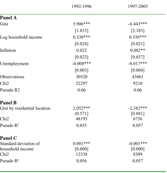
Consequently, we divide the whole sample into two sub-periods: 1992-1996 and 1997-2005. Table 2 shows the estimation results for equation (1) over the two sub-samples. In panel A we observe that when the sample is divided into two periods, the coefficient on income inequality is statistically significantly positive before 1997 (column 2) and then significantly negative after that date (column 3). If one admits the interpretation of the coefficient on the Gini index as the causal effect of income inequality on satisfaction, as do Alesina et al. (2004), then table 2 suggests that the perception of inequality changes around the year 1997: after that date

individuals are less inclined to consider themselves satisfied with reforms and, more generally with the economic situation of their country, when inequality is high, even after controlling for individual income, a number of personal characteristics, inflation and unemployment, year and region. But before that date, inequality interpreted as a measure of higher opportunities, is positively correlated with subjective evaluation of reforms. More specifically, before the break, a one percentage point increase in the Gini index leads to a 0.9 percentage point decrease in the probability of considering the country economic situation as bad; after the break the same increase in the Gini index leads to a one percentage point increase in the probability of such answer.

In panel B and C we verify that the results are robust to the use of alternative measures of inequality. One could argue that people have more local views of the income distribution and that the Gini coefficient calculated at the country level is a less precise measure of the level of inequality that the one people perceive in their closer environment. Thus, in panel B we report results based on a measure of income inequality calculated for different residential locations: large cities (over 100 000 inhabitants), smaller cities and rural areas. In panel C we measure income inequality based on our data as the standard deviation of log household income for each cross section. The results in panel B and C confirm the pattern observed in panel A: inequality measures are positively associated with the satisfaction variable in the first period, and turn out to be significantly negative in the second period.

We must emphasize that we are not trying to test whether the setback in attitudes is due to an external exogenous shock. Rather, the implicit model that we have in mind is a cumulative process of disappointment, which at a certain point goes beyond a critical threshold (exhaustion of patience). Quoting Hirschman and Rothschild (1973, p. 552): “The turning point in attitudes is

not caused by a sudden shock. It comes about “purely as a result of the passage of time – no particular outward event sets off this dramatic turnaround”. [In] “the easy early stage […] everybody seems to be enjoying the very process that will later be vehemently denounced and damned as one consisting essentially in “the rich becoming richer”. However, if we wanted to

indicate some specific events that could have contributed to the turning point in the relationship between income inequality and country satisfaction, we could refer to the fact that 1997 coincides

with the announcement by the newly-appointed government of a wave of second-generation welfare-state reforms (concerning health, pensions and education), which was met with some reluctance by the population. It is likely that this has contributed to the “reform fatigue” of the population, by reinforcing the perception of the costs imposed by reforms.

Who is most affected by inequality?

Different segments of the population may differ in their perception of income inequality. In this section, we investigate attitudes of which particular groups drive the average result (established above). First, as income inequality is initially interpreted in terms of increased opportunities, the effects should be more pronounced for those individuals who had a longer experience of the socialist regime and who have experienced the transition process from the start. Thus, we expect older people to have higher expectations at the beginning of the transition and to be more disappointed afterwards. Table 3 reports the results separately for the sample of two cohorts, i.e. those who were born before 1970 and, therefore, were at least 23 years old in 1992 and those who were born in 1970 or after. It shows that it is older people who are initially more likely to see income differentiation in terms of opportunities. Indeed, the coefficient on the Gini index is statistically significantly positive (column 1) in the regression on the sub-sample of older people, whereas it is not significant in the regression on the sub-sample of younger people (column 3). In the second period, however, the coefficient on the Gini index is negative and statistically significant for both groups. The initial positive attitude of older people towards income inequality has vanished, leaving place to a general aversion for inequality.

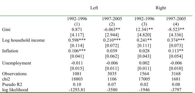
Second, we expect to see a difference in the perception of inequality depending on the ideological self-identification of individuals. Alesina et al. (2004) observed that left-wing Europeans were more affected by income inequality, as compared to right-wingers. The notions of left and right are not completely clear in the countries having experienced communism for 45 years, but we rely on the self-definition of individuals who answered the following question: “Please, describe your political opinions using the scale from 1 (left) to 7 (right).” We classified as left-wingers the respondents who replied ‘1’ and as right-wingers those who chose ‘7’ (left and right represents each about 5 percent before the break and 10 % after the break). Table 4 shows that in Poland, the

initial positive association between income inequality and satisfaction is statistically significant for right-wingers (who probably see income differentiation as a source of incentives and efficiency), but not for left-wingers (who are less likely to share this view. After 1996, a statistically significant negative association between income inequality and country satisfaction is observed in both groups.

Overall, these results suggest that the initial perception of income differentiation was more positive in groups which had longer experience of socialism or defined themselves as right-wingers. This evidence is consistent with the hypothesis that initially income differentiation in transition was taken as a sign of opportunity and efficiency, as these two groups of the population were more likely to welcome the reform at the onset of transition.

Possible alternative explanations

Due to the limitation of the data, we are unable to establish the direction of causality in the relationship between income inequality and country satisfaction. However, our objective is to assess the association between income inequality and satisfaction and to establish the existence of a break in this relationship over time. Hence, we need to rule out alternative potential explanations of the evolution in country satisfaction. The first natural suspect is time trend itself. As income inequality is rising along the whole considered period, the coefficient on the Gini index could be hiding the pure effect of time. This could happen if, the level of inequality notwithstanding, with the passage of time, people who initially had high expectations become disappointed. The inclusion of year dummies partly takes care of this issue. Alternatively, we have included a time trend in the estimation of equation (1). The results concerning the changing impact of income inequality were not altered (the coefficient on the Gini index was 5.569 (with standard deviation of 2.100) in the first period, and -13.725 (with standard deviation of 4.342) in the second period).

Second, we considered the possibility that the results are driven by seasonal variations of country satisfaction. Table 5 shows that including monthly dummies in the basic regression does not affect the results.

Third, the changing tolerance for inequality could be due to the reduced importance of the welfare state. The public attitude towards inequality certainly depends on the extent of redistribution and social protection. Keane and Prasad (2002), following Garner and Terrel (1998), argued that in Poland at the beginning of transition substantial social transfers compensated for increasing wage inequality. The mechanisms of social transfers were thus critical in ensuring political support for reform. Their period of observation stops in 1997, but official statistics show that the share of social expenditure in GDP has remained stable at around 23% since 1997. Hence, the changing tolerance for inequality does not seem to be associated with the withering away of the welfare state.

Finally, we asked whether a similar break is observable in the relationship between country satisfaction and other macroeconomic variables. We, thus, carried the same test for the presence of a structural break in the relationships between (1) unemployment rate and country satisfaction and (2) inflation rate and country satisfaction. We find that the coefficients on unemployment remain negative in all sub-periods defined by consecutive breaks, whereas the coefficients on inflation remained statistically insignificant in almost all periods. Therefore, we conclude that our main result is not driven by a change in public opinion regarding other major macroeconomic indicators.

To sum up, our results prove to be immune to several potential alternative explanations.

Other indicators of satisfaction

In order to complete the picture and provide more evidence on personal satisfaction during the transition process, we now turn to the relationship between two other subjective variables and income inequality over time. As shown in Figure 1, private satisfaction and private expectations follow a similar pattern as country satisfaction, but of smaller amplitude. Although more flat than for country satisfaction, these curves present the same downward inflexion at some point around the mid-1990’s. In addition, we observe a slight upturn around 2001 at the time when inequality receded. The level of private satisfaction and expectations is always higher than the level of country satisfaction. Interestingly, all curves share a common feature that the level of satisfaction

and expectations is higher in 2005 than it was initially in 1992.

We first check whether the estimate of private satisfaction yields results that are consistent with those in the literature with respect to the usual individual level correlates of well-being (see for example Di Tella et al., 2003). As expected, we find a U-shaped relationship between age and satisfaction, and a positive correlation with income, education, and higher occupations. Men are happier than women, a frequent observation in Central and Eastern Europe and in Latin America (Graham and Pettinato, 2002; Guriev and Zhuravskaya, 2009; Easterlin, 2008). People who live in rural areas are more satisfied and optimistic about their future standard of living than are inhabitants of urban agglomerations, who, in turn, are more satisfied than those who live in large cities. By contrast, individuals who live in rural areas view the situation of the country in a more pessimistic way.

Concerning the impact of inequality, following Hirschman’s scenario, we expect that rising inequality will end up deterring not only individuals’ appreciation of the country’s situation, but also their satisfaction with their own situation, as well as their expectations concerning their private situation.

Columns 3 and 4 of Table 6 show individuals’ expectations regarding their living conditions. Our measure of inequality is associated with higher expectations up to 1997, but it remains uncorrelated with it thereafter. This suggests that inequality is initially interpreted as an opening of new opportunities, but in the later stages of transition loses this significance in the eyes of the population. Concerning private satisfaction, columns 1 and 2 show that it is initially weakly correlated with inequality. In the second period, however, the coefficient on the Gini index becomes statistically significant and negative. We conclude that the interpretation of income inequality has changed over the period under consideration, with a visible turning point in 1997. This changing pattern of private satisfaction, in association with the rise in income inequality, may constitute an element of the famous Easterlin puzzle, i.e. the flatness of the average happiness score in developed countries, in spite of sustained GDP growth after the Second World War (Easterlin 2001). This empirical finding has stimulated an important subjective happiness

literature (see Clark et al., 2008), although it is still disputed (Stevenson and Wolfers, 2008). Two main potential explanations have been proposed: adaptation effects and comparison effects. Other attempts to explain the Easterlin paradox consist in looking for omitted variables in the estimation of the relationship between income and subjective well-being (Di Tella and MacCulloch, 2008). The findings of this paper suggest that income distribution may constitute one of these missing variables that weaken the welfare effect of growth.

Direct evidence from opinion polls

In order to find some direct evidence that the attitude towards income inequality is changing over time, we finally use several public opinion polls ran by the Public Opinion Research Center survey (CBOS, 2003). Figure 2 illustrates the weakening tolerance for income inequality, especially after 1997. Egalitarian attitudes gain in popularity, as attested by the rising percentage of people who consider that “the government should reduce differences between high and low wages” and that “inequalities of income are too large in Poland”. By contrast, the percentage of people who consider that “energetic entrepreneurs should be remunerated well in order to ensure the growth of the Polish economy”, that “future well-being in Poland requires remunerating well those who work hard”, or that “economic inequalities are necessary for economic progress”, have significantly decreased. The same pattern is visible in the data from the New Europe Barometer surveys.4 These data show that, in Poland, the proportion of individuals who declare that “incomes should be made equal so that there is no great difference in income” rather than “individual achievement should determine how much people are paid; the more successful should be paid more” rose from 24% in 1992 to 32% in 1998, and 54% in 2004.

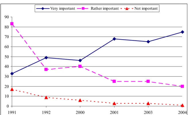
Figure 3, we use another survey (CBOS, 2004) to illustrate the share of population who consider corruption as an important problem. This sentiment increased sharply, from 32 percent in 1991 to 75 percent in 2004. Overall, it appears that the perception of the Polish population concerning fairness and efficiency of the distribution of income, deteriorated during the period under observation, with a visible turning point around 1997.

4 _{New Europe Barometer Surveys, Centre for the Study of Public Policy, University of Aberdeen.} http://www.abdn.ac.uk/cspp/nebo.shtml

These results suggest that the parallel processes of income growth and inequality were initially well accepted by Poles, who might have seen them as a promise of future shared gains. However, by the late mid-1990s, high expectations seem to have given way to more negative attitudes, fed by the rising intolerance for income inequality, the continued growth in GDP notwithstanding.

5. Conclusion

This paper provides evidence of a change in relationship between income inequality and individuals’ views of the economic situation of the country, which can partly be interpreted as a measure of support for reforms. The results suggest that income inequality was initially perceived as a positive signal of increased opportunities. However, after several years of rapid economic transformation, unfulfilled expectations and diminishing patience brought about a change in attitudes and growing inequality started to undermine satisfaction. Individuals seem to have become disappointed with transformation and skeptical about the legitimacy of the enrichment of reform winners. Various public opinion surveys confirm the changing popular opinions about the degree of corruption in the country and the desirability of high pay-offs in certain professions. Hence, the turning point in the tolerance for income inequality seems to come with the increasingly wide perception that the process that generates income distribution is itself unfair.

The findings of this paper constitute a link between the literature on subjective well-being and the political economy literature focusing on inequality and growth. It provides evidence in support of a hypothesis put forth by Acemoglu and Robinson (2000, 2002) and Perotti (1996) that growth, which is accompanied by inequality, generates dissatisfaction and, as such, carries the menace of social instability.

The results obtained in this paper offer a number of lessons for developing and transition countries: if it is important for governments to rapidly exploit the initial “window of opportunity” for reforms, it is also crucial that they adopt redistributive policies early on in the process, in order to ensure durable popular support for reforms. But the lesson can be extended to developed countries, as it stresses the importance to ensure that the functioning of the market and the process of income distribution are perceived as fair and transparent.

References

Acemoglu, D. and Robinson, J. A., 2000. ‘Why did the West extend the franchise? Democracy, inequality, and growth in historical perspective’, The Quarterly Journal of Economics 115(4), 1167-119.

Acemoglu, D. and Robinson, J. A., 2002. ‘The political economy of the Kuznets curve’, Review of Development Economics 6(2), 183-203.

Alesina, A. and Fuchs-Schuendeln, N., 2007. ‘Good Bye Lenin (or not?) – The effect of communism on people’s preferences,’ American Economic Review 97, 1507-1528.

Alesina, A. and Angeletos, G-M., 2005. ‘Fairness and redistribution: US versus Europe’, American Economic Review 95, 913-35.

Alesina, A. and la Ferrara, E., 2005. ‘Preferences for redistribution in the land of opportunities’, Journal of Public Economics 89, 897-931.

Alesina, A., Di Tella, R. and MacCulloch, R., 2004. ‘Inequality and happiness: Are Europeans and Americans different?’, Journal of Public Economics 88, 2009–2042.

Alesina, A. and Perotti, R., 1996. ‘Income distribution, political instability, and investment’, European Economic Review 40(6), 1203-1228.

Alesina, A. and Rodrik, D., 1994. ‘Distributive politics and economic growth’, The Quarterly Journal of Economics 109(2), 465-90.

Andrews, D.W.K., 1993. ‘Test for parameter instability and structural change with unknown change point’, Econometrica 61(4), 821-856.

Brainerd, E., 1998. ‘Winners and losers in Russia’s economic transition’, American Economic Review 88, 1094-1116.

CBOS, 2003. ‘Attitudes towards income inequality’, Warsaw. CBOS, 2004. ‘The perception of corruption in Poland’, Warsaw.

Clark, A., Frijters, E. P. and Shields, M., 2008. ‘Relative Income, Happiness and Utility: An Explanation for the Easterlin Paradox and Other Puzzles’, Journal of Economic Literature 46, 95-144.

Deininger, K. and Squire, L., 1996. ‘A new data set measuring income inequality’, World Bank Economic Review 10 (3), 565-591.

Denisova, I., Markus, E. and Zhuravskaya, E., 2008. ‘What Russians think about transition: Evidence from RLMS survey’, CEFIR and NES working paper n°113.

Desai, R. M. and Olofsgärd, A., 2006. ‘Political constraints and public support for market reform’. IMF Staff Papers, 53.

Di Tella, R, MacCulloch, R. and Oswald, A., 2003. ‘The macroeconomics of happiness’, Review of Economics and Statistics 85(4), 809–827.

Di Tella, R, MacCulloch, 2008. ‘Gross national happiness as an answer to the Easterlin Paradox?’, Journal of Development Economics, 86, 22-42.

Easterlin, R., 2001. ‘Income and happiness: a unified theory’, Economic Journal 111, 1-20. Easterlin, R., 2008. ‘Lost in transition; Life satisfaction on the road to capitalism’, IZA DP 3409. Ferrer-i-Carbonell, A., 2005. ‘Income and well-being: An empirical analysis of the comparison

income effect’, Journal of Public Economics 89, 997-1019.

Fong, Ch., 2001. ‘Social preferences, self-interest, and the demand for redistribution’, Journal of Public Economics 82, 225-246.

Garner, T. and Terrell, K., 1998. ‘A Gini Decomposition of inequality in the Czech and Slovak Republics during the transition’, Economics of Transition 6(1), 23-46.

Graham, C. and Pettinato, S., 2002. ‘Frustrated achievers: winners, losers, and subjective well being in new market economies’, Journal of Development Studies 38, 100–140.

Guriev, S.M. and Zhuravskaya, E.V., 2009, ‘(Un)Happiness in Transition’, forthcoming in Journal of Economic Perspectives.

Hirschman, A. and Rothschild, M., 1973. ‘The changing tolerance for income inequality in the course of economic development’, Quarterly Journal of Economics 87, 544-566.

Keane, M. and Prasad, E., 2006. ‘Inequality, transfers and growth: new evidence from the economic transition in Poland’, Review of Economics and Statistics 84(2), pp. 324-341.

Kornai, J., 2006. ‘The great transformation of Central Eastern Europe’, Economics of Transition 14(2), 207-244.

Krastev, I., 2007. ‘The strange death of the liberal consensus’, Journal of Democracy 18 (4). Milanovic, B., 1998. ‘Income, inequality, and poverty during the transition from planned to

market economy. The first comprehensive review of social effects of transition in 18 countries’. World Bank Regional and Sectoral Studies.

Perotti E., 1996, “Growth, income distribution, and democracy: what the data day”, Journal of Economic Growth, 1, 149-187.

Persson, T. and Tabellini, G., 1994. ‘Is inequality harmful for growth?’, American Economic Review 8, 600–621.

Ravallion, M. and Lokshin, M., 2000. ‘Who wants to redistribute? The tunnel effect in 1990s Russia’, Journal of Public Economics 76(1), 81-104.

Sanfey, P. and Teksoz, U., 2007. ‘Does transition make you happy?’, Economics of Transition 15(4), 707-731.

Senik C., 2004,"When information dominates comparison. Learning from Russian subjective panel data", Journal of Public Economics 88 (9-10), 2099-2133.

Senik, C., 2005, “What can we learn from subjective data ? The case of income and well-being”, Journal of Economic Surveys 19 (1), 43-63.

Senik C., 2008, "Ambition and jealousy. Income interactions in the "Old Europe" versus the "New Europe" and the United States", Economica 75, 299-.

Stevenson Betsey and Justin Wolfers, 2008, “Economic growth and subjective well-being: reassessing the Easterlin Paradox”, Brookings Papers on Economic Activity, Spring.

Fig. 1. Satisfaction variables, real GDP and the Gini coefficient, 1992-2005 (yearly averages) 1 1,5 2 2,5 3 3,5 1992 1993 1994 1995 1996 1997 1998 1999 2000 2001 2002 2003 2004 2005 0,3 0,32 0,34 0,36 0,38 0,4

Left axis Country satisfaction Left axis Private satisfaction Left axis Private expectations Left axis GDP real, 1992=1 Right axis Gini

Figure 2. Opinions concerning income inequality, Poland 1994-2003 (%) 0 10 20 30 40 50 60 70 80 90 100 1994 1997 1998 1999 2003

Energetic entrepreneurs should be remunerated well to ensure the growth of the Polish economy Large inequalities of income are necessary to guarantee future well-being

Inequalities of income are too large in Poland

Figure 3. “In your opinion, how important is the corruption problem in Poland?” (%) 0 10 20 30 40 50 60 70 80 90 1991 1992 2000 2001 2003 2004

Very important Rather important Not important

Source: CBOS (2004). Percentage of people who answer positively the following question: “In your opinion, how important is the corruption problem in Poland: very important/rather important/not very important/not important”.

Table1. Test of a break in the relationship between income inequality and country satisfaction

Wald test Gini index before the break

Gini index after the break

(1) (2) (3) 1992 1993 7.09 5.685*** [1.668] [2.056] -1.394 1994 3.98 4.418** [2.034] -1.586 [2.223] 1995 6.31 4.358*** [1.644] [2.592] -3.299 1996 18.44 5.828*** [1.732] -6.116*** [2.177] 1997 8.10 3.583* [1.891] -6.040** [2.821] 1998 7.00 3.202* [1.833] -6.155** [3.035] 1999 5.54 2.804 [1.802] -5.828* [3.203] 2000 14.12 3.312* [1.700] -8.910*** [2.810] 2001 3.42 1.231 [1.928] -7.861* [4.526] 2002 0.83 0.631 [1.869] -6.053 [7.075] 2003 1.96 0.791 [1.845] -10.747 [8.033] 2004 0.53 0.074 [1.855] 4.600 [5.943] 2005

The numbers in column (1) are values of chi2 corresponding to Wald statistics for all possible breakpoints. We test the existence of a break, trimming at 15%. The critical value from Andrews (1993) for one parameter and trimming at 15% is 8.85 at the 5% level. In columns (2) and (3) we show the coefficients of the Gini index obtained for the periods before and after each break.

Table 2. Country satisfaction and income inequality before and after the break. Ordered logit

1992-1996 1997-2005 Panel A

Gini 5.906*** -6.443***

[1.815] [2.183]

Log household income 0.330*** 0.330***

[0.024] [0.021] Inflation 0.022 0.082** [0.023] [0.037] Unemployment -0.008*** -0.017*** [0.003] [0.004] Observations 30520 43061 Chi2 52297 9210 Pseudo R2 0.06 0.06 Panel B

Gini by residential location 2.052***

(0.571] -2.382*** [0.881] Chi2 48193 6756 Pseudo R² 0.055 0.057 Panel C Standard deviation of household income 0.001*** [0.000] -0.001*** [0.000] Chi2 12338 8309 Pseudo R² 0.056 0.057

The dependent variable, country satisfaction, scores the answers to the following questions: How do you assess current economic situation in Poland? Answers from 1 “very bad” to 5 “very good” (Country satisfaction). Controls in panel A include gender, age, age-squared, education, residential location (except in panel B), labor market status, occupation, region dummies, and year dummies. In Panels B and C log household income, inflation and unemployment are also included. Gini coefficients and standard deviation of household income are calculated for each successive representative cross-section. All standard errors (in brackets) are clustered by cross-section. *, ** and *** denote significance at the 10, 5 and 1% levels respectively.

Table 3. Country satisfaction and income inequality: cohort effects. Ordered logit.

Born before 1970 Born after 1969

1992-1996 1997-2005 1992-1996 1997-2005

(1) (2) (3) (4)

Gini 6.351*** -6.386*** 1.237 -6.791***

[1.802] [2.265] [2.834] [2.410]

Log household income 0.335*** 0.365*** 0.295*** 0.232***

[0.028] [0.022] [0.065] [0.035] Regional unemployment -0.009*** -0.018*** -0.005 -0.011* [0.003] [0.004] [0.009] [0.006] Inflation rate 0.021 0.088** 0.034 0.049 [0.023] [0.040] [0.032] [0.039] Observations 27851 34818 2669 8243 chi2 644537 11502 5378140 1761 Pseudo R2 0,05 0,06 0,06 0,05 log likelihood -31910 -40627 -2955 -9488

Controls include gender, age, age-squared, education, residential location, labour market status, occupation, region dummies, and year dummies. All standard errors (in brackets) are clustered by cross-section. *, ** and *** denote significance at the 10, 5 and 1% levels respectively.

Table 4. Country satisfaction and income inequality: left and right. Ordered logit.

Left Right

1992-1996 1997-2005 1992-1996 1997-2005

(1) (2) (3) (4)

Gini 0.871 -6.063** 12.341** -8.523**

[4.117] [2.944] [4.820] [4.336]

Log household income 0.598*** 0.210*** 0.241** 0.374***

[0.114] [0.072] [0.111] [0.073] Inflation 0.106*** 0.039 0.028 0.113** [0.041] [0.062] [0.043] [0.054] Unemployment -0.011 -0.006 0.002 -0.006 [0.015] [0.011] [0.011] [0.010] Observations 1081 3035 1564 3168 chi2 18803 1106 17005 1681 Pseudo R2 0.10 0.07 0.02 0.08 log likelihood -1293.81 -3580 -1946 -3797

Controls include gender, age, age-squared, education, residential location, labour market status, occupation, region dummies, and year dummies. All standard errors (in brackets) are clustered by cross-section. *, ** and *** denote significance at the 10, 5 and 1% levels respectively.

Table 5. Country satisfaction: controlling for seasonality. Ordered logit. 1992-1996 1997-2005 Gini 6.289*** -6.061*** [2.061] [1.669] Inflation 0.085*** -0.046 [0.031] [0.047] Unemployment -0.010*** -0.017*** [0.003] [0.004] _Imonth_2 0.015 [0.117] _Imonth_3 -0.026 -0.322*** [0.103] [0.112] _Imonth_5 0.096 -0.266** [0.116] [0.105] _Imonth_6 0.187** [0.081] _Imonth_7 0.319*** -0.363*** [0.117] [0.128] _Imonth_9 0.086 -0.214* [0.089] [0.115] _Imonth_10 0.427*** [0.106] _Imonth_11 0.266** -0.217** [0.109] [0.110] _Imonth_12 0.522*** [0.121] Observations 30520 43061 chi2 20463.40 11758.02 Pseudo R2 0.06 0.06 log likelihood -34853 -50140

Controls include gender, age, age-squared, education, residential location, labour market status, occupation, region dummies, and year dummies. All standard errors (in brackets) are clustered by cross-section. *, ** and *** denote significance at the 10, 5 and 1% levels respectively.

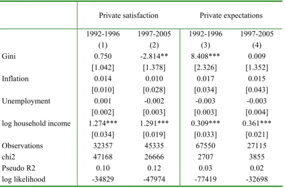
Table 6. A reversal in private expectations and satisfaction

Private satisfaction Private expectations

1992-1996 1997-2005 1992-1996 1997-2005 (1) (2) (3) (4) Gini 0.750 -2.814** 8.408*** 0.009 [1.042] [1.378] [2.326] [1.352] Inflation 0.014 0.010 0.017 0.015 [0.010] [0.028] [0.034] [0.043] Unemployment 0.001 -0.002 -0.003 -0.003 [0.002] [0.003] [0.003] [0.004]

log household income 1.274*** 1.291*** 0.309*** 0.361***

[0.034] [0.019] [0.033] [0.021]

Observations 32357 45335 67550 27115

chi2 47168 26666 2707 3855

Pseudo R2 0.10 0.12 0.03 0.02

log likelihood -34829 -47974 -77419 -32698

The dependent variables are the answers to the following questions: Do you think that in a year your life and the life of your family will be: Answers from 1 “much worse” to 5 “much better than now” (Private expectations); How do you and your family live? Answers from 1 “very bad” to 5 “very good” (Private satisfaction). Controls include gender, age, age-squared, education, residential location, labor market status, occupation, regional dummies, time trend, and year dummies. Gini coefficients are calculated for each successive representative section. All standard errors (in brackets) are clustered by cross-section. *, ** and *** denote significance at the 10, 5 and 1% levels respectively.

Appendix

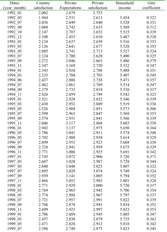
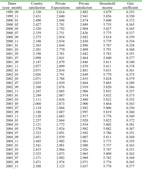
Table A1: Subjective variables, household income and the Gini coefficient: mean values of variables for each cross-section.

Dates (year_month) Country satisfaction Private Expectations Private satisfaction Household income Gini coefficient 1992_01 2.002 2.679 2.753 1992_05 1.944 2.531 2.613 5.454 0.323 1992_07 2.036 2.849 2.640 5.528 0.331 1992_09 2.060 2.742 2.635 5.569 0.312 1992_10 2.147 2.707 2.652 5.515 0.339 1992_12 2.108 2.453 2.610 5.467 0.320 1993_01 2.124 2.637 2.659 5.516 0.353 1993_03 2.126 2.641 2.677 5.528 0.355 1993_05 2.085 2.741 2.713 5.527 0.324 1993_07 2.124 2.700 2.628 5.490 0.325 1993_09 2.272 3.046 2.663 5.486 0.379 1993_11 2.347 3.169 2.720 5.532 0.347 1994_01 2.343 2.924 2.788 5.488 0.351 1994_03 2.235 2.704 2.703 5.407 0.345 1994_06 2.437 2.886 2.738 5.471 0.357 1994_07 2.462 2.861 2.769 5.514 0.347 1994_09 2.379 2.733 2.818 5.510 0.337 1994_11 2.426 2.859 2.749 5.542 0.323 1995_01 2.521 2.928 2.832 5.546 0.339 1995_03 2.430 2.952 2.809 5.519 0.336 1995_05 2.526 2.904 2.851 5.573 0.306 1995_07 2.599 2.963 2.847 5.569 0.353 1995_09 2.574 2.931 2.841 5.566 0.339 1995_11 2.606 3.117 2.868 5.683 0.358 1996_01 2.943 3.137 2.975 5.650 0.364 1996_03 2.786 3.041 2.911 5.574 0.348 1996_05 2.702 2.988 2.938 5.614 0.329 1996_07 2.699 2.953 2.923 5.668 0.336 1996_09 2.724 2.941 2.959 5.675 0.329 1996_11 2.771 3.006 2.925 5.691 0.342 1997_01 2.745 3.072 2.906 5.726 0.371 1997_03 2.687 3.028 2.987 5.728 0.344 1997_05 2.840 3.048 3.023 5.807 0.332 1997_07 2.895 3.029 3.074 5.749 0.324 1997_09 2.939 3.141 3.005 5.794 0.352 1997_11 2.866 3.052 2.985 5.801 0.328 1998_01 2.771 2.929 3.000 5.720 0.337 1998_03 2.769 2.965 2.942 5.706 0.354 1998_05 2.774 2.988 2.967 5.797 0.337 1998_07 2.721 2.957 2.991 5.822 0.339 1998_09 2.746 2.878 2.943 5.834 0.352 1998_11 2.699 2.923 2.997 5.823 0.353 1999_01 2.706 2.889 2.945 5.805 0.347 1999_03 2.457 2.830 2.879 5.735 0.363 1999_05 2.471 2.828 2.912 5.818 0.342 1999_07 2.396 2.749 2.875 5.823 0.345

Table A1 continued. Dates (year_month) Country satisfaction Private Expectations Private satisfaction Household income Gini coefficient 1999_09 2.330 2.814 2.882 5.879 0.353 1999_11 2.431 2.840 2.941 5.856 0.350 2000_01 2.490 2.848 2.874 5.800 0.372 2000_02 2.427 2.781 2.889 5.755 0.365 2000_05 2.320 2.792 2.904 5.827 0.365 2000_07 2.339 2.751 2.826 5.775 0.337 2000_09 2.375 2.854 2.882 5.814 0.359 2000_11 2.348 2.834 2.830 5.779 0.354 2001_01 2.383 2.844 2.896 5.787 0.328 2001_03 2.201 2.770 2.809 5.791 0.368 2001_05 2.198 2.781 2.842 5.783 0.351 2001_07 2.098 2.841 2.864 5.840 0.377 2001_09 2.147 2.879 2.846 5.811 0.340 2001_11 2.077 2.899 2.870 5.811 0.378 2002_01 2.071 2.834 2.881 5.831 0.361 2002_03 2.056 2.791 2.849 5.779 0.375 2002_05 2.071 2.788 2.835 5.824 0.379 2002_07 2.035 2.839 2.864 5.885 0.389 2002_09 2.160 2.876 2.910 5.820 0.366 2002_11 2.247 2.885 2.906 5.852 0.357 2003_01 2.249 2.867 2.914 5.832 0.373 2003_03 2.111 2.836 2.880 5.822 0.355 2003_05 2.060 2.873 2.900 5.864 0.363 2003_07 2.134 2.804 2.882 5.806 0.356 2003_09 2.188 2.887 2.997 5.819 0.360 2003_11 2.120 2.683 2.917 5.778 0.369 2004_01 2.257 2.864 2.920 5.822 0.372 2004_03 2.121 2.772 2.934 5.802 0.381 2004_05 2.370 2.924 2.982 5.882 0.367 2004_07 2.323 2.891 2.942 5.786 0.351 2004_09 2.451 2.939 3.007 5.811 0.369 2004_11 2.445 2.902 2.961 5.773 0.355 2005_01 2.541 2.981 2.980 5.737 0.363 2005_03 2.415 2.966 2.926 5.747 0.351 2005_05 2.525 3.073 2.965 5.809 0.362 2005_07 2.371 2.903 2.989 5.782 0.369 2005_09 2.471 2.974 2.971 5.776 0.365 2005_11 2.588 3.123 3.037 5.778 0.377

Country satisfaction: How do you assess current economic situation in Poland? Answers from 1 “very bad” to 5 “very good”; Private expectations: Do you think that in a year your life and the life of your family will be: Answers from 1”much worse” to 5”much better” than now; Private satisfaction: How do you and your family live? Answers from 1 “very bad” to 5 “very good”. Household income is the logarithm of net total monthly household income per capita, deflated by the monthly CPI. Gini coefficients are calculated for each successive representative cross-section.

Table A2. The socio-demographic structure of the sample, yearly averages.

Panel A

Year Female Age Secondary

education

Rural areas Urban areas Large cities

1992 0.55 46.77 0.34 0.42 0.52 0.28 1993 0.55 47.93 0.35 0.42 0.52 0.28 1994 0.48 47.89 0.37 0.40 0.53 0.28 1995 0.55 48.24 0.37 0.40 0.51 0.29 1996 0.55 47.61 0.39 0.37 0.55 0.28 1997 0.57 47.53 0.41 0.37 0.52 0.31 1998 0.56 47.74 0.41 0.37 0.53 0.30 1999 0.56 48.17 0.43 0.37 0.52 0.30 2000 0.55 48.13 0.45 0.37 0.50 0.32 2001 0.56 47.86 0.44 0.36 0.49 0.32 2002 0.55 48.46 0.46 0.35 0.46 0.35 2003 0.55 47.82 0.46 0.37 0.47 0.33 2004 0.52 46.89 0.46 0.41 0.51 0.29 2005 0.53 46.73 0.44 0.37 0.51 0.30

Urban areas are defined as having no more than 100 000 inhabitants. Large cities are defined as having over 100 000 inhabitants.

Panel B

Year Unemployed Pensioners Farm Not working Unqualified workers Qualified workers Higher occupations Self-employed 1992 0.08 0.34 0.11 0.07 0.06 0.14 0.06 0.03 1993 0.05 0.44 0.09 0.03 0.04 0.10 0.06 0.04 1994 0.04 0.45 0.09 0.02 0.04 0.10 0.06 0.04 1995 0.06 0.43 0.08 0.04 0.04 0.10 0.06 0.04 1996 0.08 0.37 0.07 0.06 0.04 0.10 0.07 0.04 1997 0.08 0.35 0.06 0.06 0.04 0.10 0.08 0.04 1998 0.07 0.37 0.06 0.05 0.04 0.09 0.07 0.04 1999 0.08 0.37 0.06 0.05 0.04 0.09 0.07 0.04 2000 0.09 0.37 0.06 0.05 0.03 0.08 0.07 0.04 2001 0.12 0.37 0.05 0.05 0.03 0.08 0.06 0.04 2002 0.13 0.37 0.05 0.04 0.03 0.07 0.07 0.04 2003 0.12 0.35 0.05 0.05 0.03 0.07 0.07 0.04 2004 0.12 0.34 0.06 0.05 0.03 0.07 0.07 0.04 2005 0.11 0.33 0.05 0.05 0.04 0.08 0.05 0.03

Higher occupations include directors, presidents and managerial staff in public administration, liberal professions with higher education, engineers, school directors, physicians, and lawyers.

Table A3. Macroeconomic variables: yearly averages

Year Nominal GDP Real GDP

growth Unemployment rate Gini coefficient (our data) Gini coefficient UNICEF data 1992 114243 102.6 13.1 0.325 0.274 1993 155780 103.8 14.9 0.348 0.317 1994 210377 105.2 16.5 0.343 0.323 1995 306318 107.0 15.2 0.339 0.321 1996 385448 106.2 14.4 0.342 0.328 1997 469372 107.1 11.6 0.342 0.334 1998 549467 105.0 10.0 0.345 0.326 1999 665688 104.5 11.9 0.350 0.334 2000 744378 104.3 13.9 0.359 0.345 2001 779564 101.2 16.1 0.356 0.341 2002 808578 101.4 17.7 0.371 0.353 2003 843156 103.9 18.0 0.363 0.356 2004 924538 105.3 19.6 0.366 - 2005 982565 103.6 18.2 0.353 -

Source: Polish Central Statistical Office (GUS). Gini coefficients calculated using yearly average household income in our data. The estimates of the Gini coefficient from the UNICEF Database (IRC TransMONEE 2005) are based on interpolated distributions from grouped data from household budget surveys reported to the MONEE project.

Table A4. Country satisfaction, ordered logit. (1) (2) Gender -0.061*** -0.062*** [0.021] [0.021] Age -0.031*** -0.032*** [0.003] [0.003] Age squared 0.000*** 0.000*** [0.000] [0.000]

Log household income 0.334*** 0.329***

[0.016] [0.016] Education 0.117*** 0.115*** [0.024] [0.024] Unemployed -0.032 -0.030 [0.028] [0.027] Pensioners -0.110*** -0.107*** [0.023] [0.023] Farm -0.173*** -0.170*** [0.034] [0.034] Unqworkers -0.086** -0.086*** [0.034] [0.033] Qualified workers -0.019 -0.021 [0.031] [0.031] Not working 0.133*** 0.129*** [0.039] [0.038] Higher occupations 0.189*** 0.189*** [0.038] [0.038] Self-employed 0.040 0.039 [0.047] [0.047] Students 0.211*** 0.209*** [0.041] [0.041] Rural areas -0.152*** -0.154*** [0.022] [0.023] Large cities -0.022 -0.037 [0.025] [0.025] West -0.076** -0.087*** [0.031] [0.031] Centre West -0.017 -0.064** [0.030] [0.031] Centre -0.132*** -0.202*** [0.029] [0.030] East -0.204*** -0.247*** [0.039] [0.039] South-East -0.083*** -0.150*** [0.030] [0.032] South-West 0.149*** 0.058* [0.031] [0.034]

Table A4, continued cut1:Constant -0.405 2.616 [0.614] [2.450] cut2:Constant 2.066*** 5.088** [0.612] [2.449] cut3:Constant 4.077*** 7.101*** [0.614] [2.449] cut4:Constant 8.618*** 11.643*** [0.625] [2.467] Gini 0.074 0.087 [1.865] [1.834] Unemployment -0.012*** [0.002] Inflation 0.032 [0.023] Observations 73581 73581 chi2 4633.67 4531.66 Pseudo R2 0.05 0.05 log likelihood -85275.60 -85242.27

Country satisfaction answers the following question: How do you assess current economic situation in Poland? Answers from 1 “very bad” to 5 “very good”; Gini coefficients are calculated for each successive representative cross-section. Yearly dummies included. Omitted variables: men, less than secondary education, urban areas (with less than 100 000 inhabitants), employees, and north region. All standard errors (in brackets) are clustered by cross-section.* significant at 10%, ** significant at 5%, *** significant at 1%.