TENSOR OBJECT CLASSIFICATION VIA MULTILINEAR DISCRIMINANT ANALYSIS NETWORK

HAL Id: hal-01380110

https://hal-univ-rennes1.archives-ouvertes.fr/hal-01380110

Submitted on 24 Feb 2017

HAL is a multi-disciplinary open access

archive for the deposit and dissemination of

sci-entific research documents, whether they are

pub-lished or not. The documents may come from

teaching and research institutions in France or

abroad, or from public or private research centers.

L’archive ouverte pluridisciplinaire HAL, est

destinée au dépôt et à la diffusion de documents

scientifiques de niveau recherche, publiés ou non,

émanant des établissements d’enseignement et de

recherche français ou étrangers, des laboratoires

publics ou privés.

TENSOR OBJECT CLASSIFICATION VIA

MULTILINEAR DISCRIMINANT ANALYSIS

NETWORK

Rui Zeng, Jiasong Wu, Lotfi Senhadji, Huazhong Shu

To cite this version:

Rui Zeng, Jiasong Wu, Lotfi Senhadji, Huazhong Shu. TENSOR OBJECT CLASSIFICATION VIA

MULTILINEAR DISCRIMINANT ANALYSIS NETWORK. 40th IEEE International Conference on

Acoustics, Speech, and Signal Processing (ICASSP), Apr 2014, Brisbane, Australia. pp.1971–1975.

�hal-01380110�

TENSOR OBJECT CLASSIFICATION VIA MULTILINEAR DISCRIMINANT ANALYSIS

NETWORK

Rui ZengH, Jiasong Wu*t+-, Lotfi Senhadjitt- and Huazhong ShuH

*

LIST, Key Laboratory of Computer Network and Information Integration (Southeast University), Ministry of Education, N anjing 210096, China

t

INSERM U 1099,35000 Rennes, France

t

Laboratoire Traitement du Signal et de l'Image, Universit de Rennes 1, Rennes, France - Centre de Recherche en Information Biomedicale Sino-fran�ais (CRIDs)

E-mail: zengrui@seu.edu.cn.jswu@seu.edu.cn.lotfi.senhadji@univ-rennesI.fr.shu.list@seu.edu.cn

ABSTRACT

This paper proposes an multilinear discriminant analysis net­ work (MLDANet) for the recognition of multidimensional objects, knows as tensor objects. The MLDANet is a variation of linear discriminant analysis network (LDANet) and prin­ cipal component analysis network (PCANet), both of which are the recently proposed deep learning algorithms. The ML­ DANet consists of three parts: 1) The encoder learned by MLDA from tensor data. 2) Features maps obtained from de­

coder. 3) The use of binary hashing and histogram for feature pooling. A learning algorithm for MLDANet is described. Evaluations on UCFll database indicate that the proposed MLDANet outperforms the PCANet, LDANet, MPCA+LDA,

and MLDA in terms of classification for tensor objects. Index Terms- Deep learning, MLDANet, PCANet, L­ DANet, tensor object classification

1. INTRODUCTION

One key ingredient for the success of deep learning in visual content classification is the utilization of convolution archi­ tectures [1,2,3], which are inspired by the structure of human visual system [4]. A convolution neural network (CNN) [2] consists of multiple trainable stages stacked on the top of each other, following a supervised classifier. Each stage of CNN is organized in two layers: convolution layer and pooling layer.

Recently, Chan et al. [5] proposed a new convolutional ar­ chitecture, namely, principal component analysis network (P­ CANet), which uses the most basic operation (PCA) to learn

This work was supported by the National Basic Research Program of China under Grant 201lCB707904, by the NSFC under Grants 61201344, 61271312, 11301074, by the SRFDP under Grants 20110092110023 and 20120092120036, the Project-ponsored by SRF for ROCS, SEM, by Nat­ ural Science Foundation of Jiangsu Province under Grant BK2012329 and by Qing Lan Project. This work is supported by INSERM postdoctoral fel­ lowship.

the dictionary in the convolution layer and the pooling lay­ er is composed of the simplest binary hashing and histogram. The PCANet leads to some pleasant and thought-provoking surprises: such a basic network has achieved the state-of-the­ art performance in many visual content datasets. Meanwhile, Chan et al. [5] proposed linear discriminant analysis network (LDANet) as a variation of PCANet.

However, PCANet and LDANet are deteriorated when dealing with visual content, which is naturally represent­ ed as tensor objects. That is because when using PCANet or LDANet, the multidimensional patches, taken from visual content, are simply converted to vector to learn the dictionary. It is well known that vector representation of patches breaks the natural structure and correlation in the original visual content. Moreover, it may also, suffers from the so-called curse of dimensionality [6].

Recently, there is growing interest in the tensorial exten­ sion of deep learning algorithms. Yu et al. [7] proposed deep tensor neural network, which can be seen as a tensorial ex­ tension of deep neural network (DNN), outperforms DNN in large vocabulary speech recognition. Hutchinson et al. [8] p­ resented the tensorial extension of deep stack neural network, which has been successfully used in MNIST handwriting im­ age recognition, phone classification, etc. However, the simi­ lar tensorial extension research has not been reported for deep learning algorithms with convolutional architecture.

In this paper, we propose a simple deep learning algorith­ m for tensor object classification, that is, multilinear discrim­ inant analysis network, which is a tensorial extension of P­ CANet and LDANet. The simulation on UCF 11 database [9] demonstrates that the MLDANet outperforms PCANet and L­ DANet in terms of classification accuracy for tensor objects.

2. REVIEW OF MLDA

In this section, we briefly review MLDA [10], which is a mul­ tilinear extension of LDA. The MLDA obtains discriminative

Fig. !. The process of elementary multilinear projection (EM­ P).

Fig. 2. Tensor-to-vector projection (TVP).

features through maximizing the Fisher's discrimination cri­ terion, which is described as follows.

An Nth tensor object is denoted as

X E

R/l X I2 X ... X IN.

It is addressed by N indices

in,

n

=

1,2, . . . ,N, and each

in

addresses the n-mode of

X.

The n-mode tensor product of

X

by a matrix U

E

nJ"xI" is defined as:

(Xx."U)(i" .. ,i"_l,j,,,i,,+l, .. ,iN)=

L

X(i1, . . ,iN rU(j,,,i,,)·

(1) The projection from tensor

X E

nItxI2x···xIN to a s­ calar

Y

can be described as follows:

(2) where

{u(n)T }t:=1

is a set of unit projection vectors. This ten­ sor to scalar projection is called elementary multilinear pro­ jection (EMP), which consists of one projection vector in each mode. An EMP of a tensor

X E

R/,XI2XI3 is illustrated in Fig. 1.

The tensor-to-vector projection (TVP) from a tensor

X E

nItxI2x ... xIN to a vector

Y

E

RP is to find a vector set

{u�n)1',

n

=

1,

... , N}:=l'

which are able to do P times EM­

P. The process can be described as:

- X

N {(n)1' -

_N

_}

_P

Y -

Xn=l up

,n - 1,

... , p=l,

(3)

whose pth component is obtained from the pth EMP as y

(p)

=

(l)T

(2)T

(N)T .

.

X

X 1 up X 2 Up ... X N Up

• Flg. 2 shows the schematlc

plot for TVP.

Suppose that we are given

M

input tensor objects,

{Xm}�=l

E

R/IX ... xIN, which contains C classes. The pth projected scalar of

{Xm}�=l

are defined as

{

y

mp}�=l'

where

Ymp

= Xm

Xt:=l {u�n)T }t:=1'

So the between-class s­ catter matrix and the within-class scatter matrix for pth scalar

Fig. 3. The architecture of two-stage MLDANet. tensor objects are defined as follows, respectively:

C M

Skp

=

L Nc(ycp _yp)2, SWp

=

L (Ymp _Ycmp)2,

(4)

c=l

m=l

where

YP

=

(ljM)LmYmp' YCp

=

(ljNc)LmEcYmp'

C

is the number of classes,

Nc

is the number of tensor objects in class c, and

Cm

is the class label for the mth tensor objec­

t. Thus, the Fishers Discriminant criterion for the pth scalar tensor objects is

FpY

=

Sk j Sw

p

p

. The objective of MLDA is to determine a set of P EMP s

{u�n)1',

n

=

1,

... , N}:=l

satisfying the following conditions:

)1'

{ u�n

,n

=

1,

... , N}

=

arg max

F;

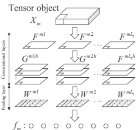
(5) 3. THE ARCHITECTURE OF MLDANET

Fig. 3 shows the architecture of MLDANet for third-order tensor objects classification. It contains two convolutional layers and one pooling layer. The filter bank in each convolu­ tional layer is learned independently. We use binary hashing and histogram as pooling operation for the features extracted from the first two convolutional layers.

3. 1. The first stage of MLDANet

For the given

M

third-order tensor objects

{Xm}�=l

E

R/l X It X I3, which contains

C

classes, we take tensor patch­ es around the I-mode and 2-mode by taking all 3-mode elements of mth tensor object, i.e., the tensor patch size is

k1

x

k2 X

13, we collect all (overlapping) It x

12

ten­

sor patches from

X

m

. The tensor patches have the same class with

X

m

. We put these tensor patches into a set

tm = {tm,q E

n

k,

x k2 X Is

}

���

I2. By repeating the above process for every tensor objects, we can get all tensor patches

t

=

{tm}�=l

for learning filter bank in the first stage. Let

L1

be the number of filters in the first stage. We apply

1

L

{(I) (2)

(3)

}Ll

MLDA to

t

to earn the

1

vector sets

up , up , up p=l'

Each tensor patch is converted into Ll scalars by using

{U(l) U(2) U(3)}L,

_{p , p}

_,

_{P p}

_=l·

Thus the lth feature map of tensor , object

Xm

in the first stage is defined as:

Fml =

mat(t

m,q n-1

x3

_

{u(n)T})

_I

E nJ,xI2

_,

q

=

1, . . . ,h X

12,

(6) where mat( v

)

is a function that maps v

E n 1, h

on a matrix

F E nJ,xI2.

For each tensor object, we can obtain

L1

feature map­ s of size h

x 12.

We denote these feature maps of mth tensor object in the first stage with

{Fml

E nJ,xI2,1

=

1,

... , L1};;;= 1.

The feature maps of each tensor object cap­ ture the main variation of original data.

3.2. The second stage of MLDANet

Through the first stage, the tensor object is already mapped into low-dimensional tensor feature, the dimension of the 3-mode is much lower than that of the I-3-mode and 2-3-mode. That is to say, the redundancy of 3-mode has been greatly reduced. Therefore, for the simplicity of computation and the conve­ nience of building network, we use the conventional LDA in the second stage to learn the filter bank. The number of filters in the second stage is

L2.

Around each pixel, we take a

k1 x k2

patch, and col­ lect all (overlapping) patches of all the feature maps

_.

Fml,

{

}J,Xh

nk,xk2

_{h h d}

t th I.e.,

rml,q q=l

E

l'v w ere eac

rml,q

eno es e

qth vectorized patch in the lth feature map of mth tensor ob­ ject. We then subtract the patch mean from each patch, and construct the matrix

Rml = [rml,l, rml,2,· .. , rml,I,

XI2]

for them, where

Rml

belongs to the same class with the mth ten­ sor object. Let

Se

is the set of matrix

Rml

in class c. We

then compute the class mean

f e

and the mean of class

f

as follows:

So, the within-class scatter matrix and the between-class scatter matrix are defined respectively as follows:

c

Sw

2:) L

(Rml - fe)(Rml - fe)T

I

ISel),

(8)

e=l mlESc

C

L(fe - r)(fe - ff

IC.

e=l

(9)

We then get w*

E nk,k2XL2

by maximizing the Fisher's

discriminant criterion as follows:

* Tr

(

w

TS

B w

)

w

= arg

max

(T S

)

' s.t. wT w

=

h2•

(10) w Tr w WW

By using mat function, each column of w* is converted into

matrix

{v

h E n k, x k2

}

t�

1.

These matrices are treated as the

filter bank in the second stage. Let the hth output of the lth feature map for the mth tensor object in the second stage be

Cm1h = Rml

*

vh,h =

1,

... ,L2,1 =

1,

... ,L1,

(11)

where * denotes 2D convolution [2], and the boundary of

Rml

is zero-padded before convolving with

Vh

so as to make

Cm1h

have the same size as

Rml.

The number of output feature maps of the second stage is

L1L2.

One or more additional stages can be built if a deep architecture is found to be bene­ ficial.

3.3. The pooling layer in MLDANet

First, we binarize each feature map by using Heaviside step function H

(

.

)

, whose value is one for positive entries and zero otherwise. The binarized feature maps are denoted by

Cm1h

E

{O,

1

}J,

X 12.

Owing to every feature map capture d­ ifferent variations by

Vh. Cmlh

should be weighted to convert into a single integer-valued feature map:

L2

Wml = L

2

h

-

1

_c

mlh

. (12)

h=l

note that each entry of feature map

wml

are integers in the range

[0,2L2-1].

Next, we partition

wml

into

B

blocks, and then compute the histogram (with

2L2

bins) of the decimal values in each block. All the

B

histograms are concatenated into one vector as the lth feature vector

Bhist(wml)

of tensor object

Xm.

The final feature of input tensor object

Xm

is then defined as the set of feature vector, i.e.,

fm=[Bhist(wm1), Bhist(Wm2), ... , Bhist(WmL,

)].

(13) Note that the local block can be either overlapping or non­ overlapping depending on applications [5].

4. EXPERIMENTAL RESULTS

We evaluate the performance ofMLDANet on UeFll dataset for tensor object classification. UeFll is a sport action video dataset which contains 11 action categories: basketball shoot­ ing, biking, diving, golf swinging, horseback riding, soccer juggling, swinging, tennis swing, trampoline jumping, vol­ leyball spiking, and walking with a dog. All videos in UeFll are manually collected from YouTube and their sizes are all

240

x

320 pixels. For each category, the videos are grouped into 25 groups with more than 4 action clips in it. The video clips in the same group have COlmnon scenario. This video

dataset is very challenging in classification due to large vari­ ations in camera motion, object appearance and pose, object scale, viewpoint, cluttered background, illumination, etc.

In this experiment, we only choose the first ten groups in each category. The total number of experimental videos is

90 90 80 80 � 70 - M - � $ 70 ---�

I::

.

�

_�

3 ---e---MLDANet-2 i!! 60 _{_____ ----.}

�

---=::

'c _'" 50 _ MLDANet-1 8 -+-MLDANet-2 e 40 ______ LDANet-1 � 40 --...-LDANet-1 --+-LDANet-2 3 0 -6-PCANeH 20 '-=:!C::..!P:l<,CAfl!: N!!ieti;;o-2'--____ _ 90 80 [68] [1216] block size [2432]

(a) Patch size 3 x 3

--+-LDANet-2 3 0 _ PCANet-1 20L==��1::"---1 00 80 [68] _{block size} [1216] [2432] (b) Patch size 5 x 5 MLDA � 70 $ c $ ---.r--MPCA+LDA t! 60 t! 60 c c o o � _'" 50 _ MLDANet-l

1

40

�

8 -+-MLDANet-2 l!! 40 _ LDANet-l 3 0 --+-LDANet-2 _PCANet-l 20L=i::::;:��1=6...---[68] _{block size} [1216] [2432] (c) Patch size 7 x 7 l!! 20 o�---o 20 40 60 80 1 00

The number of dimension

(d) dimensions from 10 to 100

Fig. 4. (a)-( c): Recognition rate of networks in different patch size. (d) are the performance of MPCA+LDA and MLDA

642. For each group, half videos are randomly selected for training and others for testing. Every video is resized to 48 x 64 in order to reduce the computational complexity. Almost every videos have variation in frames. For those frame larger than 20, we only choose the first twenty frames. For a few videos, whose frames are less than 20, we just copy the last frame to fill them.

We then compare the proposed MLDANet with PCANet [5], LDANet [5], MPCA+LDA [11], and MLDA [10]. The model parameters of MLDANet, PCANet, and LDANet all include the patch size k1 x k2, the number of filters in each

stage L1, L2, the number of stages, overlapping ratio of block, and the block size. Chan et al. [5] have shown that the ap­ propriate number of filters L1, L2 in PCANet and LDANet is L1 = L2 = 8. By considering that MLDA is the ten­

sorial extension of conventional LDA. Thus, we always set L1 = L2 = 8 for all networks. The patch size k1 x k2 are

changed from 3 x 3 to 7 x 7 and three block sizes 6 x 8, 12 x 16, 24 x 32 are considered here. The overlapping ratio

is set to 50%. Unless stated otherwise, we use linear SVM classifier. The recognition rates of above networks averaged over 5 different random splits are shown in Fig. 4 (a)-(c).

For conventional tensor object classification by using MP­ CA+LDA, we change the dimensions of input feature of LDA from 10 to 100. The dimensions of feature vector

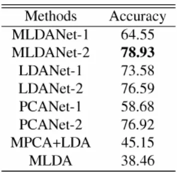
extract-Methods Accuracy MLDANet-l 64.55 MLDANet-2 78.93 LDANet-l 73.58 LDANet-2 76.59 PCANet-l 58.68 PCANet-2 76.92 MPCA+LDA 45.15 MLDA 38.46

Table 1. The best performance of MLDANet, LDANet, P­ CANet, MPCA+LDA and MLDA.

ed from MLDA vary from 10 to 100. We draw the recog­ nition accuracy of MPCA+LDA and MLDA in Fig. 4(d). The best performance of MLDANet, PCANet, LDANet, MP­ CA+LDA, and MLDA are listed in Table 1.

We see that all one-stage networks outperform two con­ ventional tensor object classification algorithms, that is, M­ PCA+LDA and MLDA. The reason is that the convolution­ al architecture imitate the brain networks, which can provide more robust feature than other methods for visual content [4]. LDANet-l achieves the best performance in the one-stage networks, but the improvement from LDANet-l to LDANet-2 is not larger as that ofMLDANet. PCANet-l performs worse than those based on LDA algorithm networks like LDANet and MLDANet. It is because that LDA type algorithm pro­ vides the features which have the best classification perfor­ mance, however, PCA maximize the directional variation in the features. MLDANet-l is not as good as LDANet-l be­ cause the feature extracted from MLDANet-l is not appropri­ ate as the direct input of linear SVM. For two-stage network­ s, MLDANet-2 achieves the best performance. Surprisingly, the performance of PCANet-2 increase not more than 18.24% compared to that of PCANet-l, but it is better than that of LDANet-2.

5. CONCLUSION

In this paper, we have proposed and implemented a novel deep learning architecture, that is, MLDANet, which takes full advantage of the structure information in tensor objects by convolutional architecture. MLDANet is composed of t­ wo convolutional layers, which use MLDA and LDA to learn filter banks respectively and one pooling layer. We have e­ valuated the performance of the MLDANet on UCFll and show that our model performs well in tensor object classifica­ tion. This work provides the inspiration for other convolution­ al deep architectures in tensor object classification. As future works, we will focus on the tensorial extension of CNN.

6. REFERENCES

[1] Y. _{Bengio, "Learnin.,.g deep architectures for AI, "} Foun­ dations and trends _® in Machine Learning, vol. 2, pp. 1-127, 2009.

[2] Y. LeCun, L. Bottou, Y. Bengio, and P. Haffner, "Gradient-based learning applied to document recogni­ tion, " Proceedings of the IEEE, vol. 86, pp. 2278-2324, 1998.

[3] A. Krizhevsky, I. Sutskever, and G.E. Hinton, "Image net classification with deep convolutional neural networks, " in Proceedings of NIPS , 2012, pp. lO97-11 05.

[4] Y. LeCun and Y. Bengio, "Convolutional networks for images, speech, and time series, " The handbook of brain theory and neural networks, vol. 3361, 1995.

[5] T.H. Chan, K Jia, S. Gao, J. Lu, Z. Zeng, and Y. Ma, "P­ canet: A simple deep learning baseline for image classi­ fication?, " arXiv preprint arXiv:i404.3606, 2014. [6] G. Shakhnarovich and B. Moghaddam, "Face recogni­

tion in subspaces, " Handbook of Face Recognition, pp. 19-49, 2011.

[7] D. Yu, L. Deng, and F. Seide, "The deep tensor neu­ ral network with applications to large vocabulary speech recognition, " IEEE Transactions on Audio, Speech, and Language Processing, vol. 21, pp. 388-396, 2013. [8] B. Hutchinson, L. Deng, and D. Yu, 'Tensor deep s­

tacking networks, " IEEE Transactions on Pattern Anal­ ysis and Machine intelligence, vol. 35, pp. 1944-1957, 20l3.

[9] "UCF11, " http: //crcv.ucf.edu/data/.

[lO] H. Lu, KN. Plataniotis, and A.N. Venetsanopoulos, "Uncorrelated multilinear discriminant analysis with regularization and aggregation for tensor object recog­ nition, " IEEE Transactions on Neural Networks, vol. 20, pp. 103-123, 2009.

[11] H. Lu, KN. Plataniotis, and A.N. Venetsanopoulos, "M­ pca: Multilinear principal component analysis of tensor objects, " iEEE Transactions on Neural Networks, vol. 19, pp. 18-39, 2008.