Task-based Conjugate Gradient: from multi-GPU towards heterogeneous architectures

HAL Id: hal-01316982

https://hal.inria.fr/hal-01316982v2

Submitted on 15 Dec 2016

HAL is a multi-disciplinary open access

archive for the deposit and dissemination of

sci-entific research documents, whether they are

pub-lished or not. The documents may come from

teaching and research institutions in France or

abroad, or from public or private research centers.

L’archive ouverte pluridisciplinaire HAL, est

destinée au dépôt et à la diffusion de documents

scientifiques de niveau recherche, publiés ou non,

émanant des établissements d’enseignement et de

recherche français ou étrangers, des laboratoires

publics ou privés.

Task-based Conjugate Gradient: from multi-GPU

towards heterogeneous architectures

E Agullo, L Giraud, A Guermouche, S Nakov, Jean Roman

To cite this version:

E Agullo, L Giraud, A Guermouche, S Nakov, Jean Roman. Task-based Conjugate Gradient: from

multi-GPU towards heterogeneous architectures. [Research Report] RR-8912, Inria. 2016.

�hal-01316982v2�

ISSN 0249-6399 ISRN INRIA/RR--8912--FR+ENG

RESEARCH

REPORT

N° 8912

Task-based Conjugate

Gradient: from

multi-GPU towards

heterogeneous

architectures

RESEARCH CENTRE BORDEAUX – SUD-OUEST

200 avenue de la Vielle Tour 33405 Talence Cedex

multi-GPU towards heterogeneous

architectures

E. Agullo

, L. Giraud

, A. Guermouche

, S. Nakov

, J. Roman

Project-Teams HiePACS

Research Report n° 8912 — May 2016 — 14 pages

Abstract: Whereas most parallel High Performance Computing (HPC) numerical libaries have

been written as highly tuned and mostly monolithic codes, the increased complexity of modern architectures led the computational science and engineering community to consider more mod-ular programming paradigms such as task-based paradigms to design new generation of parallel simulation code; this enables to delegate part of the work to a third party software such as a runtime system. That latter approach has been shown to be very productive and efficient with compute-intensive algorithms, such as dense linear algebra and sparse direct solvers. In this study, we consider a much more irregular, and synchronizing algorithm, namely the Conjugate Gradi-ent (CG) algorithm. We propose a task-based formulation of the algorithm together with a very fine instrumentation of the runtime system. We show that almost optimum speed up may be reached on a multi-GPU platform (relatively to the mono-GPU case) and, as a very preliminary but promising result, that the approach can be effectively used to handle heterogenous architec-tures composed of a multicore chip and multiple GPUs. We expect that these results will pave the way for investigating the design of new advanced, irregular numerical algorithms on top of runtime systems.

Key-words: High Performance Computing (HPC); multi-GPUs; heterogeneous architectures ;

task-based model; runtime system; sparse linear systems; Conjugate Gradient.

Implantation du gradient conjugué en tâches: du

multi-GPU aux architetures hétérogènes

Résumé : Alors que la majorité des librairies numériques pour le calcul intensif a été

écrite et optimisée essentiellement comme des codes monolitiques, le complexité croissante des architecture modernes a conduit la communité des sciences computationnelles à considérer des paradigmes de programmation plus modulaires, tel que la programmation à based de tâches, pour le design de la nouvelle génération des codes de calcul. Ceci permet en particulier de déléguer un partie du travail à une couche logicielle tierce qui est un support d’exécution à base de tâches. Cette approche s’est révélée extrèmement productive et efficace pour des noyaux de calcul tels que les solveurs linéaires denses et creux. Dans cette étude, nous considérons une méthode de résolution beaucoup plus irrégulière et synchronisante: le gradient conjugué. Nous proposons une formulation en tâches de cet algorihtme et montrons des résultats de performance quasi-optimaux sur une plateforme multi-GPU ainsi que des résultats préliminaires prometteurs sur une architecture hétérogène.

Mots-clés : Calcul Haute performance (HPC); multi-GPUs; architectures hétérogènes; modéle

1

Introduction

In the last decade, the architectural complexity of High Performance Computing (HPC) plat-forms has strongly increased. To cope with this complexity, programming paradigms are being revisited. Among others, one major trend consists of writing the algorithms in terms of task graphs and delegating to a runtime system both the management of the data consistency and the orchestration of the actual execution. This paradigm has been first intensively studied in the context of dense linear algebra [1, 2, 3, 6, 7, 8, 11, 12] and is now a common utility for related state-of-the-art libraries such as PLASMA, MAGMA, FLAME, DPLASMA and Chameleon. Dense linear algebra algorithms were indeed excellent candidates for pioneering in this direction. First, their regular computational pattern allows one to design very wide task graphs so that many computational units can execute tasks concurrently. Second, the building block operations they rely on, essentially level-three Basic Linear Algebra Subroutines (BLAS), are compute inten-sive, which makes it possible to split the work in relatively fine grain tasks while fully benefiting from GPU acceleration. As a result, these algorithms are particularly easy to schedule in the sense that state-of-the-art greedy scheduling algorithms may lead to a performance close to the optimum, including on platforms accelerated with multiple Graphics Processing Units (GPUs). Because sparse direct methods rely on dense linear algebra kernels, a large effort has been made to turn them into task-based algorithms [9, 4].

In this paper, we tackle another class of algorithms, the Krylov subspace methods, which aim at solving large sparse linear systems of equations of the form Ax = b, where A is a sparse matrix. Those methods are based on the calculation of approximated solutions in a sequence of embedded spaces, that is intrinsically a sequential numerical scheme. Second, their unpreconditioned versions are exclusively based on non compute intensive kernels with irregular memory access pattern, Sparse Matrix Vector products (SpMV) and level-one BLAS, which need very large grain tasks to benefit from GPU acceleration. For these reasons, designing and scheduling Krylov subspace methods on a multi-GPUs platform is extremely challenging, especially when relying on a task-based abstraction which requires to delegate part of the control to a runtime system. We discuss this methodological approach in the context of the Conjugate Gradient (CG) algorithm on a shared-memory machine accelerated with multiple GPUs using the StarPU runtime system [5] to process the designed task graph. The CG solver is a widely used Krylov subspace method, which is the numerical algorithm of choice for the solution of large linear systems with symmetric positive definite matrices [13].

The objective of this study is not to optimize the performance of CG on an individual GPU, which essentially consists of optimizing the matrix layout in order to speed up SpMV. We do not either consider the opportunity of reordering the matrix in order to improve the SpMV. Finally, we do not consider numerical variants of CG which may exhibit different parallel patterns. These three techniques are extremely important but complementary and orthogonal to our work. Instead, we rely on routines from vendor libraries (NVIDIA cuSPARSE and cuBLAS) to implement individual GPU tasks, we assume that the ordering is prescribed (we do not apply permutation) and we consider the standard formulation of the CG algorithm [13]. On the contrary, the objective is to study the opportunity to accelerate CG on multiple GPUs by designing an appropriate task flow where each individual task is processed on one GPU and all available GPUs are exploited to execute these tasks concurrently. We first propose a natural task-based expression of CG. We show that such an expression fails to efficiently accelerate CG. We then propose successive improvements on the task flow design to alleviate the synchronizations, exhibit more parallelism (wider graph) and reduce the volume of exchanges between GPUs.

The rest of the paper is organized as follows. We first propose a natural task-based expression of CG in Section 2. We then present the experimental set up in Section 3. We then show how the

4 Agullo et al. 1: r ← b 2: r ← r − Ax 3: p ← r 4: δnew← dot(r, r) 5: δold← δnew

6: for j = 0, 1, ...,until kb−Axk_kbk ≤ eps do

7: q ← Ap /* SpMV */

8: α ← dot(p, q) /* dot */

9: α ← δnew/α /* scalar operation

*/

10: x ← x + αp /* axpy */

11: r ← r − αq /* axpy */

12: δnew← dot(r, r)/* dot */

13: β ← δnew/δold /* scalar operation

*/

14: δold← δnew /* scalar operation

*/ 15: p ← r + βp /* scale-axpy */ 16: end for (a) Algorithm. SpMV SpMV SpMV dot dot Scal op axpy axpy axpy Scal op scal-axpy scal-axpy scal-axpy Line 7 Line 8 Line 9 Line 10 Line 11 Line 13, 14 Line 15 dot axpy axpy axpy scal-axpy scal-axpy scal-axpy SpMV SpMV SpMV dot dot dot axpy axpy axpy axpy axpy axpy dot dot Line 12 dot dot dot dot Unpartitioning Partitioning (b) Task-flow.

Figure 1: Conjugate Gradient (CG) linear solver.

baseline task-based expression can be enhanced for efficiently pipelining the execution of the tasks in Section 4. We present a performance analysis of a multi-GPU execution in Section 5. Section 6 presents concluding remarks together with preliminary experiments in the fully heterogeneous case.

2

Baseline Sequential Task Flow (STF) Conjugate Gradient

algorithm

In this section, we present a first task-based expression of the CG algorithm whose pseudo-code is given in Algorithm 1a. This algorithm can be divided in two phases, the initialization phase (lines 1-5) and the main iterative loop (lines 6-16). Since the initialization phase is executed only once, we only focus on an iteration occurring in the main loop in this study.

Three types of operations are used in an iteration of the algorithm: SpMV (the sparse matrix-vector product, line 7), scalar operations (lines 9, 13, 14) and level-one BLAS operations (lines 8, 10, 11, 12, 15). In particular three different level-one BLAS operations are used: scalar product (dot, lines 8 and 12), linear combination of vectors (axpy, lines 10, 11 and 15) and scaling of a vector by a scalar (scal, line 15). The scal kernel at line 15 is used in combination with an

axpy. Indeed, in terms of BLAS, the operation p ← r + βp consists of two successive operations:

p ← βp (scal) and then p ← r + p (axpy). In our implementation, the combination of these

level-one BLAS operations represents a single task called scale-axpy. The key operation in an iteration is the SpMV (line 7) and its efficiency is thus critical for the performance of the whole algorithm.

According to our STF programming paradigm, data need to be decomposed in order to provide opportunities for executing concurrent tasks. We consider a 1D decomposition of the

sparse matrix, dividing the matrix in multiple block-rows. The number of non-zero values per block-rows is balanced and the rest of the vectors follows the same decomposition.

After decomposing the data, tasks that operate on those data can be defined. The tasks derived from the main loop of Algorithm 1a are shown in Figure 1b, when the matrix is divided in six block-rows. Each task is represented by a box, named after the operation executed in that task, and edges represent the dependencies between tasks.

The first instruction executed in the main loop of Algorithm 1a is the SpMV . When a 1D decomposition is applied to the matrix, dividing it in six parts implies that six tasks are submitted

for this operation (the green tasks in Figure 1b): qi ← Aip, i ∈ [1, 6]. For these tasks, a copy

of the whole vector p is needed (vector p is unpartitioned). But in order to extract parallelism of other level-one BLAS operations where vector p is used (lines 8 and 15 in Algorithm 1a), in respect with our programming, the vector p needs to be partitioned. The partitioning operation is a blocking call; it thus represents a synchronization point in this task flow. Once vector p is partitioned, both vectors p and q are divided in six parts. Thus six dot tasks are submitted. Each

dot operation accesses α in read-write mode, which induces a serialization of the operation. This

sequence thus introduces new synchronizations in the task flow each time we need to perform a

dot operation. The twelve axpy tasks (six at line 10 and six at line 11) can then all be executed

in parallel. Another dot operation is then performed (line 12) and induces another serialization point. After the scalar operations at lines 13 and 14 in Algorithm 1a, the last scale-axpy operation of the loop is executed, which updates the vector p. At this stage, the vector is partitioned in six pieces. In order to perform the SpMV tasks for the next iteration, an unpartitioned version of the vector p is needed. This is done with the unpartition operation, similar to the partition operation, which is a blocking call.

All in all, this task flow contains four synchronization points per iteration, two for the par-tition/unpartition operation and two issued from the dot operations. The task flow is also very thin. Section 4.1 exhibits the induced limitation in terms of pipelining, while Sections 4.2, 4.3 and 4.4 propose successive improvements allowing us to alleviate the synchronizations and design a wider task flow, thus increasing the concurrency and the performance.

3

Experimental setup

All the tests presented in Section 5 have been run on a cache coherent Non Uniform Memory Access (ccNUMA) machine with two hexa-core processors Intel Westmere Xeon X5650, each one having 18GB of RAM, for a total of 36GB. It is equipped with three NVIDIA Tesla M2070 GPUs, each one equipped with 6GB of RAM memory. The task-based CG algorithm proposed in Section 2 is implemented on top of the StarPU v1.2. We use the opportunity offered by StarPU to control each GPU with a dedicated CPU core.To illustrate our discussion we consider the matrices presented in Table 1. All needed data is prefetched to the target GPU before the execution and assement of all the results presented in this paper.

Scheduling and mapping strategy. As discussed in Section 2, the task flow derived from

Algorithm 1a contains four synchronization points per iteration and is very thin, ensuring only a very limited concurrency. Pipelining this task flow efficiently is thus very challenging. In particular, dynamic strategies that led to close to optimum scheduling in dense linear algebra [2] are not well suited here. We have indeed experimented such a strategy (Minimum Completion Time (MCT) policy), but all studied variants failed to achieve a very high performance. We have thus implemented a static scheduling strategy. We perform a cyclic mapping of the block-rows on the available GPUs in order to ensure load balancing.

6 Agullo et al.

Matrix name nnz N nnz/ N flop / iteration

11pts-256 183 M 17 M 11 2 G

11pts-128 23 M 2 M 11 224 M

Audi_kw 154 M 943 K 163 317 M

af_0_k101 18 M 503 K 34 38 M

Table 1: Overview of sparse matrices used in this study. The 11pts-256 and 11pts-128 matrices are obtained from a 3D regular grid with 11pt discretization stencil. The Audi_kw and af_0_k101 matrices come from structural mechanics simulations on irregular finite element 3D meshes.

Building block operations. In order to explore the potential parallelism of the CG algorithm,

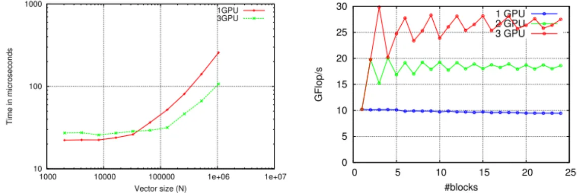
we first study the performance of its building block operations, level-one BLAS and SpMV . The granularity does not penalize drastically the performance for SpMV operation. Additionally when three GPUs are used, a speed-up of 2.93 is obtained. On the other hand, in order to efficiently exploit multiple GPUs, vector with sizes of at least few millions are needed.

10 100 1000 1000 10000 100000 1e+06 1e+07 Time in microseconds Vector size (N) 1GPU 3GPU

(a) Performance of the axpy kernel. The rest of the BLAS-1 kernels follow the same behavior.

0 5 10 15 20 25 30 0 5 10 15 20 25 GFlop/s #blocks 1 GPU 2 GPU 3 GPU

(b) Performance of the SpMV kernel on the Audi_kw matrix.

Figure 2: Performance of the building block operations used in the CG algorithm. All data is prefetched before execution and performance assessment.

4

Achieving efficient software pipelining

In accordance with the example discussed in Section 2, the matrix is split in six block-rows and three GPUs are used. We pursue our illustration with matrix 11pts-128.

4.1

Assessment of the proposed task-based CG algorithm

Figure 3 shows the execution trace of one iteration of the task flow (Figure 1b) derived from Algorithm 1a with respect to the mapping proposed in Section 3. Figure 3 can be interpreted as follows. The top black bar represents the state of the CPU RAM memory during the execution. Each GPU is represented by a pair of bars, one for the state of the GPU and the black bar which

depicts the memory state of the GPU. When data movement occurs between different memory nodes, they are highlighted by an arrow from the source to the destination. The top bar for each GPU represents its activity. The activity of a GPU may have one of the three following states: active computation (green), idle (red) or active waiting for the completion of a data transfer (purple).

Figure 3: Execution trace of an iteration with the CG task flow of Figure 1b using three GPUs. An iteration starts with the execution of a SpMV operation (line 7 in Algorithm 1a) which

corresponds time interval [t0,t1] in Figure 3. Following the cyclic mapping strategy presented

in Section 3, each GPU is thus in charge of two SpMV tasks. At time t1, the vector p is

unpartitioned. The vector p is partitioned into six pipieces, i ∈ [1, 6], with respect to the

block-row decomposition of the matrix. However, this data partitioning operation is a blocking call (see Section 2) which means that no other task can be submitted until it is completed at time

t1(the red vertical bar after the SpMV tasks in Figure 1b). Once vector p is partitioned, tasks

for all remaining operations (lines 8-15) are submitted. The dot tasks are executed sequentially with respect to the cyclic mapping strategy. The reason for this, as explained in Section 2, is that the scalar α is accessed in read-write mode. In addition, α needs to be moved to GPUs

between each execution of a dot task (time interval [t1, t2] in Figure 3). Once the scalar product

at line 8 is computed, the scalar division follows (line 9) executed on GPU 1 (respecting the task flow in Figure 1b). The execution of the next two instructions follows (lines 10 and 11). But before the beginning of the execution of the axpy tasks on GPU 2 and GPU 3, the new value of

αis sent (the purple period at t2 in Figure 3). The axpy tasks (yellow tasks in Figure 1b) are

then executed during the period [t2, t3] in parallel. The scalar product at line 12 is then executed

during the time interval [t3, t4], following the same sequence as explained above for line 8. Next,

βand δoldare computed on GPU 1 at time t4in Figure 3, representing the scalar operations from

lines 13 and 14 of Algorithm 1a. Tasks related to the last operation of the iteration (scale-axpy

tasks in Figure 1b) are then processed during the time interval [t4,t5]. When all the new vector

blocks piare calculated, the vector p is unpartitioned (red vertical bar after the scale-axpy tasks

in Figure 1b). As explained in Section 2, this data unpartition is another synchronization point

and may only be executed in the RAM. All blocks pi of vector p are thus moved by the runtime

system from the GPUs to the RAM during the time interval [t5,t6] for building the unpartitioned

vector p. This vector is then used to perform the qi← Ai× ptasks related to the first instruction

of the next iteration (SpMV at line 7). We now understand why the iteration starts with an

active waiting of the GPUs (purple parts before time t0): vector p is only valid in the RAM and

thus needs to be copied on the GPUs.

During the execution of the task flow derived from Algorithm 1a (Figure 1b), the GPUs are idle during a large portion of the time (red and purple parts in Figure 3). In order to achieve more efficient pipelining of the algorithm, we present successive improvements on the design of the task flow: relieving synchronization points (Section 4.2), reducing volume of communication that is achieved using a packing data mechanism (Section 4.3) and relying on a 2D decomposition (Section 4.4).

8 Agullo et al.

4.2

Relieving synchronization points

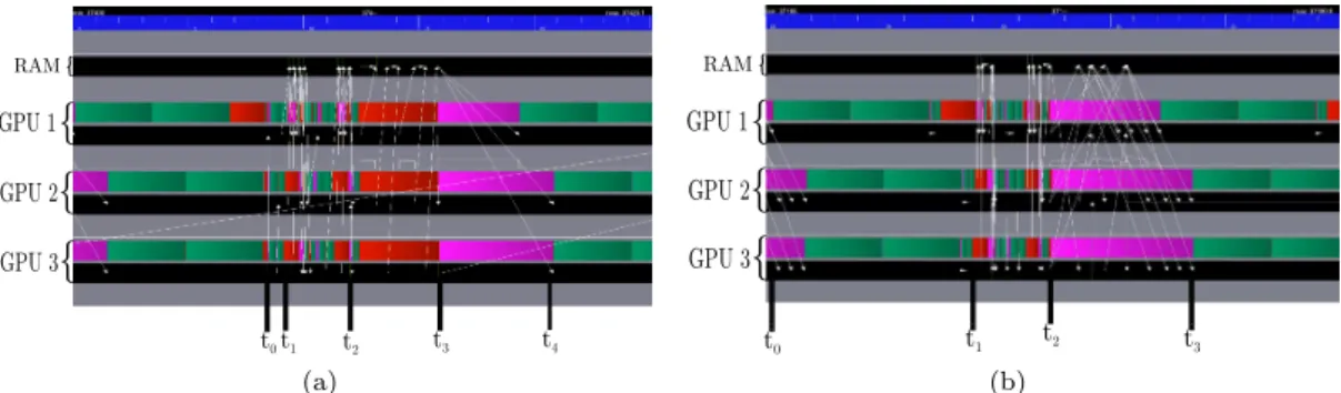
Alternatively to the sequential execution of the scalar product, each GPU j can compute locally

a partial sum (αj_{) and perform a StarPU reduction to compute the final value of the scalar}

(α = Pn_gpus

j=1 α

j_{). Figure 4a illustrates the benefit of this strategy. The calculation of the}

scalar product, during the time interval [t0, t1] is now performed in parallel. Every GPU is

working on its own local copy of α and once they have finished, the reduction is performed on

GPU 1 just after t1.

t0t1 t2 t3 t4 RAM{ GPU 1

{

{

{

{

{

{

Figure 4: Execution trace of one iteration when the dot is performed in reduction mode (left) and after furthermore avoiding data partitioning and unpartitioning (right).

The partition (after instruction 7 of Algorithm 1a) and unpartition (after instruction 15) of vector p, that are special features of StarPU, represent two of the four synchronization points within each iteration. They furthermore induce extra management and data movement costs. Indeed, after instruction 15, each GPU owns a valid part of vector p. For instance, once GPU 1

has computed p1, StarPU moves p1 to the RAM and then receives it back. Second, vector p has

to be fully assembled in the main memory (during the unpartition operation) before prefetching

a copy of the fully assembled vector p back to the GPUs (after time t3 in Figure 4a). We have

designed another scheme where vector p is kept by StarPU in a partitioned form all along the execution (it is thus no longer needed to perform partitioning and unpartitioning operations at each iteration). Instead of building and broadcasting the whole unpartitioned vector p, each GPU gathers only the missing pieces. This enables us to “remove” the two synchronization points related to the partition and unpartition operations, since they are not called anymore, and decrease the overall traffic. Figure 4b illustrates the benefits of this policy. Avoiding the unpartitioning operation allows us to decrease the time required between two successive iterations from 8.8 ms to 6.6 ms. Furthermore, since the partitioning operation is no longer needed, the corresponding synchronization in the task flow control is removed. The corresponding idle time

(red part at time t0 in Figure 4a) is removed and instructions 7 and 8 are now pipelined (period

[t0,t1] in Figure 4b).

Coming back to Figure 4a, one may notice that GPUs are idle for a while just before time

t1 and again just before time t2. This is due to the reduction that finalizes each dot operation

(dot(p, q) at instruction 8 and dot(r, r) at instruction 12, respectively). In Algorithm 1a, vector

x is only used at lines 10 (in read-write mode) and 6 (in read-only mode). The execution of

instruction 10 can thus be moved anywhere within the iteration as long as the other input data of instruction 9, i.e. p and α have been updated to the correct values. In particular, instruction 10 can be moved after instruction 12. This delay enables StarPU to overlap the final reduction of

the dot occurring at instruction 12 with the computation of vector x. The red part before t2

in Figure 4a becomes (partially) green in Figure 4b. The considered CG formulation does not provide a similar opportunity to overlap reduction finalizing the dot operation at instruction 8.

4.3

Reducing communication volume by packing data

By avoiding data partition and data unpartition operations, the broadcast of vector p has been

improved (from period [t2, t4] in Figure 4a to period [t3, t4] in Figure 4b), but still the

com-munication time remains the large performance bottleneck (time interval [t3, t4]in Figure 4b).

This volume of communication can be decreased. Indeed, if a column within the block-row Aiis

zero, then the corresponding entry of p is not involved in the computation of the task qi← Aip.

Therefore, p can be pruned.

RAM{ GPU 1

{

{

{

{

{

{

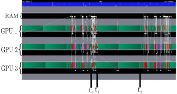
Figure 5: Execution trace when furthermore the vector p is packed.

We now explain how we can achieve a similar behavior with a task flow model. Instead of letting StarPU broadcast the whole vector p on every GPU, we can define tasks that only transfer the required subset. Before executing the CG iterations, this subset is identified with a symbolic

preprocessing step. Based on the structure of the block Ai,j, we determine which part of pj is

needed to build qi. If pj is not fully required, we do not transfer it directly. Instead, it can be

packed into an intermediate data, pi,j. StarPU provides an elegant support for implemented all

these advanced techniques through the definition of new data types. We rely on that mechanism for implementing this packing scheme. Furthermore, the packing operation may have a non

negligible cost whereas sometimes the values of pi,j that needs to be sent are almost contiguous.

In those cases, it may thus be worth sending an extra amount of data in order to directly send the

contiguous superset of pi,j ranging from the first to the last index that needs to be transferred.

We have implemented such a scheme. A preliminary tuning is performed for each matrix and

for each pi,j block to choose whether pi,j is packed or transferred in a contiguous way. Although

StarPU can perform automatic prefetching, the prefetching operation is performed once all the dependencies are satisfied. In the present context, with the static mapping, this may be too late and further anticipation may be worthy. Therefore, we help the runtime system in performing data prefetching as soon as possible performing explicit prefetching within the callback of the

scale-axpy task. We also do so after the computation of the α and β scalar values (lines 9 and

13 in Algorithm 1a) for broadcasting them on all GPUs.

Figure 5 depicts the execution trace. The time interval [t3, t4] in Figure 4b needed for the

broadcasting of the vector p has been reduced to the interval [t0, t1] in Figure 5. In the rest

of the paper we refer to as the full algorithm when all the blocks are transferred, or to as the

packedalgorithm if this packing mechanism is used.

10 Agullo et al. RAM{ GPU 1

{

{

{

{

{

{

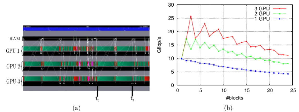
Figure 6: Execution trace when relying of a 2D decomposition of the matrix (left) and the performance of SpMV kernel when 2D decompostion is applied to the matrix (right).

4.4

2D decomposition

The 1D decomposition scheme requires that for each SpMV task, all blocks of vector p (packed or not packed) are in place before starting the execution of the task. In order to be able to

overlap the time needed for broadcasting the vector p (time interval [t0, t1] in Figure 5), a 2D

decomposition must be applied to the matrix. The matrix is first divided in block-rows, and then the same decomposition is applied to the other dimension of the matrix. Similarly as for a 1D decomposition, all the tasks SpMV associated with the entire block-row will be mapped on the same GPU. Contrary to the 1D decomposition, where we had to wait for the transfer of all missing blocks of the vector p, with the 2D decomposition, time needed for the transfer of the vector p can be overlapped with the execution of the SpMV tasks for which the blocks of the vector p are already available on that GPU. On the other hand, the 2D SpMV tasks yield lower performance then 1D (see Figure 6b and 2b), since they are executed on lower granularity.

The result of the impact of a 2D decomposition is shown in Figure 6a. During the time

interval [t1, t2] in Figure 5 there is no communication, while in Figure 6a communications are

overlapped with the execution of the SpMV tasks. In the rest of the paper we refer to either 1D or 2D depending on the data decomposition used. The trade-off between large task granularity (1D) and increased pipeline (2D) will be discussed in Section 5.

5

Performance analysis

We now perform a detailed performance analysis of the task-based CG algorithm designed above. We propose to analyze the behavior of our algorithms in terms of speed-up (S) and parallel efficiency (e) with respect to the execution occurring on one single GPU. In order to understand in more details the behavior of the proposed algorithms, we decompose the parallel efficiency into three effects, following the methodology proposed in [10]: the effect of operating at a lower

granularity (egranularity), the effect of concurrency on the performance of individual tasks (etasks)

and the effect of achieving a high task pipeline (epipeline). As shown in [10], the following equality

holds:

e = egranularity× etasks× epipeline.

We observed that the efficiency of the task is maximum (etasks = 1). Indeed, in a multi-GPU context, the different workers do not interfere with each other (they do not share memory or caches) and hence do not deteriorate the performance of one another. In the sequel, we thus

only report on egranularity and epipeline.

1D 2D 1D 2D

# GPUs full pack. full pack. full pack. full pack.

11pts-256 11pts-128 1 9.74 9.58 2 12.33 19.10 16.66 17.24 11.5 17.6 14.3 16.1 3 11.70 28.39 13.26 23.17 9.01 24.2 9.22 20.6 Audi_kw af_0_k101 1 10.0 9.84 2 15.6 15.6 16.3 16.7 12.1 16.3 13.6 15.0 3 17.7 20.0 22.0 23.6 11.1 19.4 12.5 18.2

Table 2: Performance (in Gflop/s) of our CG algorithm for the matrix collection presented in Table 1.

Table 2 presents the performance achieved for all matrices in our multi-GPU context. The optimal performance is represented for each scheme in bold value. The first thing to be observed is that for all the matrices, the pack version of our algorithm where only just the needed part of the vector p is broadcasted, yields the optimal performance. Broadcasting entire sub-blocks is too expensive and thus considerably slows down the execution of the CG algorithm. For the matrices that have a regular distribution of the non zeros, i.e. the 11pts-256, 11pts-128 and the af_0_k101 matrices, the 1D algorithm outperforms the 2D algorithm. On the other hand, in the case of the Audi_kw matrix that has an unstructured pattern, the 2D algorithm which exhibits more parallelism, yields the best performance.

Matrix 11pts-256 11pts-128 Audi_kw af_0_k101

S 2.91 2.52 2.36 1.97

e 0.97 0.84 0.79 0.65

egranularity 0.99 0.98 0.87 0.96

epipeline 0.97 0.86 0.91 0.68

Table 3: Obtained speed-up (S), overall efficiency (e), effects of granularity on efficiency

egranularity and effects of pipeline on efficiency epipeline for matrices presented in Table 1 on

3 GPUs.

Table 3 allows for analyzing how the overall efficiency is decomposed according to the metrics proposed above. Dividing the 11pts-256 matrix in several block-rows does not induce a penalty

on the task granularity (egranularity= 0.99 ≈ 1). Furthermore, thanks to all the improvements of

the task flow proposed in Section 4, a very high pipeline efficiency is achieved (epipeline= 0.97),

12 Agullo et al. leading to an overall efficiency of the same (very high) magnitude. For the 11pts-128 matrix,

the matrix decomposition induces a similar granularity penalty egranularity = 0.98. The slightly

lower granularity efficiency is a direct consequence of the matrix order. For smaller matrices, the tasks are performed on smaller sizes, thus the execution time per task is decreased. This makes our algorithm more sensitive to the overhead created by the communications induced by the dot-products and the broadcasting of the vector p, ending up with a less optimal (but still

high) pipeline efficiency (epipeline = 0.86). The overall efficiency for this matrix is e = 0.84.

This phenomenon is amplified when the matrix order is getting lower, such as in the case of the

af_0_k101matrix, resulting in a global efficiency of e = 0.65. The Audi_kw matrix yields optimal

performance with the 2D algorithm (see Section 4.4). Although the 2D algorithm requires to split

the matrix in many more blocks inducing a higher penalty on granularity (egranularity= 0.87), it

allows for a better overlap of communication with computation ensuring that a higher pipeline

(epipeline = 0.91) is achieved. With this trade-off, an overall efficiency equal to e = 0.79 is

obtained.

6

Towards a fully heterogeneous CG solver

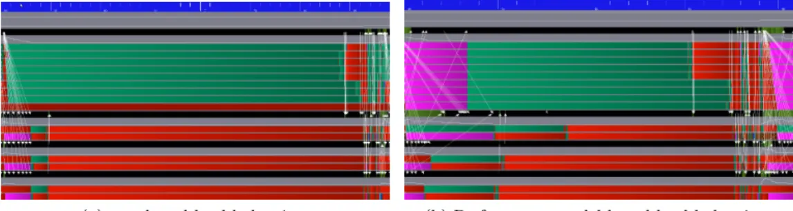
(a) nnz-based load balancing. (b) Performance model-based load balancing.

Figure 7: Traces of an execution of one iteration of the CG algorithm in the heterogeneous case (9 CPU and 3 GPU workers) with different partitioning strategies for the Audi_kw matrix. In 7a, the nnz is balanced per block-row (33µs). In 7b a feed-back from a history based performance model is used for the partitioning of the matrix (16µs).

One advantage of relying on task-based programming is that the architecture is fully ab-stracted. We prove here that we can benefit from this design to run on an heterogeneous node composed of all available computational resources. Because the considered platform has 12 CPU cores and three GPUs, but that each GPU has a CPU core dedicated to handle it, we can only rely on 9 CPU workers and 3 GPU workers in total.

Figure 7 presents execution traces of preliminary experiments that rely on two different strategies for balancing the load between CPU cores and GPU. These traces show the ability of task-based programming in exploiting heterogeneous platforms. However, they also show that more advanced load balancing strategies need to be designed in order to achieve a better occupancy. This question has not been fully investigated yet and will be further investigated in a future work.

7

ACKNOWLEDGEMENT

The authors acknowledge the support by the INRIA-TOTAL strategic action DIP1_{and especially}

Henri Calandra who closely followed this work.

References

[1] Emmanuel Agullo, Cédric Augonnet, Jack Dongarra, Mathieu Faverge, Julien Langou, Hatem Ltaief, and Stanimire Tomov. LU factorization for accelerator-based systems. In Howard Jay Siegel and Amr El-Kadi, editors, The 9th IEEE/ACS International Conference on Computer Systems and Applications, AICCSA 2011, Sharm El-Sheikh, Egypt, December

27-30, 2011, pages 217–224. IEEE, 2011.

[2] Emmanuel Agullo, Cédric Augonnet, Jack Dongarra, Mathieu Faverge, Hatem Ltaief, Samuel Thibault, and Stanimire Tomov. QR Factorization on a Multicore Node Enhanced with Multiple GPU Accelerators. In IPDPS, pages 932–943. IEEE, 2011.

[3] Emmanuel Agullo, Cédric Augonnet, Jack Dongarra, Hatem Ltaief, Raymond Namyst, Samuel Thibault, and Stanimire Tomov. Faster, Cheaper, Better – a Hybridization Method-ology to Develop Linear Algebra Software for GPUs. In Wen mei W. Hwu, editor, GPU

Computing Gems, volume 2. Morgan Kaufmann, September 2010.

[4] Emmanuel Agullo, Alfredo Buttari, Abdou Guermouche, and Florent Lopez. Implementing multifrontal sparse solvers for multicore architectures with Sequential Task Flow runtime systems. ACM Transactions On Mathematical Software, 2016. To appear.

[5] Cédric Augonnet, Samuel Thibault, Raymond Namyst, and Pierre-André Wacrenier. StarPU: A Unified Platform for Task Scheduling on Heterogeneous Multicore Architec-tures. Concurrency and Computation: Practice and Experience, Special Issue: Euro-Par

2009, 23:187–198, February 2011.

[6] George Bosilca, Aurelien Bouteiller, Anthony Danalis, Mathieu Faverge, Azzam Haidar, Thomas Hérault, Jakub Kurzak, Julien Langou, Pierre Lemarinier, Hatem Ltaief, Piotr Luszczek, Asim YarKhan, and Jack Dongarra. Flexible Development of Dense Linear Alge-bra Algorithms on Massively Parallel Architectures with DPLASMA. In IPDPS Workshops, pages 1432–1441. IEEE, 2011.

[7] Alfredo Buttari, Julien Langou, Jakub Kurzak, and Jack Dongarra. Parallel tiled QR factor-ization for multicore architectures. Concurrency and Computation: Practice and Experience, 20(13):1573–1590, 2008.

[8] Jakub Kurzak, Hatem Ltaief, Jack Dongarra, and Rosa M. Badia. Scheduling dense linear algebra operations on multicore processors. Concurrency and Computation: Practice and

Experience, 22(1):15–44, 2010.

[9] Xavier Lacoste, Mathieu Faverge, Pierre Ramet, Samuel Thibault, and George Bosilca. Tak-ing advantage of hybrid systems for sparse direct solvers via task-based runtimes, 05/2014 2014.

[10] Stojce Nakov. On the design of sparse hybrid linear solvers for modern parallel architectures. Theses, Université de Bordeaux, December 2015.

1_{http://dip.inria.fr}

14 Agullo et al. [11] G. Quintana-Ortí, E. S. Quintana-Ortí, E. Chan, F. G. Van Zee, and R. A. van de Geijn. Scheduling of QR factorization algorithms on SMP and multi-core architectures. In

Pro-ceedings of PDP’08, 2008. FLAME Working Note #24.

[12] Gregorio Quintana-Ortí, Francisco D. Igual, Enrique S. Quintana-Ortí, and Robert A. van de Geijn. Solving dense linear systems on platforms with multiple hardware accelerators. ACM

SIGPLAN Notices, 44(4):121–130, April 2009.

[13] Y. Saad. Iterative Methods for Sparse Linear Systems. Society for Industrial and Applied Mathematics, Philadelphia, PA, USA, 2nd edition, 2003.

BORDEAUX – SUD-OUEST

200 avenue de la Vielle Tour 33405 Talence Cedex

Inria

Domaine de Voluceau - Rocquencourt BP 105 - 78153 Le Chesnay Cedex inria.fr