HAL Id: hal-01728776
https://hal.archives-ouvertes.fr/hal-01728776
Submitted on 12 Mar 2018
HAL is a multi-disciplinary open access
archive for the deposit and dissemination of
sci-entific research documents, whether they are
pub-lished or not. The documents may come from
teaching and research institutions in France or
abroad, or from public or private research centers.
L’archive ouverte pluridisciplinaire HAL, est
destinée au dépôt et à la diffusion de documents
scientifiques de niveau recherche, publiés ou non,
émanant des établissements d’enseignement et de
recherche français ou étrangers, des laboratoires
publics ou privés.
A three-dimensional experimental investigation of the
structure of the spanwise vortex generated by a shallow
vortex dipole
Julie Albagnac, Frédéric Moulin, Olivier Eiff, Laurent Lacaze, Pierre Brancher
To cite this version:
Julie Albagnac, Frédéric Moulin, Olivier Eiff, Laurent Lacaze, Pierre Brancher. A three-dimensional
experimental investigation of the structure of the spanwise vortex generated by a shallow vortex dipole.
Environmental Fluid Mechanics, Springer Verlag, 2014, 14 (5), pp.957-970.
�10.1007/s10652-013-9291-6�. �hal-01728776�
O
pen
A
rchive
T
OULOUSE
A
rchive
O
uverte (
OATAO
)
OATAO is an open access repository that collects the work of
Toulouse researchers and makes it freely available over the
web where possible.
This is an author-deposited version published in :
http://oatao.univ-toulouse.fr/
Eprints ID : 19651
To link to this article : DOI:10.1007/s10652-013-9291-6
URL :
http://dx.doi.org/10.1007/s10652-013-9291-6
To cite this version : Albagnac, Julie
and Moulin, Frederic Y.
and Eiff, Olivier
and Lacaze, Laurent
and Brancher,
Pierre
A three-dimensional experimental investigation of the
structure of the spanwise vortex generated by a shallow vortex
dipole. (2014) Environmental Fluid Mechanics, vol. 14 (n° 5). pp.
957-970. ISSN 1567-7419
Any correspondence concerning this service should be sent to the
repository administrator:
[email protected]
A three-dimensional experimental investigation
of the structure of the spanwise vortex generated
by a shallow vortex dipole
Julie Albagnac · Frederic Y. Moulin · Olivier Eiff · Laurent Lacaze · Pierre Brancher
Abstract The three-dimensional dynamics of shallow vortex dipoles is investigated by
means of an innovative three-dimensional, three-component (3D-3C) scanning PIV tech-nique. In particular, the three-dimensional structure of a frontal spanwise vortex is charac-terized. The technique allows the computation of the three-dimensional pressure field and the planar (x, y) distribution of the wall shear stress, which are not available using standard 2D PIV measurements. The influence of such a complex vortex structure on mass transport is discussed in the context of the available pressure and wall shear stress fields.
Keywords Shallow flows · Vortex dipole · 3D-3C scanning PIV · Vortex identification ·
Pressure-field· Mass transport
1 Introduction
Similar to continuously stratified flows, a flow is qualified as shallow if the length scale of the horizontal structures is large compared to the depth of the fluid [17,25]. It is commonly assumed as a first approximation that the vertical confinement tends to inhibit vertical motions. Shallow flows are therefore usually described as quasi-two-dimensional (Q2D), i.e., flows with mainly horizontal two-dimensional motions, but with strong vertical gradients [14,20]. The inhibition of vertical motions is also invoked to explain the self-organization of the flow into large coherent horizontal structures when, for example, an initially three-dimensional horizontal turbulent jet in a shallow homogeneous layer of fluid evolves into a large hor-izontal vortex dipole composed of two counter-rotating vortices in close interaction [23]. Vortex dipoles also occur in continuously stratified flows and are indeed ubiquitous coherent
J. Albagnac (
B
)· F. Y. Moulin · O. Eiff · L. Lacaze · P. BrancherINPT, UPS, Institut de Mécanique des Fluides de Toulouse, Université de Toulouse, Allée Camille Soula, 31400 Toulouse, France
e-mail: [email protected]
J. Albagnac· F. Y. Moulin · O. Eiff · L. Lacaze · P. Brancher
hydrodynamic structures in geophysical flows, motivating many studies in the past decades to investigate their dynamics, stability and transport properties.
The role of vortex dipoles in mass transport is illustrated by the study of [24], who inves-tigated the correlation between foraging trips of frigatebirds over the Mozambique Channel and the Lagrangian coherent structures at the free surface. They noticed that frigatebirds followed the contours of large vortex dipoles since they were favorable fishing areas. They concluded that vortex dipoles, which self-propagate over large distances, are associated to intense marine biological activity due to their ability to transport nutrients up to the free surface. Such vertical motions associated with vortex dipoles in shallow flow have also been observed through the coloration of water by sediments detached from the seabed and trans-ported to the free surface [6,15,18,21]. All these observations support the conjecture that vertical motions, though presumably negligible due to the vertical confinement in the frame-work of the Q2D approximation, could nevertheless be strong enough to play an important role in the mass transport induced by shallow water dipoles.
Several studies have recently addressed and challenged the question of the commonly assumed quasi-two-dimensionality of shallow water flows. Lin et al. [17] and Sous et al. [22,23] studied the formation of Q2D shallow vortex dipoles resulting from decaying tur-bulence. Nevertheless, subsequently to the formation of the vortex dipole, they observed a spanwise vortex at the front of the vortex dipole, which can therefore be attributed to the shallow vortex dipole dynamics over a solid bottom. Akkermans et al. [2] performed stereo-scopic PIV on electromagnetically forced shallow vortex dipoles. They noticed the presence of a similar spanwise vortex. Tentative explanations of the presence of a spanwise vortex in the above-mentioned studies invoked a self-organization of the initial three-dimensional turbulence [22,23] or the vertically non-homogeneous flow field generated by the electro-magnetic forcing [2]. In order to identify the physical origin of the observed spanwise vortex, [16] studied shallow vortex dipoles produced by a vertical flap apparatus forcing the flow homogeneously along the whole water depth. They observed a spanwise vortex at the front of the dipole, showing that an initially two-dimensional laminar shallow dipole is also able to evolve into a three-dimensional structure due to the stretching of the horizontal vorticity in the boundary layer below the dipole. Duran-Matute et al. [8] and Albagnac et al. [3] addressed the conditions under which the spanwise vortex is generated at the front of a shallow vortex dipole. For this purpose, numerical simulations and experiments on shallow vortex dipoles electromagnetically forced [8] and experiments using a flap apparatus [3] have been led for a wide range of water depths and dipole propagation velocities. They showed that the existence of the spanwise vortex depends on the non-dimensional parameter, α2Re, which takes into
account both the aspect ratio (or equivalently the vertical confinement) of the flow α= h/D (where h is the water depth and D is the diameter of the dipole) and the Reynolds number associated with the horizontal propagation velocity of the dipole Re= UD/ν (where U is the initial propagation velocity of the dipole and ν is the kinematic viscosity). When α2Reis
large enough, a spanwise vortex develops at the front of the vortex dipole independently of the way the shallow vortex dipole is generated. These experimental results were based on 2D slices of the flow, with access to the spanwise vorticity in the vertical symmetry plane of the vortex dipole. A better description and understanding of the three-dimensional, time evolving structure of the principal vortex dipole, and its connection and interaction with the growing spanwise vortex, requires access to well-resolved measurements of the three components of the vorticity in the complete volume of the flow. Such a complete 3D description of the flow, including the pressure and shear–stress fields, is the main motivation for the present study. The study is also expected to yield insight into the erosion and mass-transport potential of the complex vortex structure.
The experimental set-up and the three-dimensional, three-component (3D-3C) scanning particle image velocimetry (Scanning PIV) technique used for this study are described in Sect.2. The resulting complete three-dimensional measurement of the entire vortex dipole structure and its time evolution are shown in Sect.3. The time evolution of the pressure field and its gradient, also determined from the 3D-3C scanning PIV measurements, are presented in Sect.4. Section5then presents the analysis of the planar wall shear-stress field at the bottom. Finally, a summary of the results and the perspectives of this study are given in Sect.6.
2 Experimental set-up and 3D-3C scanning PIV measurements
2.1 Vortex dipole generator
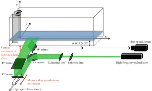
Vortex dipoles are generated by the closing of a pair of vertical flaps in a 2 m long, 1 m wide and 0.7 m deep tank filled with a layer of water of depth h = 35 mm initially at rest (Fig.1). The flap apparatus is the same device as the one used by Billant and Chomaz [4], Lacaze et al. [16] and Albagnac et al. [3]. A pair of vertical flaps, initially parallel to each other, is put into motion around the vertical axis such that the flaps rotate one towards the other. This generates two counter-rotating vortices, forming a vortex dipole which propagates away from the flaps by mutual induction. This experimental set-up has been chosen in order to generate laminar, regular and reproducible vortex dipoles characterized by three independent dimensional parameters, namely, their initial diameter D0, their initial propagating velocity
U0and the water depth h in which they evolve. This leads to two non-dimensional numbers:
the Reynolds number defined as Re = U0D0/ν(where ν is the kinematic viscosity of the water) and the aspect ratio of the flow defined as α= h/D0. The present study focuses on
a representative vortex dipole, leading to the generation of a frontal spanwise vortex, with α= 0.54 and Re=290 (α2Re = 84.5) with U0 = 4.5 mm s−1and h = 35 mm.
In the following, x, y and z denote the streamwise, spanwise, and vertical directions respectively. The origin of the x, y and z axes is located at the initial flap trailing edge, in the vertical symmetry plane and at the tank bottom (see Fig.1). The initial time t = 0 s corresponds to the end of the flaps rotation.
2.2 3D-3C scanning PIV set-up and technique
The 3D-3C scanning PIV technique is based on the work of [11,12], and has been developed in conjunction with [5]. The 3D-3C scanning PIV technique consists in acquiring two volumetric images of particles seeded in the flow by means of a 2D laser sheet which is rapidly translated in the normal, out of plane direction while a single camera images the successive illuminated planes during the scan. In this method, the time scale associated with the scanning has to be small compared to the time scale associated with the flow dynamics, in order to consider each reconstructed volume as instantaneous. The time interval between the acquisition of the two volumes is based on the flow dynamics as in standard 2D PIV techniques. On the basis of two such volumes, in direct analogy to two images in 2D PIV [10], a three-dimensional volumetric image correlation is performed in order to obtain the three velocity components in three dimensions as well as all their spatial derivatives.
The volumetric images are obtained by rapidly translating a horizontal laser sheet vertically throughout the desired depth of fluid (here the entire depth h) by means of a high-speed linear motor (X2502 by Copley motors), while acquiring synchronized sequential 2D horizontal
Fig. 1 Vortex dipole generation and 3D-3C scanning PIV set-up. The sketch is not at scale
images with a high-speed camera of overlapping slices of the flow illuminated by the moving laser sheet (see Fig.1). The camera (a 1,024× 1,024 pixels LaVision HighSpeedStar) is fixed in the laboratory and positioned far from the image-volume (here about 5 m) with a long focal-length lens (a Nikon 400 mm) in order to minimize parallax.
The laser sheet is generated with a 2× 22mJ (at 1,000Hz) dual cavity high frequency pulsed laser (Quantronix Darwin Duo) positioned with an optical path of about 5 m from the image volume. The two pulses are synchronized to obtain 44 m J of energy and the resulting beam is focused and collimated with several spherical lenses and widened in the horizontal direction with a cylindrical lens in order to create a light sheet in the image-volume of about 1.5 mm thickness and 30 cm width (for a 15 cm image width). As seen in Fig.1, the vertical motion of the laser sheet is obtained by the horizontal translation of a small 45◦first-surface
mirror mounted directly on the moving linear motor and a larger fixed 45◦ first-surface
mirror mounted above the motor. Images are taken from below the glass bottom of the tank via another 45◦first-surface mirror, allowing the camera to be placed as far as desired while
avoiding perturbations from the free-surface if the camera were positioned directly above. The motor electronics control the synchronization with the pulsed laser and the camera with a precision of 1 µs. The position of the motor is controlled via an optical rail with a precision of 5 µm.
The scanning speed and acceleration/deceleration are 0.17 m s−1and 150 m s−2, respec-tively, lower than the maximum available values of about 10 m s−1and 250 m s−2, designed to
accommodate higher speed flows and larger scanning volumes. The processed images were acquired at 500 Hz, yielding a vertical displacement between consecutive images of 0.34 mm. This vertical displacement is the vertical voxel (volumetric pixel, i.e., volume whose each face is a pixel) size. With the estimated laser-sheet thickness of 1.5 mm, a vertical displacement of 0.34 mm yields a theoretical image overlap ratio of 4.4. Analysis of the images revealed that a given particle is actually imaged in 3–4 consecutive images, implying that the effective sheet thickness is somewhat smaller. With a fluid depth h = 35 mm, 102 images were taken per volume.
The volumetric images are constructed by superposition of the consecutive 2D horizontal images, yielding a 3D image matrix with n× m × k voxels, where n × m is the image resolution (1024× 1024 pixels) and k is the number of superposed images (102). The imaging of particles in the horizontal plane is direct as the slices composing the volume are horizontal. In the vertical plane, the vertical intensity distribution of a given particle is given by the successive imaging of the particles due to the imposed vertical overlap combined with the vertically varying intensity of the laser sheet’s approximate Gaussian distribution. In other words, since the particles are effectively fixed in space, they will be illuminated with varying intensity in the successive positions of the laser sheet (here 3–4 levels or voxels) by its approximate Gaussian vertical intensity distribution.
Three to 4 Pixels is also approximately the size of the imaged particles in the 2D horizontal images themselves such that the 3D image particle resolution is approximately isotropic with a size of about 33to 43voxels. As mentioned above, the vertical voxel size is 0.34 mm while
the horizontal voxel size, obtained via calibration plates in the center of the image volume, is 0.20 mm, i.e., 50 voxels/cm. It should be noted that the total measured vertical variation of the latter due to parallax is about 0.6 % and is therefore considered as negligible.
For a given 3D measurement, two volumes are necessary. The scans for both volumes are performed upwards, such that the time interval between the two volumes at all vertical levels is equivalent. Here, the displacement time interval was chosen to be #t= 0.14 s such that typical displacements are approximately 5 voxels, as in classical 2D PIV. Therefore, the measurement can be considered quasi-instantaneous as in 2D PIV techniques. Following the construction of the volumes, a 3D spatial correlation algorithm is applied between two successive volumes to obtain the three velocity components. This is followed by an outlier removal algorithm and 3D smoothing splines applied to the three velocity fields to interpolate isolated missing vectors and to compute the nine components of the velocity gradient tensor. The sub-pixel correlation peak positions are also determined with 3D smoothing splines, similar to the 2D equivalent of Fincham and Spedding [10]. In the present study, the correlation box size is 25× 25 × 5 voxels computed on a grid of 30 × 32 × 16 points corresponding to a physical volume of 15.1× 16.7 × 3.1 cm3. The first vertical grid layer was positioned
at z = 3.47 mm. The computed velocity fields and gradients were then interpolated via cubic splines to double the spatial resolution for subsequent post-processing.
2.3 3D-3C scanning PIV mesurement error estimations
The errors of the 3D-3C scanning PIV technique can be divided into generic PIV-type errors (i.e., errors associated with correlation computation) and measurement errors induced by uncertainties of the vertical position of the laser sheet. These are briefly discussed here. Boulanger et al. [5] will give a more detailed examination in a technical paper.
With respect to generic PIV errors, so-called peak-locking errors commonly identified in 2D PIV techniques are expected to be present. Here, based on the analysis of the subpixel intensity histograms as well as the dispersion computed with a fluid at rest, these bias errors were estimated to be about 0.05 voxel, close to typical 2D values.
While in tomographic techniques (e.g. [9]) errors (and resolution limitations) arise due to the necessary reconstruction of the particle positions from multiple views obtained by different cameras, errors in the present technique arise due to imperfections in the demanding scanning motions and the necessary precision. Deviations from the ideal motion can be generated by the shock-like nature of the necessary accelerations and decelerations of the linear motor which can induce slight oscillations of its feed-back controlled motion and excite small vibrations of the measurement system, albeit all precautions taken (such as mounting
the motor on a 1.5 ton independent concrete block separated from the experimental structure and improving the electronics). Deviations from constant scanning speeds of the laser sheet in the measurement volume will then lead to small errors in the vertical voxel size and position. It should be noted that the flow itself, in particular the free surface, could also be perturbed, but verification tests showed that this was not the case.
Deviations from perfect linear scanning lead to two types of errors in the scanning direc-tion: a non-linearity error and an overlap error. The non-linearity error is the variation of the scanning movement (i.e., scanning profile) from the ideal linear displacement at constant speed. The overlap error is the difference in the successive scanning positions of the laser sheet in the two volumes of a PIV burst, independent of the particular form of the scanning profile. Two equivalent non-linear scans will lead to zero overlap error but two overlapping scans are not necessarily linear.
The overlap error was evaluated by examining two successive scans of seeded fluid at rest. Any residual movement is horizontal since the vertical movement in the shallow water configuration can be considered negligible. This test revealed that the overlap error induces peak artificial displacements in the scanning direction of around±20 µm (i.e., ±0.05 voxels) and attests to the excellent repeatability of the system.
To estimate the non-linearity error, the displacements were computed between a perfect scan at very low speed (at which no deviations are expected beyond the system’s precision) and a scan under measurement conditions. Since this cannot be assured for the same fixed particle field in a seeded fluid at rest due to the settling of the particles and unavoidable (although weak) residual motions, particles were mixed into a cube of transparent resin and the resulting hardened bloc was placed in the measurement zone. Analysis of the computed vertical displacements as a function of scanning position (height) revealed sinusoidal vari-ations with peak amplitudes of about 0.3 voxels (∼ 100 µm). In a flow, these variations induce a vertical displacement error, which depends on the vertical displacement itself. At maximum, this non-linearity error is estimated to be about 7 % of the vertical displacement. Equivalently, the vertical gradient also has a maximum error of about 7 %.
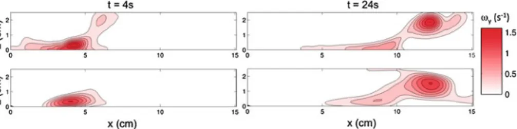
To help evaluating the impact of the scanning errors on vertical gradient computation, Fig.2shows a comparison of horizontal spanwise vorticity (ωy) in the vertical symmetry plane measured via 2D PIV and via the present 3D-3C scanning PIV technique. Top and bottom rows of Fig.2correspond to 2D PIV and 3D scanning PIV, respectively, and two different times in the evolution of the flow are shown in each column. It is important to note that the 2D and 3D measurements were performed on two distinct experiments with the same physical parameters. It can be seen that the main flow features are adequately reproduced and a good agreement is obtained between the two methods which highlight the relevance of the 3D technique. It can be seen in Fig.2that both techniques yield the same flow topology,
Fig. 2 Spanwise vorticity ωy(s−1), in the vertical symmetry plane. Comparison at two different times between
with the presence of an evolving spanwise vortex, which subsequently strengthens and lifts up. Also the peak vorticity values correspond closely. However, small quantitative variations are observed. These variations can be attributed to both the errors of reproducibility of the experimental apparatus and the techniques themselves. In particular, small changes in flow and ambient conditions might exist and regions with strong vertical gradients will probably be more largely affected by vertical errors (mentioned above) in the 3D technique. Comparisons with 2D PIV in the horizontal planes also reveal good agreement (data not shown here).
3 Time evolution of the 3D structure of a vortex dipole and its spanwise vortex
In order to investigate the evolution and deformation of the complete three-dimensional vortex dipole including the associated spanwise vortex, each vortex composing the global structure must be identified. In particular, following the vortex line corresponding to the core of each vortical structure allows the dynamics of the different entities of the complex three-dimensional hydrodynamic vortex structure to be evaluated separately and as a whole. The criterion chosen here to distinguish the vortices is the λ2-criterion. It is based on the
fact that the vorticity-induced pressure reaches a minimum in a vortex cross section. In a plane, if the pressure field exhibits a local minimum, the pressure gradient is equal to zero and the second-order derivatives of the pressure field must be positive in two orthogonal directions if lying in a vortex. In order to ensure this condition, Jeong and Hussain [13] proposed a criterion derived from the decomposition of the velocity gradient tensor∇u = D + Ω , where D and Ωare, respectively, the symmetric (deformation tensor) and anti-symmetric (rotation tensor) parts of∇u. From this decomposition, a new tensor can be defined as G = DDT− ΩΩT.G is symmetric and has real eigenvalues λ1 ≥ λ2 ≥ λ3. It can be shown that negative values
of λ2are associated with the presence of a vortex. It should be noted that the λ2-criterion,
although sometimes used with 2D PIV turbulence measurements, is only valid if applied in three dimensions (or in a symmetry plane, see [3] and therefore requires the measurements to be three-dimensional with three components.
Keeping in mind that the aim of the method is to follow the dynamics of each vortex, the λ2-criterion only isolates regions of the flow corresponding to vortices as a whole without
differentiating individual structures. On the other hand, vortex lines are not necessarily asso-ciated with vortices (i.e., vortex lines could be assoasso-ciated with shear). Therefore, both vortex lines and the λ2-criterion are used here to identify the vortex cores.
The vortices are detected by operating the three following steps: first, the λ2-criterion is
computed in the whole measurement volume on a coarse mesh and the sign of the λ2values is
used to define a mask bounding vortex regions. Second, the three-component vorticity vector is calculated and once subjected to the mask, it allows to track each individual vortex line within a vortex region. Third, if two vortex lines are close enough (within 5 mm) and have the same direction (within 10◦), they are considered as belonging to the same vortex tube
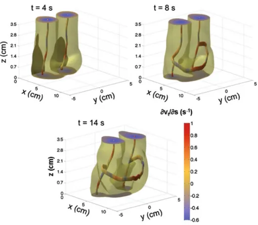
and therefore to the same vortex. They are then merged into a single vortex line. Finally, for a given vortex, the lone vortex line remaining is considered as the core vortex line. Figure3 shows an example of the resulting three-dimensional vortex lines (each vortex line being associated with a vortex), and iso-surfaces of the norm of vorticity at three different times. At t = 8 s and t = 14 s, three vortices are clearly identified: the two main vortex dipole cores and the spanwise vortex. The color along the vortex lines indicates the local value of stretching along the line ∂vt/∂s(s−1), where s and vtare the direction and the velocity vector tangent to the vortex line, respectively. It can be noted that stretching amplitude is shown here since it is suspected to have a strong influence on vortex dynamics [3].
Fig. 3 Iso-surface of the norm of vorticity ||ω0|| = (ωx2+ ωy2+ ω2z)1/2corresponding to 70 % of the maximum of its value and core vortex lines associated with the main vortex structures of the flow. The color along the vortex lines indicates the local value of stretching along the line ∂vt/∂s (s−1), where s and vtare
the direction and the velocity vector tangent to the vortex line, respectively. Snapshots of the vortex dipole are presented at t= 4, 8, and 14 s. (Re, α) = (290, 0.54)
In Fig.3, at t = 4 s, only the two almost vertical coherent vortices composing the vortex dipole are present. The vortex dipole propagating upon a solid surface develops a bound-ary layer due to the no-slip condition at the bottom. The vertical shear associated with the no-slip condition induces a bending of the vortices close to the bottom, as observed in Fig.3at t = 4 s. This shear zone is principally composed of horizontal spanwise vorticity ωy.
At t = 8 s, the λ2-criterion and vorticity line detection procedure reveal a spanwise
vortex at the front of the vortex dipole. The color on the spanwise vortex line indicates that stretching is maximal at the front of the dipole, close to the vertical plane of symmetry. This observation supports the explanation for the spanwise vortex generation proposed by Lacaze et al. [16]. They suggested that the stretching exerted by the dipole on the horizontal vorticity field associated to the developing boundary layer tends to focalize and amplify this vorticity, leading eventually to the formation of a coherent spanwise vortex. Between t= 8 s and t = 14 s, the spanwise vortex has moved upwards at the front of the primary vortex dipole. By t = 8 s, the side branches of the spanwise vortex are observed to have merged with the primary vortices composing the dipole up to the free surface. Note that the apparent orthogonal connection between the spanwise vortex and the primary vortices in Fig.3is not
physical. A better resolution is required to capture the detailed connection of the spanwise vortex legs onto the primary vortices.
4 Reconstructed pressure fields
The 3D-3C scanning PIV measurements provide an experimental evaluation of all the terms of the Navier–Stokes equation except the pressure gradient which can be deduced. The pressure field, however, is not easily obtained by direct integration of the pressure gradient in the Navier–Stokes equations because of unknown constants of integration depending on two spatial directions. This problem can be avoided by solving a Poisson equation for the pressure. The Laplacian of the pressure is computed by considering the divergence of the Navier–Stokes equations. Due to the incompressibility of the flow, the Laplacian of the pressure can be written as
∇2 P = − ∇.((u.∇)u) = S (x, y, z) ,
where P is the pressure, u is the velocity vector,∇ is the gradient operator, ∇. is the divergence operator and∇2 is the Laplacian operator. This equation is solved by a Fourier spectral
method. Based on the error estimation of the vertical velocity gradient given in Sect.2.3, the product of velocity gradients needed here to evaluate the pressure field yields errors less than 15 %.
The top row in Fig.4shows cross-sectional distributions of∇2P (in color) extracted
from the 3D-3C scanning PIV measurements of a vortex dipole for (Re, α) = (290, 0.54) at
t = 4, 8, 14 and 22s in the horizontal plane z = h/3 and the vertical plane of symmetry
y= 0. The black contours are iso-contours of the vorticity perpendicular to the measurement plane (namely ωz in the horizontal plane and ωyin the vertical one). It should be recalled that a vortex can be identified by a sectional minimum of the pressure P, which is equivalent to a maximum of the Laplacian of the pressure∇2P.
In the top row of Fig.4, according to the pressure criterion, only the primary vortices composing the vortex dipole are observed at t= 4 s. At t = 8 s, the boundary layer generated by the vortex dipole propagation over the solid bottom has become slightly thicker. In the vertical symmetry plane, a positive∇2Pis observed in the upper part of the boundary layer
and its altitude corresponds to the location of the spanwise vortex given by the λ2-criterion
in Fig.3at t = 8 s. At t = 14 s in the vertical plane of symmetry, the black contours of the spanwise vorticity indicate that a spanwise vortex has detached from the boundary layer vorticity. The core of the spanwise vortex is clearly marked by a maximum of∇2P. At
t= 14 s the altitude of the spanwise vortex is approximately z = h/3, it is then slightly above this horizontal plane at t = 22 s. The secondary spanwise vortex is accordingly detected in the horizontal plane z = h/3 at the front of the primary vortices through its signature by a local maximum of∇2P.
The ability of the flow to put sediments into suspension can be estimated through the strength of the vertical pressure gradient. Slices of the vertical pressure gradient in the hori-zontal plane z= h/3 and the vertical plane of symmetry y = 0 are shown in the bottom row of Fig.4at t= 4, 8, 14 and 22s.
At t = 4 s in the horizontal plane, the vertical pressure gradient is negative between the two primary vortices and positive at the front and at the rear of the vortex dipole. In the horizontal plane, along the streamwise direction, this quasi-rear-front symmetry of the vertical pressure gradient (positive on each side) is an additional evidence of the initial quasi
Fig .4 Laplacian of the pressure ∇ 2P (P a m − 2) (top row ) and vertical pressure gradient ∂ P / ∂ z (P a m − 1) (bottom row )i nt he horizontal plane (x, y) at z = h / 3a nd th e vertical plane (x ,z ) of symmetry of the dipole y = 0 (in color ). The blac k contour s are iso-contours of the vorticity perpendicular to the plane considered (namely ωz in the horizontal plane and ωy in the vertical one). From left to right ,s napshots of the vorte x dipole are presented at t= 4, 8, 14 and 22 s, respecti vely .( Re , α ) = (290 , 0. 54 )
two-dimensionality of the vortex dipole. At t = 8 s, the positive vertical pressure gradient becomes predominant at the front of the dipole. The negative vertical pressure gradient is mainly located between the two primary vortices and slightly extends in the vertical plane of symmetry ahead of the primary vortices centroids. This feature is even more noticeable at
t= 14 and 22s. Moreover, the streamwise position of the negative vertical pressure gradient is located just between the streamwise position of the primary vortices (black contours in the horizontal plane) and the streamwise position of the spanwise vortex (black contours in the vertical plane of symmetry). The likely upwelling associated to the negative vertical pressure gradient is then expected to take place ahead of the vortex dipole and at the rear of the spanwise vortex.
5 Reconstructed wall shear stress and skin friction lines
Many studies have shown that vortex dipoles could play an important role in mass transport. More precisely in shallow water coastal zones, vortex dipoles are responsible for sand bed deformation [15,19,21] or suspension of sediments from the seabed [1]. Yet our physical understanding of the creeping, saltation or suspension processes of bed load is still incomplete. In that context, the 3D-3C scanning PIV measurements of the present study give valuable information since they allow the influence of the flow generated by the vortex dipole to be quantified by computing the complete (x, y) shear stress on the bottom surface. If the dipole propagates above a sediment bed, its induced wall shear stress may mobilize sediment and transport it downstream, either as bed load or suspended load if strong enough.
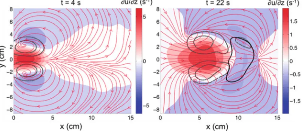
The wall shear stress is shown in Fig.5in the form of skin friction lines, or streamlines of the wall shear stress vector (∂u/∂z, ∂v/∂z), where u and v are the streamwise and spanwise horizontal velocity components, respectively. The scalar streamwise shear stress ∂u/∂z is also displayed in color.
In Fig.5, at t = 4 s, the topology of the friction lines is typical of a vortex dipole. The pair of counter-rotating vortices is associated with two convergent or attractive foci,
Fig. 5 Streamwise wall shear stress ∂u/∂z(s−1)in the horizontal plane (x, y) at z= 0 (in color). The grey
dashed contoursand black solid contours are iso-contours of vertical vorticity ωzand spanwise vorticity ωy
at z= h/3 and indicate the position of the vortex dipole and the spanwise vortex, respectively. The red lines show the skin friction lines associated with wall shear stress (∂u/∂z, ∂v/∂z) in the horizontal plane (x, y) at
z= 0. From left to right, snapshots of the vortex dipole are presented at t = 4 and 22 s, respectively. (Re, α) =
which are evidence of a vertical fluid motion in the core of both vortices [7]. Moreover, the wall boundary conditions at the bottom impose this fluid motion to be upwards. This upwelling flow is expected to favor sediment suspension from the bottom bed into the vortex cores. At this early stage of development, the flow is also characterized by the presence of a region of strong positive streamwise wall shear stress between the vortices. If the shear stress is strong enough, this part of the flow is expected to dominate the downstream sediment entrainment. Moreover extrema of negative shear stress are observed on the sides of the vortex pair, which could lead to upstream sediment transport laterally. The global topology of the friction lines suggests that the propagation of the dipole could erode the sediment bed along its trajectory.
In Fig.5, at t = 22 s, the wall shear stress and the topology of the skin friction lines under the primary vortices of the dipole are qualitatively the same. But the generation of the spanwise vortex leads to a radically different situation in the front of the dipole compared to t = 4 s. More precisely, the velocity induced by the spanwise vortex produces a large region of negative streamwise shear stress in the vicinity of the y = 0 axis, with friction lines in front of the dipole directed upstream, just below the spanwise vortex. This feature is associated with the joint creation of an attachment node downstream of the spanwise vortex (at x ≈ 12 cm), and a detachment node just upstream (at x ≈ 9 cm). This adverse shear stress is expected to sweep the bed load back, in opposite direction than the positive shear stress induced upstream between the primary vortices of the dipole, which transports sediments forward. The combination of these two mechanisms could lead to an efficient bed load transport towards the detachment node, where the sediments could be put into suspension by the associated upward flow at that point. It is noteworthy that such a flow structure is very similar to the design of carpet sweepers, with two main brushes counter-revolving round a vertical axis, and a third brush spinning round a horizontal axis at the front. Such a mechanical device proves to be particularly efficient to clean dust and crumbs up from the floor. We conjecture that its hydrodynamic equivalent could be as efficient to transport and put sediment into suspension.
6 Conclusion
In the last decade numerous studies have addressed the effect of shallowness on the quasi two-dimensionalization of flows. In particular the generation of vortex dipoles, that are recur-rent hydrodynamic structures in geophysical flows, well known for their ability to transport mass over large distances, have been the subject of several studies [17,22,23]. Even though shallowness seems to reduce vertical motions a three-dimensional spanwise vortex has often been observed at the front of shallow dipolar vortices [2,3,8,16,22,23]. The conditions under which such a secondary structure develops has been investigated by means of numerical sim-ulations and classical 2D PIV measurements by Duran-Matute et al. [8] and Albagnac et al. [3]. A physical mechanism for the generation and maturation of the spanwise vortex has been proposed by Lacaze et al. [16]. Nevertheless, one needs to access three-dimensional dynamics to complete our understanding on spanwise vortex generation process, its topology, its time evolution and interaction with the primary dipolar structure. To this end, a 3D-3C scanning PIV technique has been developed to obtain the full three-dimensional structure of shallow vortex dipoles and the associated spanwise vortex. In particular, measurements in a volume of the three velocity components and their gradients, resolved in time, provide access to all the terms of the Navier–Stokes equation, including the pressure field and its gradient. The overall findings of the present study are in agreement with those of Sous et al. [22,23],
Akkermans et al. [2], Lacaze et al. [16], Duran-Matute et al. [8] and Albagnac et al. [3] but some new aspects have been found and are resumed hereafter.
The present study confirms that the stretching field, which contributes to the generation of the spanwise vortex, reaches a maximum of intensity in the vertical symmetry plane at the front of the dipole. This location corresponds to the zone where the spanwise vortex is observed in its premature stage (see Fig.3). This confirms the role of the stretching field induced by the vortex dipole, in the generation and dynamics of the spanwise vortex [16].
Regarding the topology of the secondary vortical structure, the side branches of the span-wise vortex are tracked in three dimensions with a vortex recognition algorithm based on the λ2-criterion and the vorticity vector. These branches are observed to bend downstream
and incline upwards before connecting with the primary vortices composing the vortex dipole.
This complex structure has implications for the possible mechanisms responsible for mass transport associated with shallow vortex dipoles observed in geophysical applications. To investigate these more closely, the pressure field and its derivatives were also computed. It is shown that the vertical pressure gradient is negative and exhibits a minimum at the front of the vortex dipole and at the rear of the spanwise vortex. This is confirmed by the analysis of the skin friction lines associated to the wall shear stress, which exhibit a detachment node at the same location. The resulting 3D flow structure and inferred mass transport can therefore be considered as the hydrodynamic equivalent of a mechanical carpet sweeper.
Future work includes further experiments in the presence of a bed of particles at the bottom of the tank in order to qualify and quantify the effect of the vortex dipole with or without spanwise vortex (depending on the value of α2Re) on the transport of sediments. The
three-dimensional experimental data will also be used as an initial condition into a numerical code to investigate the Lagrangian transport of particles.
Acknowledgments The authors would like to thank N. Boulanger, S. Cazin, E. Cid, A. Fincham, H. Merzisen
and A. Paci for their help in the development of the 3D-3C scanning PIV technique. J. Albagnac acknowledges financial support from the French Government MENRT in the form of a graduate scholarship. Funding by the University Paul Sabatier’s BQR program is also acknowledged.
References
1. Ahlnas K, Royer T, George T (1987) Multiple dipole eddies in the Alaska coastal current detected with Landsat thematic mapper data. J Geophys Res 92:13041–13047
2. Akkermans R, Cieslik A, Kamp L, Clercx H, Van Heijst G (2008) The three-dimensional structure of an electromagnetically generated dipolar vortex in a shallow fluid layer. Phys Fluid 554(20):116601 3. Albagnac J, Lacaze L, Brancher P, Eiff O (2011) On the existence and evolution of a spanwise vortex in
laminar shallow water dipoles. Phys Fluid 23:086601
4. Billant P, Chomaz JM (2000) Experimental evidence for a new instability of a vertical columnar vortex pair in a strongly stratified fluid. J Fluid Mech 418:167–188
5. Boulanger N, Eiff O, Paci A, Fincham A, Moulin FM (2013) A novel scanning correlation imaging velocimetry (SCIV) technique applied to turbulent lee-wave breaking. Exp Fluid (To be submitted) 6. Chen Q, Dalrymple RA, Kirby JT, Kennedy AB, Haller MC (1999) Boussinesq modeling of a rip current
system. J Geophys Res 104(C9):20617–20637
7. Délery JM (2001) Robert Legendre and Henri Werlé: toward the elucidation of three-dimensional sepa-ration. Annu Rev Fluid Mech 33:129–154
8. Duran-Matute M, Albagnac J, Kamp L, Van Heijst G (2010) Dynamics and structure of decaying shallow dipolar vortices. Phys Fluid 22:116606
9. Elsinga GE, Scarano F, Wieneke B, van Oudheusden BW (2006) Tomographic particle image velocimetry. Exp Fluid 41:933–947
10. Fincham AM, Spedding GR (1997) Low cost, high resolution DPIV for measurement of turbulent fluid flow. Exp Fluid 23(6):449–462
11. Fincham A (2003) 3 component, volumetric, time-resolved scanning correlation imaging velocimetry. In: Proceedings of 5th international symposium on particle image velocimetry, Busan, Korea, pp 2–16 12. Fincham AM (2006) Continuous scanning, laser imaging velocimetry. J Vis 9(3):247–255
13. Jeong J, Hussain F (1995) On the identification of a vortex. J Fluid Mech 285:69–94
14. Jirka G (2001) Large scale flow structures and mixing processes in shallow flows. J Hydraul Res 39:567– 573
15. Johnson D, Pattiaratchi C (2006) Boussinesq modeling of transient rip currents. Coast Eng 53:419–439 16. Lacaze L, Brancher P, Eiff O, Labat L (2010) Experimental characterization of the 3D dynamics of a
laminar shallow vortex dipole. Exp Fluid 48(2):225–231
17. Lin J, Ozgoren M, Rockwell D (2003) Space-time development of the onset of a shallow-water vortex. J Fluid Mech 485:33–66
18. Peregrine DH (1998) Surf zone currents. Theor Comput Fluid Dyn 10:295–309
19. Reniers A, Roelvink J, Thornton E (2004) Morphodynamic modeling of an embayed beach under wave group forcing. J Geophys Res 109:C01030
20. Rockwell D, Lin JC, Fu H, Orgozen M (2003) Vortex formation in shallow Flows. In: International Symposium on shallow flows
21. Smith J, Largier J (1995) Observations of nearshore circulations: rip currents. J Geophys Res 100:10967– 10975
22. Sous D, Bonneton N, Sommeria J (2004) Turbulent vortex dipoles in a shallow water layer. Phys Fluid 16(8):2886–2898
23. Sous D, Bonneton N, Sommeria J (2005) Transition from deep to shallow water layer: formation of vortex dipoles. Eur J Mech B Fluid 24:19–32
24. Tew Kai E, Rossi V, Sudre J, Weimerskirch H, Lopez C, Hernandez-Garcia E, Marsac F, Garcon V (2009) Top marine predators track Lagrangian coherent structures. PNAS 106(20):8245–8250
25. Uijtewaal WSJ, Booij R (2000) Effects of shallowness on the development of free-surface mixing layers. Phys Fluid 12(2):394–402