HAL Id: hal-02613135
https://hal.archives-ouvertes.fr/hal-02613135v3
Preprint submitted on 27 Mar 2021
HAL is a multi-disciplinary open access
archive for the deposit and dissemination of sci-entific research documents, whether they are pub-lished or not. The documents may come from teaching and research institutions in France or
L’archive ouverte pluridisciplinaire HAL, est destinée au dépôt et à la diffusion de documents scientifiques de niveau recherche, publiés ou non, émanant des établissements d’enseignement et de recherche français ou étrangers, des laboratoires
A Weissman-type estimator of the conditional marginal
expected shortfall
Yuri Goegebeur, Armelle Guillou, Nguyen Khanh Le Ho, Jing Qin
To cite this version:
Yuri Goegebeur, Armelle Guillou, Nguyen Khanh Le Ho, Jing Qin. A Weissman-type estimator of the conditional marginal expected shortfall. 2021. �hal-02613135v3�
A Weissman-type estimator of the conditional marginal expected
shortfall
Yuri Goegebeurp1q, Armelle Guilloup2q, Nguyen Khanh Le Hop1q, Jing Qinp1q
p1q Department of Mathematics and Computer Science, University of Southern
Denmark, Campusvej 55, 5230 Odense M, Denmark
p2q Institut Recherche Math´ematique Avanc´ee, UMR 7501, Universit´e de Strasbourg et
CNRS, 7 rue Ren´e Descartes, 67084 Strasbourg cedex, France
Abstract
The marginal expected shortfall is an important risk measure in finance and actuarial science, which has been extended recently to the case where the random variables of main interest are observed together with a covariate. This leads to the concept of conditional marginal expected shortfall for which an estimator is proposed allowing extrapolation out-side the data range. The main asymptotic properties of this estimator have been established, using empirical processes arguments combined with the multivariate extreme value theory. The finite sample behavior of the proposed estimator is evaluated with a simulation experi-ment, and the practical applicability is illustrated on vehicle insurance customer data. Keywords: Conditional marginal expected shortfall, extrapolation, Pareto-type distribu-tion.
1
Introduction
A central topic in actuarial science and finance is the quantification of the risk of a loss variable. This is done by risk measures, the most basic among them is the Value-at-Risk (VaR), defined as the p´quantile of a loss variable Y :
Qppq :“ infty : FYpyq ě pu, p P p0, 1q,
where FY denotes the distribution function of Y . We refer to Jorion (2007) for a review. The
main drawbacks of VaR are that it does not take the loss above this p´quantile into consideration and it is not a coherent risk measure (Artzner et al., 1999). Recently, the conditional tail expectation (CTE), defined as
Artzner et al (1999), Cai and Tan (2007) and Brazaukas et al. (2008). The conditional tail expectation has also been extended to the multivariate context, leading to the concept of the marginal expected shortfall (MES). For a pair of risk factors pYp1q, Yp2q
q, the marginal expected shortfall is defined as
θp “ EpYp1q|Yp2q ą Q2p1 ´ pqq, p P p0, 1q,
where Q2 denotes the quantile function of risk factor Yp2q. This measure was introduced by
Archarya et al. (2010), to measure the contribution of a financial firm to an overall systemic risk. For a financial firm, the MES is defined as its short-run expected equity loss conditional on the market taking a loss greater than its VaR. Cai et al. (2015) studied the MES in a bivariate extreme value framework, and proposed an estimator for it when the Yp2q quantile is extreme,
i.e., when p ă 1{n, where n is the sample size, leading to extrapolations outside the data range. We also refer to Landsman and Valdez (2003), Cai and Li (2005), Barg`es et al. (2009), Cousin and Di Bernardino (2013), Di Bernardino and Prieur (2018), Das and Fasen-Hartmann (2018, 2019).
Recently, Goegebeur et al. (2020) have considered the estimation of the marginal expected shortfall, but this time in case where the random variables of main interest pYp1q, Yp2qq are
recorded together with a random covariate X P Rd. This leads to the concept of conditional marginal expected shortfall, given X “ x0, and defined as
θppx0q “ E ” Yp1q ˇ ˇ ˇY p2q ě QYp2q ´ 1 ´ p ˇ ˇ ˇx0 ¯ ; X “ x0 ı .
In the sequel, we will denote by Fjp¨|xq the continuous conditional distribution function of
Ypjq, j “ 1, 2, given X “ x, and use the notation F
jp¨|xq for the conditional survival function
and Ujp¨|xq for the associated tail quantile function defined as Ujp¨|xq “ infty : Fjpy|xq ě 1´1{¨u.
Also, we will define by fX the density function of the covariate X and by x0a reference position
such that x0 P IntpSXq, the interior of the support SX Ă Rd of fX, which is assumed to
be non-empty. Considering pYip1q, Yip2q, Xiq, i “ 1, . . . , n, independent copies of pYp1q, Yp2q, Xq,
Goegebeur et al. (2020) proposed the following nonparametric estimator for θk{npx0q
θk npx0q :“ 1 k řn i“1Khnpx0´ XiqY p1q i 1ltYip2qě pU2pn{k|x0qu p fnpx0q , where Khnp.q :“ Kp.{hnq{h d
n, with K a joint density function on Rd, k an intermediate sequence
such that k Ñ 8 with k{n Ñ 0, hna positive non-random sequence of bandwidths with hnÑ 0
if n Ñ 8, 1lA the indicator function on the event A, and pfnpx0q :“ p1{nq
řn
i“1Khnpx0´ Xiq
is a classical kernel density estimator. Here, pU2p.|x0q is an estimator for U2p.|x0q, defined as
p
U2p.|x0q :“ infty : pFn,2py|x0q ě 1 ´ 1{.u where
p Fn,2py|x0q :“ 1 n řn i“1Khnpx0´ Xiq1ltYp2q i ďyu p fnpx0q . (1)
The asymptotic behavior of θk{npx0q has been established by Goegebeur et al. (2020) and is
recalled in Theorem 5.1 in Section 5. Due to the conditions k, n Ñ 8 with k{n Ñ 0, the Yp2q-quantile is intermediate, and thus the estimator θ
k{npx0q cannot be used for extrapolation
outside the Yp2q-data range. Extrapolation is relevant for practical data analysis, since often
we want to go beyond the range of the available data. With a classical empirical estimator like θppx0q where p ă 1{n this is not possible, as it would always lead to the trivial estimate of
zero. The aim of this paper is to solve this issue and to define a new estimator which allows extrapolation and thus which is valid for p ă 1{n.
The Value-at-Risk and conditional tail expectation mentioned above have also been studied in an extreme value framework with random covariates. As for the estimation of extreme condi-tional quantiles we refer to Daouia et al. (2011, 2013). In El Methni et al. (2014), for the framework of heavy-tailed distributions, the conditional tail expectation was generalised to the conditional tail moment, and estimators were introduced for the situation where the variable of main interest Y was observed together with a random covariate X. This work was extended to the general max-domain of attraction in El Methni et al. (2018).
The remainder of the paper is organized as follows. In Section 2, we introduce our estimator for the conditional marginal expected shortfall allowing extrapolation and we establish its main asymptotic properties. The efficiency of our estimator is examined with a small simulation study in Section 3. Finally, in Section 4 we illustrate the performance of our estimator on vehicle insurance customer data. Some preliminary results are given in Section 5, whereas the proofs of the main results are postponed to Section 6.
2
Estimator and asymptotic properties
We assume that Yp1q and Yp2q are positive random variables, and that they follow a conditional
Pareto-type model. Let RVψ denote the class of regularly varying functions at infinity with
index ψ, i.e., positive measurable functions f satisfying f ptxq{f ptq Ñ xψ, as t Ñ 8, for all x ą 0. If ψ “ 0, then we call f a slowly varying function at infinity.
Assumption pDq For all x P SX, the conditional survival function of Ypjq, j “ 1, 2, given
X “ x, satisfies Fjpy|xq “ Ajpxqy´1{γjpxq ˆ 1 ` 1 γjpxq δjpy|xq ˙ ,
where Ajpxq ą 0, γjpxq ą 0, and |δjp.|xq| is normalized regularly varying at infinity with index
´βjpxq, βjpxq ą 0, i.e., δjpy|xq “ Bjpxq exp ˆży 1 εjpu|xq u du ˙ ,
Clearly, Assumption pDq implies that Ujp¨|xq, j “ 1, 2, satisfy
Ujpy|xq “ rAjpxqsγjpxqyγjpxqp1 ` ajpy|xqq , (2)
where ajpy|xq “ δjpUjpy|xq|xqp1 ` op1qq, and thus |ajp.|xq| P RV´βjpxqγjpxq.
Now, to estimate θppx0q it is required to impose an assumption on the right-hand upper tail
dependence of pYp1q, Yp2qq, conditional on a value of the covariate X. Let R
tpy1, y2|xq :“
tPpF1pYp1q|xq ď y1{t, F2pYp2q|xq ď y2{t|X “ xq.
Assumption pRq For all x P SX we have as t Ñ 8
Rtpy1, y2|xq Ñ Rpy1, y2|xq,
uniformly in y1, y2 P p0, T s, for any T ą 0, and in x P Bpx0, rq, for any r ą 0.
Assuming pDq with γ1px0q ă 1 and pRq, one can show (see Cai et al., 2015, Proposition 1) that
lim pÑ0 θppx0q U1p1{p|x0q “ ´ ż8 0 Rps, 1|x0qds´γ1px0q,
from which the following approximation can be deduced θppx0q „ U1p1{p|x0q U1pn{k|x0q θk npx0q „ ˆ k np ˙γ1px0q θk npx0q.
Thus, to estimate θppx0q, we need first to estimate γ1px0q. We propose the following estimator
p γ1,k1px0q :“ 1 k1 řn i“1Khnpx0´ Xiq ´ ln Yip1q´ ln pU1pn{k1|x0q ¯ 1l tYip1qě pU1pn{k1|x0qu p fnpx0q , (3)
based on an intermediate sequence k1 such that k1Ñ 8 with k1{n Ñ 0. This sequence may be
different from k, the one used in the estimator θk
npx0q, but the two sequences are linked together
(see Theorem 2.2 below). On the contrary, for convenience, we use the same bandwidth hn and
kernel K for both the estimation of γ1px0q and θppx0q. Note thatpγ1,k1px0q is a local version of
the Hill estimator (Hill, 1975) from the univariate extreme value context. Now, we are able to define a Weissman-type estimator for θppx0q, given by
p θppx0q “ ˆ k np ˙pγ1,k1px0q θk npx0q.
Our aim in this paper is to establish the asymptotic behavior of pθppx0q, which requires the
asymp-totic behavior ofpγ1,k1px0q in terms of the process on which the estimator θk
npx0q is based on (see
Theorem 5.1 in Section 5). To reach this goal, some assumptions due to the regression context are required. In particular, fXp.q, Rpy1, y2|.q and the functions appearing in Fjpy|.q, j “ 1, 2,
are assumed to satisfy the following H¨older conditions. Let }.} denote some norm on Rd. Assumption pHq There exist positive constants MfX, MR, MAj, Mγj, MBj, Mεj, ηfX, ηR,
ηAj, ηγj, ηBj, ηεj, where j “ 1, 2, and β ą γ1px0q, such that for all x, z P SX:
|fXpxq ´ fXpzq| ď MfX}x ´ z} ηfX, sup y1ą0,12ďy2ď2 |Rpy1, y2|xq ´ Rpy1, y2|zq| yβ1 ^ 1 ď MR}x ´ z}ηR, |Ajpxq ´ Ajpzq| ď MAj}x ´ z} ηAj , |γjpxq ´ γjpzq| ď Mγj}x ´ z} ηγj , |Bjpxq ´ Bjpzq| ď MBj}x ´ z} ηBj , and sup yě1 |εjpy|xq ´ εjpy|zq| ď Mεj}x ´ z} ηεj .
We also impose a condition on the kernel function K, which is a standard condition in local estimation.
Assumption pKq K is a bounded density function on Rd, with support SK included in the unit
ball in Rd, with respect to the norm }.}.
Our first aim, now, is to show the weak convergence, denoted , of the process based on p
γ1,k1px0q, but in terms of the same process as the one used in Theorem 2.3 from Goegebeur et
al. (2020).
Theorem 2.1 Assume pDq, pHq, pKq, x0 P IntpSXq with fXpx0q ą 0, and y Ñ F1py|x0q,
is strictly increasing. Consider sequences k1 Ñ 8 and hn Ñ 0 as n Ñ 8, in such a way
that k1{n Ñ 0, k1hdn Ñ 8, h ηε1 n ln n{k1 Ñ 0, a k1hdnh ηfX^ηA1 n Ñ 0, a k1hdnh ηγ1 n ln n{k1 Ñ 0, a k1hdn|δ1pU1pn{k1|x0q|x0q| Ñ 0. Then we have, b k1hdnppγ1,k1px0q ´ γ1px0qq γ1px0q fXpx0q „ż1 0 W pz, 8q1 zdz ´ W p1, 8q , where W pz, 8q is a zero centered Gaussian process with covariance function
EpW pz, 8qW pz, 8qq “ }K}22fXpx0q pz ^ zq , with }K}2 :“ b ş RdK 2puqdu.
Before stating the weak convergence of pθppx0q, we need to introduce a second order condition,
usual in the extreme value context.
Assumption pSq. There exist β ą γ1px0q and τ ă 0 such that, as t Ñ 8
sup xPBpx0,rq sup y1ą0,12ďy2ď2 |Rtpy1, y2|xq ´ Rpy1, y2|xq| yβ1 ^ 1 “ Opt τ q, for any r ą 0.
Our final result is now the following.
Theorem 2.2 Assume pDq, pHq, pKq, pSq with x Ñ Rpy1, y2|xq being a continuous function,
and y Ñ Fjpy|x0q, j “ 1, 2, are strictly increasing. Let x0 P IntpSXq such that fXpx0q ą 0.
Consider sequences k “ tnα`1pnqu, k1 “ tnα1`2pnqu and hn“ n´∆`3pnq, where `1, `2 and `3 are
slowly varying functions at infinity, with α P p0, 1q and α ď α1 ă min ˆ α drd ` 2 pηfX^ ηA1 ^ ηγ1qs , α ` 2γ1px0qβ1px0q 1 ` 2γ1px0qβ1px0q ˙ , and max ˆ α d ` 2γ1px0qpηR^ ηA1^ ηγ1q , α d ` 2p1 ´ γ1px0qqpηA2^ ηγ2^ ηB2 ^ ηε2 ^ ηfXq , α d´ 2p1 ´ αqγ12px0qβ1px0q d ` dpβ1px0q ` εqγ1px0q ,α ´ 2p1 ´ αqpγ1px0q ^ pβ2px0qγ2px0qq ^ p´τ qq d , α1 d ` 2 pηfX^ ηA1 ^ ηγ1q ,α1´ 2p1 ´ α1qγ1px0qβ1px0q d ¯ ă ∆ ă α d. Then, for γ1px0q ă 1{2 and p satisfying p ď kn such that ln k{pnpq?
k1hdn Ñ 0 and b k k1 ln k np Ñ r P r0, 8s, we have min ˜ b khd n, a k1hdn ln k{pnpq ¸ ˜ p θppx0q θppx0q ´ 1 ¸ minpr, 1qγ1px0q fXpx0q ˆż1 0 W py, 8q1 ydy ´ W p1, 8q ˙ ` min ˆ 1,1 r ˙# ´p1 ´ γ1px0qq W p8, 1q fXpx0q ` 1 fXpx0q ş8 0 W py, 1qdy ´γ1px0q ş8 0 Rpy, 1|x0qdy´γ1px0q + , where W py1, y2q is a zero centered Gaussian process with covariance function
E pW py1, y2qW py1, y2qq “ }K}22fXpx0qRpy1^ y1, y2^ y2|x0q,
W py, 8q is the limiting process of Theorem 2.1, and W p8, yq is a zero centered Gaussian process with covariance function
The variance of the limiting random variable in Theorem 2.2, denoted W, is given by VarpWq “ }K} 2 2 fXpx0q # pminpr, 1qq2γ12px0q ` ˆ min ˆ 1,1 r ˙˙2„ γ12px0q ´ 1 ´ c2 ż8 0 Rps, 1|x0qds´2γ1px0q `2 min ˆ r,1 r ˙ γ1px0q « p1 ´ γ1px0q ` cq Rp1, 1|x0q ´ ż1 0 ´ 1 ´ γ1px0q ` cs´γ1px0qp1 ´ γ1px0q ´ γ1px0q ln sq ¯Rps, 1|x 0q s ds ff+ , (4) where c :“ pş08Rps, 1|x0qds´γ1px0qq´1.
3
Simulation experiment
In this section, we illustrate the finite-sample performance of our conditional marginal expected shortfall estimator with a simulation experiment. To this aim, we consider the three models already used in Goegebeur et al. (2020), but this time in the case where p ă 1{n, i.e., allowing extrapolation outside the Yp2q´data range. These models are the following:
Model 1: The conditional logistic copula model, defined as Cpu1, u2|xq “ e´rp´ ln u1q
x`p´ ln u
2qxs1{x, u
1, u2P r0, 1s, x ě 2. (5)
In this model, X is uniformly distributed on the interval r2, 10s, and the marginal distribution functions of Yp1q and Yp2q are Fr´echet distributions:
Fjpyq “ e´y ´1{γj
, y ą 0,
j “ 1, 2. We set γ1 “ 0.25 and γ2 “ 0.5. It can be shown that this model satisfies Assumption
pSq with Rpy1, y2|xq “ y1` y2´ pyx1 ` y2xq1{x, τ “ ´1 and β “ 1 ´ ε for some small ε ą 0.
Model 2: The conditional distribution of pYp1q, Yp2qq given X “ x is that of
p|Z1|γ1pxq, |Z2|γ2pxqq,
where pZ1, Z2q follow a bivariate standard Cauchy distribution with density function
f pz1, z2q “
1 2πp1 ` z
2
1 ` z22q´3{2, pz1, z2q P R2.
Again, Assumption pSq is satisfied for this model with Rpy1, y2|xq “ y1` y2´
a y2
1` y22, τ “ ´1
and β “ 2 (see, e.g., Cai et al., 2015, in the context without covariates).
Model 3: We consider again the conditional logistic copula model defined in (5) but this time with conditional Burr distributions for the marginal distribution functions of Yp1q and Yp2q, i.e.,
Fjpy|xq “ 1 ´ ˆ βj βj ` yτjpxq ˙λj , y ą 0; βj, λj, τjpxq ą 0, j “ 1, 2. We set β1 “ β2 “ 1, λ1“ 1, λ2 “ 0.5, and τ1pxq “ 2e0.2x, τ2pxq “ 8{ sinp0.3xq.
Similarly to Model 1, this model satisfies pSq.
Note that for all these models, Assumption pDq is satisfied since all the marginal conditional distributions are standard examples from this class of heavy-tailed distributions (see, e.g., Beir-lant et al., 2009, Table 1), and Assumption pHq also holds.
We simulate 500 datasets of size n “ 500 and 1 000 from each model. For each sample, we compute pθppx0q for two different values of p: 1{p2nq and 1{p5nq, and three different sets of
val-ues of the covariate position x0: t3, 5, 7u for Model 1 and Model 3, and t0.3, 0.5, 0.8u for Model 2.
Concerning the kernel function K, we use the bi-quadratic function Kpxq “ 15
16p1 ´ x
2
q21ltxPr´1,1su,
for both the estimation ofpγ1,k1px0q and θk{npx0q. This kernel function clearly satisfies
Assump-tion pKq. To compute these estimators, we need also to select a bandwidth hn. To this aim, we
use the cross-validation procedure introduced by Yao (1999), and already used in the extreme value framework by Daouia et al. (2011, 2013) and Escobar-Bach et al. (2018a), and defined as:
hcv :“ argmin hnPH n ÿ i“1 n ÿ j“1 ˆ 1l! Yip2qďYj2q )´ pFn,h n,2,´i ´ Yjp2q ˇ ˇ ˇXi ¯˙2 , (6)
where H is the grid of values defined as RX ˆ t0.05, 0.10, . . . , 0.30u, with RX the range of the
covariate X, and p Fn,hn,2,´ipy|xq :“ řn k“1,k‰iKhnpx ´ Xkq 1l!Yp2q k ďy ) řn k“1,k‰iKhnpx ´ Xkq .
Concerning the choice of the sequence k1 in the estimation of γ1px0q, a graphical assessment is
used. The retained value of k1 corresponds to the smallest value of k after which the median of
extreme value theory where we search at a plateau of an extreme value estimator as a function of the intermediate sequence.
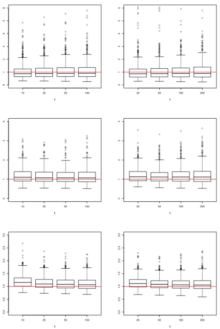
Figures 1 to 6 display the boxplots of the ratios between the estimates pθppx0q and the true value
θppx0q based on the 500 replications for the different values of x0 (corresponding to the rows)
and the two sample sizes (corresponding to the columns: n “ 500 on the left, n “ 1 000 on the right). Figures 1 and 2 correspond to Model 1 for p “ 1{p2nq and 1{p5nq, respectively. Similarly, Figures 3 and 4 correspond to Model 2, and Figures 5 and 6 to Model 3.
Based on these simulations, we can draw the following conclusions:
• Our estimator pθppx0q performs quite well in all the situations, although its efficiency
de-pends obviously on the model and also on the covariate position. This is expected because as is clear from our models, the marginal distributions in Model 1 do not depend on the covariates but the dependence structure does. On the contrary, the dependence structure in Model 2 does not depend on the covariate but the marginal distributions depend on x0,
and in Model 3 both of them depend on x0. Thus, Model 1 is less challenging than the
two other models;
• Note that the estimation in Model 2 is difficult and depends a lot on the value of the covariate. This can be explained by the fact that the plot of γ1pxq as a function of x
exhibits two local maxima, one of which being close to 0.3, and a local minimum at 0.5. Thus, we get an underestimation of θppx0q near the local maxima and an overestimation
of θppx0q near the local minima, due to the local nature of the estimation. Outside these
neighborhoods, the estimation is without bias. This is the case for x0 “ 0.8. Note also
that sometimes a local bandwidth instead of a global one as in (6) can give better results, especially at covariate positions where the function γ1pxq changes quickly;
• As expected, the smaller p is, the more difficult is the estimation, due to an important extrapolation outside the Yp2q
´data range. This results in an increase of the variability of the estimates. Note that the values p “ 1{p2nq and p “ 1{p5nq correspond to quite severe extrapolations since the estimation is done locally, and the local number of observations is much smaller than n.
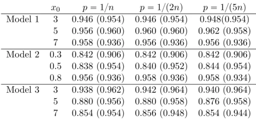
Next, we investigate in Table 1 the coverage probabilities of the pointwise 95% confidence inter-vals for θppx0q, based on a log-scale version of Theorem 2.2, namely for
min ˜ b khd n, a k1hdn ln k{pnpq ¸ lnθpppx0q θppx0q ,
which has the same limiting distribution as in Theorem 2.2, and this for the three models with their different values of x0, and three values for p: 1{n, 1{p2nq and 1{p5nq. These confidence
intervals are given by » — — — — – p θppx0q exp # Φ´1`1 ´α 2 ˘ b { VarpWq an + , p θppx0q exp # ´Φ´1`1 ´ α2˘ b { VarpWq an + fi ffi ffi ffi ffi fl , (7) where an:“ minp a khd n, a
k1hdn{pln k{pnpqq, Φ´1denotes the standard normal quantile function
andVarpWq is an estimate for the asymptotic variance given in (4), obtained by using the local{ Hill estimate (3) for γ1px0q and the following estimate for Rpy1, y2|x0q:
p Rpy1, y2|x0q “ 1 k řn i“1Khnpx0´ Xiq 1l!Fp n,1pYip1q|Xiqďnky1, pFn,2pYip2q|Xiqďkny2 ) p fnpx0q , (8)
where pFn,1 is a kernel estimator for F1, of the same form as pFn,2 given in (1). Note that this
estimator (8) can be viewed as an adjusted version of the estimator proposed in the context of estimation of the conditional stable tail dependence function by Escobar-Bach et al. (2018b). Remark also that we use here the log-scale version of Theorem 2.2 as suggested by Drees (2003) since it improves the coverage probabilities. This can be explained by the fact that the normal approximation of logppθppx0q{θppx0qq is more accurate than the one of pθppx0q{θppx0q ´ 1, since by
definition of pθppx0q, the log-transform yields to a linear function ofpγ1,k1px0q, which distribution
is well approximated by a normal distribution. For the construction of the confidence intervals, k and k1 were selected in a data driven way, by using a stability criterion as in Goegebeur et
al. (2019). Concerning h, the global bandwidth hcv defined in (6) is first used. Overall the
confidence intervals have reasonably good coverage probabilities, if one takes into account the fact that the asymptotic variance given in (4) has a complicated form with several integrals that depend on Rpy1, y2|x0q, which needs to be replaced by an estimator. As expected, the
coverage probabilities of the asymptotic confidence intervals depend on the model and the co-variate positions: the positions where θppx0q is estimated well (with no/little bias) give good
coverage probabilities, and those with bias lead typically to smaller coverage probabilities. To improve them, a solution is to use a local bandwidth leading to a smaller value of h. This is illustrated in Table 1 where a heuristic value h “ hcv{2 is also used. As is clear from that table,
the coverage probabilities improve a lot, being closer to the nominal level, in the cases where the estimation is biased with a global bandwidth. From Table 1, we can also remark that the coverage probabilities are not too much sensitive on the value of p. Alternative methods, such as empirical likelihood or bootstrap approaches, could be also investigated in future research to see their impact on coverage probabilities.
4
Application to vehicle insurance data
In this section, we illustrate our method on the Vehicle Insurance Customer Data, available at https://www.kaggle.com/ranja7/vehicle-insurance-customer-data, which contains socio-economic data of insurance customers along with details about the insured vehicle. We estimate
● ● ● ● ● ● ● ● ● ● ● ● ● ● ● ● ● ● ● ● ● ● ● ● ● ● ● ● ● ● ● ● ● ● ● ● ● ● ● ● ● ● ● ● ● ● ● ● ● ● ● ● ● ● ● ● ● ● ● ● ● ● ● ● ● ● ● ● ● ● ● ● ● ● ● ● ● ● ● ● ● ● ● ● ● ● ● ● ● ● ● ● ● ● ● ● ● ● ● ● ● ● ● ● ● ● ● ● ● ● ● ● ● ● ● ● ● 10 25 50 100 0.0 0.5 1.0 1.5 2.0 2.5 3.0 k ● ● ● ● ● ● ● ● ● ● ● ● ● ● ● ● ● ● ● ● ● ● ● ● ● ● ● ● ● ● ● ● ● ● ● ● ● ● ● ● ● ● ● ● ● ● ● ● ● ● ● ● ● ● ● ● ● ● ● ● ● ● ● ● ● ● ● ● ● ● ● ● ● ● ● ● ● ● ● ● ● ● ● ● ● ● ● ● ● ● ● ● ● ● ● ● ● ● ● ● ● ● 20 50 100 200 0.0 0.5 1.0 1.5 2.0 2.5 3.0 k ● ● ● ● ● ● ● ● ● ● ● ● ● ● ● ● ● ● ● ● ● ● ● ● ● ● ● ● ● ● ● ● ● ● ● ● ● ● ● ● ● ● ● ● ● ● ● ● ● ● ● ● ● ● ● ● ● ● ● ● ● ● ● ● ● ● ● ● ● 10 25 50 100 0.0 0.5 1.0 1.5 2.0 2.5 3.0 k ● ● ● ● ● ● ● ● ● ● ● ● ● ● ● ● ● ● ● ● ● ● ● ● ● ● ● ● ● ● ● ● ● ● ● ● ● ● ● ● ● 20 50 100 200 0.0 0.5 1.0 1.5 2.0 2.5 3.0 k ● ● ● ● ● ● ● ● ● ● ● ● ● ● ● ● ● ● ● ● ● ● ● ● ● ● ● ● ● ● ● ● ● ● ● ● ● ● ● ● ● ● ● ● ● ● ● ● ● ● ● ● ● ● ● ● ● ● ● ● ● ● ● ● ● ● ● ● ● ● ● ● ● ● ● ● ● ● ● ● 10 25 50 100 0.0 0.5 1.0 1.5 2.0 2.5 3.0 k ● ● ● ● ● ● ● ● ● ● ● ● ● ● ● ●● ● ● ● ● ● ● ● ● ● ● ● ● ● ● ● ● ● ● ● ● ● ● ● ● ● ● ● ● ● ● ● ● ● ● ● ● ● ● ● ● ● ● ● ● ● ● ● 20 50 100 200 0.0 0.5 1.0 1.5 2.0 2.5 3.0 k
Figure 1: Boxplots of pθppx0q{θppx0q for Model 1 based on 500 replications of sample sizes n “ 500
(left column) and n “ 1 000 (right column) for p “ 1{p2nq. From top to bottom we have x0“ 3,
● ● ● ● ● ● ● ● ● ● ● ● ● ● ● ● ● ● ● ● ● ● ● ● ● ● ● ● ● ● ● ● ● ● ● ● ● ● ● ● ● ● ● ● ● ● ● ● ● ● ● ● ● ● ● ● ● ● ● ● ● ● ● ● ● ● ● ● ● ● ● ● ● ● ● ● ● ● ● ● ● ● ● ● ● ● ● ● ● ● ● ● ● ● ● ● ● ● ● ● ● ● ● ● ● ● ● ● ● ● ● ● ● ● ● ● ● ● ● ● ● ● ● ● ● 10 25 50 100 0.0 0.5 1.0 1.5 2.0 2.5 3.0 k ● ● ● ● ● ● ● ● ● ● ● ● ● ● ● ● ● ● ● ● ● ● ● ● ● ● ● ● ● ● ● ● ● ● ● ● ● ● ● ● ● ● ● ● ● ● ● ● ● ● ● ● ● ● ● ● ● ● ● ● ● ● ● ● ● ● ● ● ● ● ● ● ● ● ● ● ● ● ● ● ● ● ● ● ● ● ● ● ● ● ● ● ● ● ● ● ● ● ● ● ● ● ● ● ● 20 50 100 200 0.0 0.5 1.0 1.5 2.0 2.5 3.0 k ● ● ● ● ● ● ● ● ● ● ● ● ● ● ● ● ● ● ● ● ● ● ● ● ● ● ● ● ● ● ● ● ● ● ● ● ● ● ● ● ● ● ● ● ● ● ● ● ● ● ● ● ● ● ● ● ● ● ● ● ● ● ● ● ● ● ● ● ● ● ● ● ● 10 25 50 100 0.0 0.5 1.0 1.5 2.0 2.5 3.0 k ● ● ● ● ● ● ● ● ● ● ● ● ● ● ● ● ● ● ● ● ● ● ● ● ● ● ● ● ● ● ● ● ● ● ● ● ● ● ● ● ● ● 20 50 100 200 0.0 0.5 1.0 1.5 2.0 2.5 3.0 k ● ● ● ● ● ● ● ● ● ● ● ● ● ● ● ● ● ● ● ● ● ● ● ●● ● ● ● ● ● ● ● ● ● ● ● ● ● ● ● ● ● ● ● ● ● ● ●● ● ● ● ● ● ● ● ● ● ● ● ● ● ● ● ● ● ● ● ● ● ● ● ● ● ● ● ● ● ● ● ● ● ● ● ● ● ● ● 10 25 50 100 0.0 0.5 1.0 1.5 2.0 2.5 3.0 k ● ● ● ● ● ● ● ● ● ● ● ● ● ● ● ● ● ● ● ● ● ● ● ● ● ● ● ● ● ● ● ● ● ● ● ● ● ● ● ● ● ● ● ● ● ● ● ● ● ● ● ● ● ● ● ● ● ● ● ● ● ● ● ● ● ● 20 50 100 200 0.0 0.5 1.0 1.5 2.0 2.5 3.0 k
Figure 2: Boxplots of pθppx0q{θppx0q for Model 1 based on 500 replications of sample sizes n “ 500
(left column) and n “ 1 000 (right column) for p “ 1{p5nq. From top to bottom we have x0“ 3,
● ● ● ● ● ● ● ● ● ● ● ● ● ● ● ● ● ● ● ● ● ● ● ● ● ● ● ● ● ● ● ● ● ● ● ● ● ● ● ● ● ● ● ● ● ● ● ● ● ● ● ● ● ● ● ● ● ● ● ● ● ● ● ● ● ● ● ● ● ● ● ● ● ● ● ● ● ● ● ● ● ● ● ● ● ● ● ● ● ● ● ● ● ● ● ● ● ● ● ● ● ● ● ● ● ● ● ● ● ● ● 10 25 50 100 0 1 2 3 4 5 k ● ● ● ● ● ● ● ● ● ● ● ● ● ● ● ● ● ● ● ● ● ● ● ● ● ● ● ● ● ● ● ● ● ● ● ● ● ● ● ● ● ● ● ● ● ● ● ● ● ● ● ● ● ● ● ● ● ● ● ● ● ● ● ● ● ● ● ● ● ● ● ● ● ● ● ● ● ● ● ● ● ● ● ● ● ● ● ● ● ● ● ● ● ● ● ● ● ● ● ● ● ● ● ● ● ● ● ● ● ● ● ● 20 50 100 200 0 1 2 3 4 5 k ● ● ● ● ● ● ● ● ● ● ● ● ● ● ● ● ● ● ● ● ● ● ● ● ● ● ● ● ● ● ● ● ● ● ● ● ● ● ● ● ● ● ● ● ● ● ● ● ● ● ● ● ● ● ● ● ● ● ● ● ● ● ● ● ● ● ● ● ● ● ● ● ● ● ● ● ● ● ● ● ● ● ● ● ● ● ● ● ● ● ● ● ● ● ● ● ● ● ● ● ● ● ● ● ● ● ● 10 25 50 100 0 1 2 3 4 5 6 k ● ● ● ● ● ● ● ● ● ● ● ● ● ● ● ● ● ● ● ● ● ● ● ● ● ● ● ● ● ● ● ● ● ● ● ● ● ● ● ● ● ● ● ● ● ● ● ● ● ● ● ● ● ● ● ● ● ● ● ● ● ● ● ● ● ● ● ● ● ● ● ● ● ● ● ● 20 50 100 200 0 1 2 3 4 5 6 k ● ● ● ● ● ● ● ● ● ● ● ● ● ● ● ● ● ● ● ● ● ● ● ● ● ● ● ● ● ● ● ● ● ● ● ● ● ● ● ● ● ● ● ● ● ● ● ● ● ● ● ● ● ● ● ● ● ● ● ● ● ● ● ● ● ● ● ● ● ● ● ● ● ● ● ● ● ● ● ● ● ● ● ● ● ● ● ● ● ● ● ● ● ● ● ● ● ● ● ● ● ● ● ● ● ● ● ● ● ● ● ● ● ● ● ● ● ● ● ● ● ● ● ● ● ● ● ● ● ● ● ● ● ● 10 25 50 100 0 1 2 3 4 5 6 k ● ● ● ● ● ● ● ● ● ● ● ● ● ● ● ● ● ● ● ● ● ● ● ● ● ● ● ● ● ● ● ● ● ● ● ● ● ● ● ● ● ● ● ● ● ● ● ● ● ● ● ● ● ● ● ● ● ● ● ● ● ● ● ● ● ● ● ● ● ● ● ● ● ● ● ● ● ● ● ● ● ● ● ● ● ● ● ● ● ● ● ● ● ● ● ● ● ● ● ● ● ● ● ● ● ● ● ● ● ● ● ● ● ● ● ● ● ● ● ● ● ● ● 20 50 100 200 0 1 2 3 4 5 6 k
Figure 3: Boxplots of pθppx0q{θppx0q for Model 2 based on 500 replications of sample sizes n “ 500
(left column) and n “ 1 000 (right column) for p “ 1{p2nq. From top to bottom we have x0 “ 0.3,
● ● ● ● ● ● ● ● ● ● ● ● ● ● ● ● ● ● ● ● ● ● ● ● ● ● ● ● ● ● ● ● ● ● ● ● ● ● ● ● ● ● ● ● ● ● ● ● ● ● ● ● ● ● ● ● ● ● ● ● ● ● ● ● ● ● ● ● ● ● ● ● ● ● ● ● ● ● ● ● ● ● ● ● ● ● ● ● ● ● ● ● ● ● ● ● ● ● ● ● ● ● ● ● ● ● ● ● ● ● ● ● ● ● ● ● ● ● ● ● ● ● ● ● 10 25 50 100 0 1 2 3 4 5 k ● ● ● ● ● ● ● ● ● ● ● ● ● ● ● ● ● ● ● ● ● ● ● ● ● ● ● ● ● ● ● ● ● ● ● ● ● ● ● ● ● ● ● ● ● ● ● ● ● ● ● ● ● ● ● ● ● ● ● ● ● ● ● ● ● ● ● ● ● ● ● ● ● ● ● ● ● ● ● ● ● ● ● ● ● ● ● ● ● ● ● ● ● ● ● ● ● ● ● ● ● ● ● ● ● ● ● ● ● ● ● ● ● ● ● ● ● ● ● ● ● ● ● ● ● ● ● 20 50 100 200 0 1 2 3 4 5 k ● ● ● ● ● ● ● ● ● ● ● ● ● ● ● ● ● ● ● ● ● ● ● ● ● ● ● ● ● ● ● ● ● ● ● ● ● ● ● ● ● ● ● ● ● ● ● ● ● ● ● ● ● ● ● ● ● ● ● ● ● ● ● ● ● ● ● ● ● ● ● ● ● ● ● ● ● ● ● ● ● ● ● ● ● ● ● ● ● ● ● ● ● ● ● ● ● ● ● ● ● ● 10 25 50 100 0 1 2 3 4 5 6 k ● ● ● ● ● ● ● ● ● ● ● ● ● ● ● ● ● ● ● ● ● ● ● ● ● ● ● ● ● ● ● ● ● ● ● ● ● ● ● ● ● ● ● ● ● ● ● ● ● ● ● ● ● ● ● ● ● ● ● ● ● ● ● ● ● ● ● ● ● ● ● ● ● ● ● 20 50 100 200 0 1 2 3 4 5 6 k ● ● ● ● ● ● ● ● ● ● ● ● ● ● ● ● ● ● ● ● ● ● ● ● ● ● ● ● ● ● ● ● ● ● ● ● ● ● ● ● ● ● ● ● ● ● ● ● ● ● ● ● ● ● ● ● ● ● ● ● ● ● ● ● ● ● ● ● ● ● ● ● ● ● ● ● ● ● ● ● ● ● ● ● ● ● ● ● ● ● ● ● ● ● ● ● ● ● ● ● ● ● ● ● ● ● ● ● ● ● ● ● ● ● ● ● ● ● ● ● ● ● ● ● ● ● ● ● ● ● ● ● ● ● ● ● 10 25 50 100 0 1 2 3 4 5 6 k ● ● ● ● ● ● ● ● ● ● ● ● ● ● ● ● ● ● ● ● ● ● ● ● ● ● ● ● ● ● ● ● ● ● ● ● ● ● ● ● ● ● ● ● ● ● ● ● ● ● ● ● ● ● ● ● ● ● ● ● ● ● ● ● ● ● ● ● ● ● ● ● ● ● ● ● ● ● ● ● ● ● ● ● ● ● ● ● ● ● ● ● ● ● ● ● ● ● ● ● ● ● ● ● ● ● ● ● ● ● ● ● ● ● ● ● ● ● ● ● ● ● 20 50 100 200 0 1 2 3 4 5 6 k
Figure 4: Boxplots of pθppx0q{θppx0q for Model 2 based on 500 replications of sample sizes n “ 500
(left column) and n “ 1 000 (right column) for p “ 1{p5nq. From top to bottom we have x0 “ 0.3,
● ● ● ● ● ● ● ● ● ● ● ● ● ● ● ● ● ● ● ● ● ● ● ● ● ● ● ● ● ● ● ● ● ● ● ● ● ● ● ● ● ● ● ● ● ● ● ● ● ● ● ● ● ● ● ● ● ● ● ● ● ● ● ● ● ● ● ● ● ● ● ● ● ● ● ● ● ● ● ● ● ● ● ● ● ● ● ● ● ● ● ● ● ● ● ● ● ● ● ● ● ● ● ● ● ● ● ● ● ● ● ● ● ● ● ● ● ● ● ● ● ● ● ● ● ● ● ● ● ● ● ● ● ● ● ● ● ● ● ● ● ● ● ● ● 10 25 50 100 0 1 2 3 4 5 6 k ● ● ● ● ● ● ● ● ● ● ● ● ● ● ● ● ● ● ● ● ● ● ● ● ● ● ● ● ● ● ● ● ● ● ● ● ● ● ● ● ● ● ● ● ● ● ● ● ● ● ● ● ● ● ● ● ● ● ● ● ● ● ● ● ● ● ● ● ● ● ● ● ● ● ● ● ● ● ● ● ● ● ● ● ● ● ● ● ● ● ● ● ● ● ● ● ● ● ● ● ● ● ● ● ● ● ● ● ● ● ● ● ● ● ● ● ● ● ● ● ● ● ● ● ● ● 20 50 100 200 0 1 2 3 4 5 6 k ● ● ● ● ● ● ● ● ● ● ● ● ● ● ● ● ● ● ● ● ● ● ● ● ● ● ● ● ● ● ● ● ● ● ● ● ● ● ● ● ● ● ● ● ● ● ● ● ● ● ● ● ● ● ● ● 10 25 50 100 0 1 2 3 4 k ● ● ● ● ● ● ● ● ● ● ● ● ● ● ● ● ● ● ● ● ● ● ● ● ● ● ● ● ● ● ● ● ● ● ● ● ● ● ● ● ● ● ● ● ●● ● ● ● ● ● ● ● ● ● ● ● ● ● ● ● ● ● ● ● ● ● ● ● ● ● ● ● ● ● ● ● ● ● ● ● ● ● ● ● ● ● ● ● ● ● 20 50 100 200 0 1 2 3 4 k ● ● ● ● ● ● ● ● ● ● ● ● ● ● ● ● ● ● ● ● ● ● ● ● ● ● ● ● ● ● ● ● ● ● ● ● ● ● ● ● ● ● ● ● ● ● ● ● ● ● ● ● ● ● ● ● ● ● ● ● ● ● ● 10 25 50 100 0.0 0.5 1.0 1.5 2.0 2.5 3.0 k ● ● ● ● ● ● ● ● ● ● ● ● ● ● ● ● ● ● ● ● ● ● ● ● ● ● ● ● ● ● ● ● ● ● ● ● ● ● ● ● ● ● ● ● ● ● ● ● ● ● ● ● ● ● ● ● ● ● ● ● ● ● ● ● ● ● ● ● ● ● ● ● ● ● ● ● ● ● 20 50 100 200 0.0 0.5 1.0 1.5 2.0 2.5 3.0 k
Figure 5: Boxplots of pθppx0q{θppx0q for Model 3 based on 500 replications of sample sizes n “ 500
(left column) and n “ 1 000 (right column) for p “ 1{p2nq. From top to bottom we have x0“ 3,
● ● ● ● ● ● ● ● ● ● ● ● ● ● ● ● ● ● ● ● ● ● ● ● ● ● ● ● ● ● ● ● ● ● ● ● ● ● ● ● ● ● ● ● ● ● ● ● ● ● ● ● ● ● ● ● ● ● ● ● ● ● ● ● ● ● ● ● ● ● ● ● ● ● ● ● ● ● ● ● ● ● ● ● ● ● ● ● ● ● ● ● ● ● ● ● ● ● ● ● ● ● ● ● ● ● ● ● ● ● ● ● ● ● ● ● ● ● ● ● ● ● ● ● ● ● ● ● ● ● ● ● ● ● ● ● ● ● ● ● ● ● ● ● ● ● 10 25 50 100 0 1 2 3 4 5 6 k ● ● ● ● ● ● ● ● ● ● ● ● ● ● ● ● ● ● ● ● ● ● ● ● ● ● ● ● ● ● ● ● ● ● ● ● ● ● ● ● ● ● ● ● ● ● ● ● ● ● ● ● ● ● ● ● ● ● ● ● ● ● ● ● ● ● ● ● ● ● ● ● ● ● ● ● ● ● ● ● ● ● ● ● ● ● ● ● ● ● ● ● ● ● ● ● ● ● ● ● ● ● ● ● ● ● ● ● ● ● ● ● ● ● ● ● ● ● ● ● 20 50 100 200 0 1 2 3 4 5 6 k ● ● ● ● ● ● ● ● ● ● ● ● ● ● ● ● ● ● ● ● ● ● ● ● ● ● ● ● ● ● ● ● ● ● ● ● ● ● ● ● ● ● ● ● ● ● ● ● ● ● ● ● ● ● ● ● ● ● ● ● ● 10 25 50 100 0 1 2 3 4 k ● ● ● ● ● ● ● ● ● ● ● ● ● ● ● ● ● ● ● ● ● ● ● ● ● ● ● ● ● ● ● ● ● ● ● ● ● ● ● ● ● ● ● ● ● ● ● ● ● ● ● ● ● ● ● ● ● ● ● ● ● ● ● ● ● ● ● ● ● ● ● ● ● ● ● ● ● ● ● ● ● ● ● ● ● ● ● ● ● ● ● ● ● ● ● ● ● ● ● ● ● ● ● ● ● ● ● 20 50 100 200 0 1 2 3 4 k ● ● ● ● ● ● ● ● ● ● ● ● ● ● ● ● ● ● ● ● ● ● ● ● ● ● ● ● ● ● ● ● ● ● ● ● ● ● ● ● ● ● ● ● ● ● ● ● ● ● ● ● ● ● ● ● ● ● ● ● ● ● ● ● ● ● ● ● ● ● ● ● ● ● ● ● ● 10 25 50 100 0.0 0.5 1.0 1.5 2.0 2.5 3.0 k ● ● ● ● ● ● ● ● ● ● ● ● ● ● ● ● ● ● ● ● ● ● ● ● ● ● ● ● ● ● ● ● ● ● ● ● ● ● ● ● ● ● ● ● ● ● ● ● ● ● ● ● ● ● ● ● ● ● ● ● ● ● ● ● ● ● ● ● ● ● ● ● ● ● ● ● ● ● ● ● ● ● ● ● ● ● 20 50 100 200 0.0 0.5 1.0 1.5 2.0 2.5 3.0 k
Figure 6: Boxplots of pθppx0q{θppx0q for Model 3 based on 500 replications of sample sizes n “ 500
(left column) and n “ 1 000 (right column) for p “ 1{p5nq. From top to bottom we have x0“ 3,
x0 p “ 1{n p “ 1{p2nq p “ 1{p5nq Model 1 3 0.946 (0.954) 0.946 (0.954) 0.948(0.954) 5 0.956 (0.960) 0.960 (0.960) 0.962 (0.958) 7 0.958 (0.936) 0.956 (0.936) 0.956 (0.936) Model 2 0.3 0.842 (0.906) 0.842 (0.906) 0.842 (0.906) 0.5 0.838 (0.954) 0.840 (0.952) 0.844 (0.954) 0.8 0.956 (0.936) 0.958 (0.936) 0.958 (0.934) Model 3 3 0.938 (0.962) 0.942 (0.964) 0.940 (0.964) 5 0.880 (0.956) 0.880 (0.958) 0.876 (0.958) 7 0.854 (0.954) 0.856 (0.948) 0.854 (0.944)
Table 1: Empirical coverage probabilities of 95% confidence intervals for θppx0q based on 500
simulated datasets of size n “ 1000 with h “ hcv defined in (6) (with h “ hcv{2).
the conditional marginal expected shortfall of the total claim amount (i.e., cumulative over the duration of the contract), Yp1q, conditional on the customer lifetime value, Yp2q, exceeding a
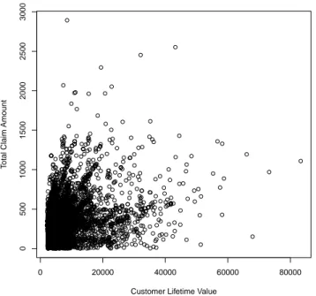
high quantile and a given value for the covariate income, X. In our analysis, we only use the data with a nonzero value for the income variable, leading to n “ 6817 observations. The scatterplot of total claim amount versus customer lifetime value, shown in Figure 7, indicates a positive association between these variables. In order to verify the Pareto-type behavior of Yp1q, we construct the local Pareto quantile plots of the Yp1q data for which X P r30000, 40000s
and X P r70000, 80000s, respectively, see Figure 8, top row. Clearly, the local Pareto quan-tile plots become approximately linear in the largest observations, which confirms underlying Pareto-type distributions (see Beirlant et al., 2004, for a general discussion of Pareto quantile-quantile plots). Also shown in Figure 8 are the Hill estimates of the total claim amount for which X P r30000, 40000s and X P r70000, 80000s, respectively (bottom row). When focusing on the stable horizontal parts of these plots we can clearly see that the theoretical requirement γ1px0q ă 0.5 is satisfied. Also for Yp2qthe local Pareto quantile plots become linear in the largest
observations, indicating underlying Pareto-type distributions, though the linearity is only in the very largest observations; see Figure 9. Similar local Pareto quantile plots were obtained at other incomes. Next, we investigate the asymptotic dependence assumption by plotting, in Fig-ure 10, pRp2, 2|x0q given in (8) as a function of k, at x0 “ 35000 and x0 “ 75000. Clearly, the
displays show a positive estimate for Rp2, 2|x0q, which gives evidence of asymptotic dependence
of Yp1q and Yp2q given X “ x
0. Finally, we illustrate the estimation of the conditional marginal
expected shortfall of total claim amount given a customer lifetime value that exceeds a high quantile and given a certain income. In Figure 11, we show pθppx0q as a function of income for
p “ 0.1% and p “ 0.05%. To obtain the estimate for θppx0q, we firstly obtain pγ1,k1px0q. This is
done by plottingγp1,k1px0q as a function of k1, followed by determining k1 by applying a stability
criterion as described in Goegebeur et al. (2019). Then, the k-value for the estimation of the conditional marginal expected shortfall at a given x0 was obtained in a similar way. Note that
0 20000 40000 60000 80000 0 500 1000 1500 2000 2500 3000
Customer Lifetime Value
T
otal Claim Amount
Figure 7: Vehicle insurance dataset. Scatterplot of total claim amount versus customer lifetime value.
criterion as in the simulation section, resulting in hn “ 26950. From Figure 11 we see that
smaller values of p lead to larger estimates of the conditional marginal expected shortfall, as expected. Overall, the conditional marginal expected shortfall is quite stable for incomes up to 60000 whereafter it shows a slight decrease. In Figure 11 we show also pointwise 95% confidence intervals for θppx0q based on (7). As expected, the confidence intervals are clearly wider for
p “ 0.05% than for p “ 0.1%, reflecting the higher uncertainty of the estimate at p “ 0.05% due to the fact that the estimation is based on fewer observations.
5
Preliminary results
To be self contained, we recall below Theorem 2.3 from Goegebeur et al. (2020) which states the weak convergence of θk
npx0q. Note that this theorem has been adjusted due to our Assumption
pSq which is slightly different from the one in the latter paper, and the additional H¨older-type condition on the R´function in Assumption pHq.
Theorem 5.1 Assume pDq, pHq, pKq, pSq with x Ñ Rpy1, y2|xq being a continuous function,
and y Ñ Fjpy|x0q, j “ 1, 2, are strictly increasing. Let x0 P IntpSXq such that fXpx0q ą 0.
0 1 2 3 4 5 6 7 1 2 3 4 5 6 7 8
Standard Exponential Quantiles
log(T
otal Claim Amount)
0 1 2 3 4 5 6 1 2 3 4 5 6 7
Standard Exponential Quantiles
log(T
otal Claim Amount)
0 200 400 600 800 0.0 0.2 0.4 0.6 0.8 1.0 k Hill Estimate 0 100 200 300 400 500 600 700 0.0 0.2 0.4 0.6 0.8 1.0 k Hill Estimate
Figure 8: Vehicle insurance dataset. Top row: Pareto quantile plots of the total claim amount for which income P r30000, 40000s (left) and income P r70000, 80000s (right). Bottom row: Hill estimates of the total claim amount for which income P r30000, 40000s (left) and income P r70000, 80000s (right).
0 1 2 3 4 5 6 7 8.0 8.5 9.0 9.5 10.0 10.5 11.0
Standard Exponential Quantiles
log(Customer Lif etime V alue) 0 1 2 3 4 5 6 8.0 8.5 9.0 9.5 10.0 10.5 11.0
Standard Exponential Quantiles
log(Customer Lif
etime V
alue)
Figure 9: Vehicle insurance dataset. Pareto quantile plots of the customer lifetime value for which income P r30000, 40000s (left) and income P r70000, 80000s (right).
0 100 200 300 400 0.0 0.2 0.4 0.6 0.8 1.0 k R 0 100 200 300 400 0.0 0.2 0.4 0.6 0.8 1.0 k R
Figure 10: Vehicle insurance dataset. pRp2, 2|x0q as a function of k, for x0 “ 35000 (left) and
Income T otal claim p=0.1% 10000 15000 20000 25000 30000 35000 40000 45000 50000 55000 60000 65000 70000 75000 80000 85000 90000 95000 100000 0 500 1000 1500 2000 2500 3000 3500 4000 Income T otal claim p=0.05% 10000 15000 20000 25000 30000 35000 40000 45000 50000 55000 60000 65000 70000 75000 80000 85000 90000 95000 100000 0 500 1000 1500 2000 2500 3000 3500 4000
Figure 11: Vehicle insurance dataset. pθppx0q along with pointwise 95% confidence intervals for
θppx0q at several values of x0 for p “ 0.1% (left), p “ 0.05% (right).
functions at infinity, with α P p0, 1q and max ˆ α d ` 2γ1px0qpηR^ ηA1^ ηγ1q , α d ` 2p1 ´ γ1px0qqpηA2^ ηγ2^ ηB2 ^ ηε2 ^ ηfXq , α d´ 2p1 ´ αqγ12px0qβ1px0q d ` dpβ1px0q ` εqγ1px0q ,α ´ 2p1 ´ αqpγ1px0q ^ pβ2px0qγ2px0qq ^ p´τ qq d ¯ ă ∆ ă α d. Then, for γ1px0q ă 1{2, we have
b khd n ˜ θk npx0q θk npx0q ´ 1 ¸ ´p1 ´ γ1px0qq W p8, 1q fXpx0q ` 1 fXpx0q ş8 0 W ps, 1qds ´γ1px0q ş8 0 Rps, 1|x0qds´γ1px0q . Now, remark that, assuming that F1py|x0q is strictly increasing in y, we have
p γ1,k1px0q “ 1 p fnpx0q 1 k1 n ÿ i“1 Khnpx0´ Xiq żYip1q p U1pn{k1|x0q 1 udu1ltYip1qě pU1pn{k1|x0qu “ 1 p fnpx0q ż8 p U1pn{k1|x0q 1 k1 n ÿ i“1 Khnpx0´ Xiq 1 u1ltYip1qěuudu “ 1 p fnpx0q ż8 p U1pn{k1|x0q 1 k1 n ÿ i“1 Khnpx0´ Xiq1ltF 1pYip1q|x0qďk1n k1n F1pu|x0qu 1 udu “ γ1px0q f px q ż1 1 k n ÿ Khnpx0´ Xiq1ltF 1pYip1q|x0qďk1 n F1pz´γ1px0qUp1pn{k1|x0q|x0qu 1 zdz
where Tnpy|x0q :“ 1 k1 n ÿ i“1 Khnpx0´ Xiq1ltF1pYp1q i |x0qďk1{n yu , and psnpz|x0q :“ n k1 F1 ´ z´γ1px0qUp 1pn{k1|x0q ˇ ˇ ˇx0 ¯ .
Thus we need to study the asymptotic properties of Tnpy|x0q,spnpz|x0q and pU1pn{k1|x0q.
We start by showing the weak convergence of the process based on Tnpy|x0q, first when the
process is centered around its expectation (Theorem 5.2) and then when it is centered around the dominant term of its expectation (Corollary 5.1).
Theorem 5.2 Assume pDq, pHq, pKq, and x0 P Int(SXq with fXpx0q ą 0, and y Ñ F1py|x0q
is strictly increasing. Consider sequences k1 Ñ 8 and hn Ñ 0 as n Ñ 8, in such a way that
k1{n Ñ 0, k1hdnÑ 8 and h ηγ1^ηε1
n ln n{k1 Ñ 0. Then for η P r0, 1{2q, we have,
b k1hdn
ˆ Tnpy|x0q ´ EpTnpy|x0qq
yη
˙
W py, 8q
yη , (10)
in Dpp0, T sq, for any T ą 0.
Proposition 5.1 Assume pDq, pHq, pKq, and x0 P Int(SXq with fXpx0q ą 0. Consider
se-quences k1Ñ 8 and hnÑ 0 as n Ñ 8, in such a way that k1{n Ñ 0, and h ηγ1^ηε1
n ln n{k1Ñ 0.
Then for η P r0, 1q, we have, E pTnpy|x0qq yη “ y 1´ηf Xpx0q ` O ´ hηnfX^ηA1 ¯ ` O ˆ hηnγ1ln n k1 ˙ ` O ˆˇ ˇ ˇ ˇ δ1 ˆ U1 ˆ n k1 ˇ ˇ ˇx0 ˙ˇ ˇ ˇx0 ˙ˇ ˇ ˇ ˇ hηnB1 ˙ `O ˆˇ ˇ ˇ ˇδ1 ˆ U1 ˆ n k1 ˇ ˇ ˇx0 ˙ ˇ ˇ ˇx0 ˙ˇ ˇ ˇ ˇh ηε1 n ln n k1 ˙ , where the O–terms are uniform in y P p0, T s, for any T ą 0.
Corollary 5.1 Assume pDq, pHq, pKq, x0 P IntpSXq with fXpx0q ą 0, and y Ñ F1py|x0q
is strictly increasing. Consider sequences k1 Ñ 8 and hn Ñ 0 as n Ñ 8, in such a way
that k1{n Ñ 0, k1hdn Ñ 8, h ηε1 n ln n{k1 Ñ 0, a k1hdnh ηfX^ηA1 n Ñ 0, a k1hdnh ηγ1 n ln n{k1 Ñ 0, a k1hdn|δ1pU1pn{k1|x0q|x0q|h ηB1 n Ñ 0, and a k1hdn|δ1pU1pn{k1|x0q|x0q|h ηε1 n ln n{k1 Ñ 0. Then for η P r0, 1{2q, we have, b k1hdn ˆ Tnpy|x0q yη ´ y 1´ηf Xpx0q ˙ W py, 8q yη , in Dpp0, T sq, for any T ą 0.
In the sequel, for convenient representation, the limiting process in Theorem 5.2 and Corollary 5.1 will be defined on the same probability space as the original random variables, via the Skorohod construction, but it should be kept in mind that it is only in distribution equal to
the original process. The Skorohod representation theorem gives then, with keeping the same notation, that sup yPp0,T s ˇ ˇ ˇ ˇ b k1hdn ˆ Tnpy|x0q yη ´ y 1´ηf Xpx0q ˙ ´W py, 8q yη ˇ ˇ ˇ ˇÑ 0 a.s. , as n Ñ 8.
For the intermediate quantile estimate pU1pn{k|x0q, we recall Lemma 5.6 from Goegebeur et al.
(2020), which is used several times in our proofs, and which states the weak convergence of p
un:“ pU1pn{k1|x0q{U1pn{k1|x0q.
Lemma 5.1 Assume pDq, pHq, pKq, x0 P IntpSXq with fXpx0q ą 0 and y Ñ F1py|x0q is
strictly increasing. Consider sequences k1 Ñ 8 and hn Ñ 0 as n Ñ 8, in such a way that
k1{n Ñ 0, k1hdn Ñ 8, h ηε1 n ln n{k1 Ñ 0, a k1hdnh ηfX^ηA1 n Ñ 0, a k1hdnh ηγ1 n ln n{k1 Ñ 0, a k1hdn|δ1pU1pn{k1|x0q|x0q| Ñ 0. Then, as n Ñ 8, we have b k1hdnppun´ 1q γ1px0qW p1, 8q fXpx0q .
From Lemma 5.1, we can show now the uniform convergence in probability ofpsnpz|x0q towards z for any z P p0, T s.
Lemma 5.2 Under the assumptions of Lemma 5.1, for any T ą 0, we have sup
zPp0,T s
|psnpz|x0q ´ z| “ oPp1q.
Proof of the preliminary results
Proof of Theorem 5.2. Recall that Tnpy|x0q yη “ 1 k1 n ÿ i“1 Khnpx0´ Xiq1ltF 1pYip1q|x0qďk1nyu 1 yη.
The proof of Theorem 5.2 follows the lines of proof of Theorem 2.1 in Goegebeur et al. (2020). Below, we only outline the main differences and refer to the latter paper otherwise. To start, we need some notations from empirical process theory with changing function classes, see for instance van der Vaart and Wellner (1996). Let P be the distribution measure of pYp1q, Xq,
and denote the expected value under P as P f :“ş fdP for any real-valued measurable function f : R ˆ Rd Ñ R. For a function class F , let Nrspε, F , L2pP qq, denote the minimal number of
ε´brackets needed to cover F . The bracketing integral is then defined as Jrspδ, F , L2pP qq “
żδ
0
b
where fn,ypu, zq :“ d nhd n k1 Khnpx0´ zq1ltF 1pu|x0qďk1nyu 1 yη.
Denote also by Fn an envelope function of the class Fn. Now, according to Theorem 19.28
in van der Vaart (1998), the weak convergence of the stochastic process (10) follows from the following four conditions. Let ρx0 be a semimetric, possibly depending on x0, making p0, T s
totally bounded. We have to prove that sup
ρx0py,¯yqďδn
P pfn,y´ fn,¯yq2 ÝÑ 0 for every δnŒ 0, (11)
P Fn2 “ Op1q, (12)
P Fn21ltFnąε?
nu ÝÑ 0 for every ε ą 0, (13)
and
Jrspδn, Fn, L2pP qq ÝÑ 0 for every δnŒ 0. (14)
We start with verifying condition p11q, with ρx0py, yq :“ |y ´ y|. Without loss of generality, we
may assume that y ď y. We have
P pfn,y´ fn,yq2 “ nhdn k1 E » –Kh2 npx0´ Xq ˜ 1l tF1pYp1q|x0qďk1nyu yη ´ 1l tF1pYp1q|x0qďk1nyu yη ¸2fi fl.
We consider now two cases. Case 1: y ď δn. We have ˜ 1l tF1pYp1q|x0qďk1nyu yη ´ 1l tF1pYp1q|x0qďk1nyu yη ¸2 ď 3 1l tF1pYp1q|x0qďk1nyu y2η ` 1l tF1pYp1q|x0qďk1nyu y2η .
This implies that P pfn,y´ fn,yq2 ď 3 nhdn k1 E ˜ Kh2npx0´ Xq 1l tF1pYp1q|x0qďk1nyu y2η ¸ `nh d n k1 E ˜ Kh2npx0´ Xq 1l tF1pYp1q|x0qďk1nyu y2η ¸ “ 3nh d n k1 ż Rd 1 h2d n K2ˆ x0´ v hn ˙P ´ F1pYp1q|x0q ď kn1y|X “ v ¯ y2η fXpvqdv `nh d n k1 ż Rd 1 h2d n K2ˆ x0´ v hn ˙P ´ F1pYp1q|x0q ď kn1y|X “ v ¯ y2η fXpvqdv “ 3 n k1 ż SK K2pvq P ´ F1pYp1q|x0q ď kn1y|X “ x0´ hnv ¯ y2η fXpx0´ hnvqdv `n k1 ż SK K2pvq P ´ F1pYp1q|x0q ď kn1y|X “ x0´ hnv ¯ y2η fXpx0´ hnvqdv. Since P ´ F1pYp1q|x0q ď kn1y ˇ ˇ ˇX “ x0´ hnv ¯ “ F1 ´ U1pkn1y|x0q ˇ ˇ ˇx0´ hnv ¯ , this yields P pfn,y´ fn,yq2 ď 3 y1´2η ż SK K2pvqfXpx0´ hnvqdv `3 ż SK K2pvq „ 1 y2η n k1 F1 ˆ U1 ˆ n k1y ˇ ˇ ˇx0 ˙ ˇ ˇ ˇx0´ hnv ˙ ´ y1´2η fXpx0´ hnvqdv `y1´2η ż SK K2pvqfXpx0´ hnvqdv ` ż SK K2pvq „ 1 y2η n k1 F1 ˆ U1 ˆ n k1y ˇ ˇ ˇx0 ˙ˇ ˇ ˇx0´ hnv ˙ ´ y1´2η fXpx0´ hnvqdv.
Using Lemma 5.1 in Goegebeur et al. (2020) and the fact that ρx0py, yq ď δn which implies
y ď 2δn, we get
P pfn,y´ fn,yq2ď 5 δ1´2ηn
ż
SK
K2pvqfXpx0´ hnvqdv ` op1q,
where the op1q´term does not depend on y and y. Case 2: y ą δn. In that case
˜ 1l tF1pYp1q|x0qďk1nyu yη ´ 1l tF1pYp1q|x0qďk1nyu yη ¸2 ď ˆ 1 yη ´ 1 yη ˙2 1l tF1pYp1q|x0qďk1yu
from which we deduce that P pfn,y´ fn,yq2 ď pyη ´ yηq2 pyyq2η ż SK K2pvqn k1 F1pU1pn{pk1yq|x0q|x0´ hnvq fXpx0´ hnvqdv ` 1 y2η n k1 ż SK K2pvqPˆ k1 ny ď F1pY p1q |x0q ď k1 ny ˇ ˇ ˇ ˇX “ x0´ hnv ˙ fXpx0´ hnvqdv.
These two terms on the right-hand side of the above inequality can be handled similarly as those in case 3 in the proof of Theorem 2.1 in Goegebeur et al. (2020).
Now, a natural envelope function of the class Fn is
Fnpu, zq :“ d nhd n k1 Khnpx0´ zq 1ltF 1pu|x0qďk1T {nu rpn{k1q F1pu|x0qsη .
Thus, according again to the proof of Theorem 2.1 in Goegebeur et al. (2020), conditions p12q and p13q are satisfied.
Finally, we need to show condition p14q. Without loss of generality we assume T “ 1. Consider for a, θ ă 1:
Fp1q
n paq :“ tfn,yP Fn: y ď au,
and
Fp2q
n p`q :“ tfn,yP Fn: θ``1 ď y ď θ`u,
where ` “ 0, . . . , tln a{ ln θu .
The class Fnp1qpaq has been already studied in the proof of Theorem 2.1 in Goegebeur et al.
(2020) and Fnp2qp`q can be dealt with similar arguments as for Fnp`, mq from the latter paper,
since we have the following bounds
unpu, zq :“ d nhd n k1 Khnpx0´ zq 1ltF 1pu|x0qďk1{n θ``1u θ`η ď fn,ypu, zq ď d nhd n k1 Khnpx0´ zq 1ltF 1pu|x0qďk1{n θ`u θp``1qη “: unpu, zq.
Proof of Proposition 5.1. We have E rTnpy|x0qs yη “ 1 yη n k1E ” Khnpx0´ Xq1ltF 1pYp1q|x0qďk1nyu ı “ 1 yη n k1 ż Rd 1 hd n Kˆ x0´ u hn ˙ P ˆ F1 ´ Yp1q ˇ ˇ ˇx0 ¯ ď k1 ny ˇ ˇ ˇX “ u ˙ fXpuqdu “ 1 yη n k1 ż SK KpuqF1 ˆ U1 ˆ n k1y ˇ ˇ ˇx0 ˙ˇ ˇ ˇx0´ hnu ˙ fXpx0´ hnuqdu “ y1´ηfXpx0q ` y1´η ż SK Kpuq rfXpx0´ hnuq ´ fXpx0qs du `fXpx0q ż SK Kpuq » – n k1F1 ´ U1 ´ n k1y ˇ ˇ ˇx0 ¯ˇ ˇ ˇx0´ hnu ¯ yη ´ y 1´η fi fldu ` ż SK Kpuq » – n k1F1 ´ U1 ´ n k1y ˇ ˇ ˇx0 ¯ˇ ˇ ˇx0´ hnu ¯ yη ´ y 1´η fi flrfXpx0´ hnuq ´ fXpx0qs du.
Following the lines of proof of Lemma 5.1 in Goegebeur et al. (2020), we have ˇ ˇ ˇ ˇ ˇ ˇ n k1F1 ´ U1 ´ n k1y ˇ ˇ ˇx0 ¯ˇ ˇ ˇx0´ hnu ¯ yη ´ y 1´η ˇ ˇ ˇ ˇ ˇ ˇ “ O ´ hηnA1 ¯ ` O ˆ hηnγ1ln n k1 ˙ ` O ˆˇ ˇ ˇ ˇδ1 ˆ U1 ˆ n k1 ˇ ˇ ˇx0 ˙ ˇ ˇ ˇx0 ˙ˇ ˇ ˇ ˇh ηB1 n ˙ `O ˆˇ ˇ ˇ ˇδ1 ˆ U1 ˆ n k1 ˇ ˇ ˇx0 ˙ ˇ ˇ ˇx0 ˙ˇ ˇ ˇ ˇh ηε1 n ln n k1 ˙ , with O´terms which are uniform in y P p0, T s, for any T ą 0. This yields Proposition 5.1.
Proof of Corollary 5.1. Using the decomposition b k1hdn ˆ Tnpy|x0q yη ´ y 1´ηf Xpx0q ˙ “ b k1hdn
ˆ Tnpy|x0q ´ EpTnpy|x0qq
yη ˙ ` b k1hdn ˆ E pTnpy|x0qq yη ´ y 1´ηf Xpx0q ˙ , combined with Theorem 5.2 and Proposition 5.1 yields Corollary 5.1.
Proof of Lemma 5.2. We have, for z P p0, T s and any ε ą 0 and ζ P p0, β1px0qs |psnpz|x0q ´ z| “ ˇ ˇ ˇ ˇ n k1 F1 ´ z´γ1px0q p unU1pn{k1|x0q ˇ ˇ ˇx0 ¯ ´ z ˇ ˇ ˇ ˇ “ ˇ ˇ ˇ ˇ ˇ ˇ F1 ´ z´γ1px0q p unU1pn{k1|x0q ˇ ˇ ˇx0 ¯ F1 ´ U1pn{k1|x0q ˇ ˇ ˇx0 ¯ ´ z ˇ ˇ ˇ ˇ ˇ ˇ ď z ˇ ˇ ˇpu ´1{γ1px0q n ´ 1 ˇ ˇ ˇ 1 `γ 1 1px0qδ1 ´ z´γ1px0q p unU1pn{k1|x0q ˇ ˇ ˇx0 ¯ 1 `γ 1 1px0qδ1 ´ U1pn{k1|x0q ˇ ˇ ˇx0 ¯ ` z γ1px0q ˇ ˇ ˇδ1 ´ U1pn{k1|x0q ˇ ˇ ˇx0 ¯ˇ ˇ ˇ 1 `γ 1 1px0qδ1 ´ U1pn{k1|x0q ˇ ˇ ˇx0 ¯ ˇ ˇ ˇ ˇ ˇ ˇ δ1 ´ z´γ1px0q p unU1pn{k1|x0q ˇ ˇ ˇx0 ¯ δ1 ´ U1pn{k1|x0q ˇ ˇ ˇx0 ¯ ´ 1 ˇ ˇ ˇ ˇ ˇ ˇ ď C T ˇ ˇ ˇpu ´1{γ1px0q n ´ 1 ˇ ˇ ˇ `C T ˇ ˇ ˇδ1 ´ U1pn{k1|x0q ˇ ˇ ˇx0 ¯ˇ ˇ ˇ $ & % ˇ ˇ ˇ ˇ ˇ ˇ δ1 ´ z´γ1px0q p unU1pn{k1|x0q ˇ ˇ ˇx0 ¯ δ1 ´ U1pn{k1|x0q ˇ ˇ ˇx0 ¯ ´ ´ z´γ1px0q p un ¯´β1px0q ˇ ˇ ˇ ˇ ˇ ˇ ` ˇ ˇ ˇ ˇ ´ z´γ1px0q p un ¯´β1px0q ´ 1 ˇ ˇ ˇ ˇ * ď C T ˇ ˇ ˇpu ´1{γ1px0q n ´ 1 ˇ ˇ ˇ `C ε ˇ ˇ ˇδ1 ´ U1pn{k1|x0q ˇ ˇ ˇx0 ¯ˇ ˇ ˇ T 1`γ1px0qβ1px0q˘γ1px0qζ p u´β1px0q˘ζ n `C ˇ ˇ ˇδ1 ´ U1pn{k1|x0q ˇ ˇ ˇx0 ¯ˇ ˇ ˇ T ! Tγ1px0qβ1px0q p u´β1px0q n ` 1 ) ,
for n large, with arbitrary large probability, by Proposition B.1.10 in de Haan and Ferreira (2006). In the above, the notation a˘‚ means a‚ if a ě 1 and a´‚ if a ă 1. Using Lemma 5.1,
6
Proofs of the main results
Proof of Theorem 2.1. Using (9), we have the following decomposition b k1hdnppγ1,k1px0q ´ γ1px0qq “ γ1px0q fXpx0q ż1 0 W pz, 8q1 zdz `γ1px0q b k1hdn ż1 0 „ p snpz|x0q z ´ 1 dz `γ1px0q fXpx0q ż1 0 rW ppsnpz|x0q, 8q ´ W pz, 8qs 1 zdz `γ1px0q ż1 0 "b k1hdn „ Tnppsnpz|x0q|x0q fXpx0qpsηnpz|x0q ´ps 1´η n pz|x0q ´W ppsnpz|x0q, 8q fXpx0qpsηnpz|x0q * p sηnpz|x0q z dz ´ γ1px0q fXpx0q pfnpx0q ż1 0 Tnppsnpz|x0q|x0q 1 zdz c k1 n b nhd n ´ p fnpx0q ´ fXpx0q ¯ “: γ1px0q fXpx0q ż1 0 W pz, 8q1 zdz ` 4 ÿ i“1 Ti,n.
We study each term separately.
Concerning T1,n, following the lines of proof of Lemma 5.2, we have
T1,n“ γ1px0q b k1hdn ” p u´1{γ1px0q n ´ 1 ı ` oPp1q. Now, combining Lemma 5.1 with a Taylor expansion, we have
T1,n ´
γ1px0q
fXpx0q
W p1, 8q. Concerning T2,n, for δ P p0, 1q, we use the decomposition
T2,n “ γ1px0q fXpx0q "żδ 0 rW ppsnpz|x0q, 8q ´ W pz, 8qs 1 zdz ` ż1 δ rW ppsnpz|x0q, 8q ´ W pz, 8qs 1 zdz * “: T2,np1q` T2,np2q.
Using Lemma 5.2 combined with Potter’s bounds (see Proposition B.1.9 (5) in de Haan and Ferreira, 2006), we have for any ζ P p0, 1{γ1px0qq, for n large, and with arbitrary large probability
|T2,np1q| ď γ1px0q fXpx0q sup zPp0,2s |W pz, 8q| zη „żδ 0 p sηnpz|x0q z dz ` δη η ď C żδ1 z ” z´γ1px0q p un ıηp˘ζ´1{γ1px0qq dz ` Cδη
Now, concerning T2,np2q, remark that following the lines of proof of Lemma 5.2, we have sup zPrδ,1s ´ k1hdn ¯1{4 |psnpz|x0q ´ z| “ oPp1q,
from which we deduce that, for any ξ ą 0 P ˜ sup zPrδ,1s |W ppsnpz|x0q, 8q ´ W pz, 8q| ą ξ ¸ ď P ˜ sup zPrδ,1s |W ppsnpz|x0q, 8q ´ W pz, 8q| ą ξ, sup zPrδ,1s |psnpz|x0q ´ z| ď 1 pk1hdnq1{4 ¸ `P ˜ sup zPrδ,1s |psnpz|x0q ´ z| ą 1 pk1hdnq1{4 ¸ ď P ¨ ˝ sup zPrδ,1s,|y´z|ď 1 pk1hdnq1{4 |W py, 8q ´ W pz, 8q| ą ξ ˛ ‚` P ˜ sup zPrδ,1s |psnpz|x0q ´ z| ą 1 pk1hdnq1{4 ¸ “ op1q,
by the continuity of W p¨, 8q. This implies that |T2,np2q| ď ε ln1
δ “ ´ ε ηln ε. Hence, T2,n“ oPp1q.
Concerning T3,n, from Lemma 5.2, we have, for n large, with arbitrary large probability
|T3,n| ď γ1px0q fXpx0q sup yPp0,2s ˇ ˇ ˇ ˇ b k1hdn ˆ Tnpy|x0q yη ´ y 1´ηf Xpx0q ˙ ´W py, 8q yη ˇ ˇ ˇ ˇ ż1 0 p sηnpz|x0q z dz.
Then, by Corollary 5.1 combined with the Skorohod representation theorem, we can conclude that T3,n“ oPp1q.
Finally, T4,n“ oPp1q using the properties of the kernel density estimator.
This achieves the proof of Theorem 2.1.
Proof of Theorem 2.2. We use the decomposition
p θppx0q θppx0q “ # ˆ k np ˙pγ1,k1px0q´γ1px0q+ loooooooooooooomoooooooooooooon T5,n # θk npx0q θk npx0q + looooomooooon T6,n $ & % pnpkqγ1px0qθ k npx0q θppx0q , . -loooooooooooomoooooooooooon T7,n ,
from which we deduce that p θppx0q θppx0q ´ 1 “ # ˆ k np ˙pγ1,k1px0q´γ1px0q ´ 1 + T6,nT7,n` # θk npx0q θk npx0q ´ 1 + T7,n` $ & % pnpkqγ1px0qθ k npx0q θppx0q ´ 1 , . -.(15)
We will study the three terms pTi,n´ 1q, i “ 5, 6, 7, separately.
Concerning the term pT5,n´ 1q, remark that, assuming ln k{pnpq? k1hdn
ÝÑ 0 and using Theorem 2.1, we have ˆ k np ˙pγ1,k1px0q´γ1px0q ´ 1 “ exp # b k1hdnrpγ1,k1px0q ´ γ1px0qs ln k{pnpq a k1hdn + ´ 1 “ b k1hdnrpγ1,k1px0q ´ γ1px0qs ln k{pnpq a k1hdn p1 ` oPp1qq ,
from which we deduce that a k1hdn ln k{pnpq # ˆ k np ˙pγ1,k1px0q´γ1px0q ´ 1 + γ1px0q fXpx0q „ż1 0 W pz, 8q1 zdz ´ W p1, 8q . (16)
The asymptotic behavior of the term pT6,n´ 1q has been already established in Theorem 5.1.
Now, concerning the term pT7,n´ 1q, remark that
pnpk qγ1px0qθ k{npx0q θppx0q ´ 1 “ ˆ θk{npx0q{U1pn{k|x0q θppx0q{U1p1{p|x0q ´ 1 ˙U 1pn{k|x0qpnpkqγ1px0q U1p1{p|x0q ` U1pn{k|x0qpnpkqγ1px0q U1p1{p|x0q ´ 1. (17) Under assumption pDq, (2) yields
U1pn{k|x0qpnpkqγ1px0q U1p1{p|x0q ´ 1 “ 1 ` a1pn{k|x0q 1 ` a1p1{p|x0q ´ 1 “ o ˜ 1 a khd n ¸ , (18) sinceakhd n|δ1pU1pn{k|x0q|x0q| Ñ 0 and a khd
Moreover θk{npx0q U1pn{k|x0q “ ż8 0 n kP ´ Yp1q ą y1, Yp2qě U2pn{k|x0q ˇ ˇ ˇx0 ¯ dy 1 U1pn{k|x0q “ ż8 0 n kP ˆ 1 ´ F1pYp1q|x0q ă 1 ´ F1py1|x0q, 1 ´ F2pYp2q|x0q ď k n ˇ ˇ ˇx0 ˙ dy1 U1pn{k|x0q “ ż8 0 Rn{k ´n kr1 ´ F1py1|x0qs , 1 ˇ ˇ ˇx0 ¯ dy 1 U1pn{k|x0q “ ´ ż8 0 Rn{k ´n k ” 1 ´ F1pz1´γ1px0qU1pn{k|x0q|x0q ı , 1 ˇ ˇ ˇx0 ¯ dz´γ1px0q 1 “ ´ ż8 0 Rpz1, 1|x0qdz1´γ1px0q ´ ż8 0 ” Rn{k ´n k ” 1 ´ F1pz1´γ1px0qU1pn{k|x0q|x0q ı , 1 ˇ ˇ ˇx0 ¯ ´R ´n k ” 1 ´ F1pz1´γ1px0qU1pn{k|x0q|x0q ı , 1 ˇ ˇ ˇx0 ¯ı dz´γ1px0q 1 ´ ż8 0 ” R ´n k ” 1 ´ F1pz´γ1 1px0qU1pn{k|x0q|x0q ı , 1 ˇ ˇ ˇx0 ¯ ´ R pz1, 1|x0q ı dz´γ1px0q 1 “: ´ ż8 0 Rpz1, 1|x0qdz1´γ1px0q` T8,n` T9,n. Now, by Assumption pSq |T8,n| ď sup xPBpx0,hnq sup 0ăy1ă8,12ďy2ď2 |Rn{kpy1, y2|xq ´ Rpy1, y2|xq| y1β^ 1 ˆ ˇ ˇ ˇ ˇ ż8 0 ˆ !n k ” 1 ´ F1pz1´γ1px0qU1pn{k|x0q|x0q ı)β ^ 1 ˙ dz´γ1px0q 1 ˇ ˇ ˇ ˇ “ O ´´n k ¯τ¯ “ o ˜ 1 a khd n ¸ ,
by our assumptions on the sequence k, and |T9,n| ď sup 1 2ďy2ď2 ˇ ˇ ˇ ˇ ż8 0 ” R ´n k ” 1 ´ F1pz1´γ1px0qU1pn{k|x0q|x0q ı , y2 ˇ ˇ ˇx0 ¯ ´ R pz1, y2|x0q ı dz´γ1px0q 1 ˇ ˇ ˇ ˇ “ o ˜ 1 a khd n ¸ ,
by Lemma 5.4 in Goegebeur et al. (2020). Thus θk{npx0q U1pn{k|x0q “ ´ ż8 0 Rpz1, 1|x0qdz1´γ1px0q` o ˜ 1 a khd n ¸ . (19)
A similar type of property can be obtained for θppx0q instead of θk{npx0q. Indeed θppx0q U1p1{p|x0q “ ´ ż8 0 R1{pˆ 1 p ” 1 ´ F1pz1´γ1px0qU1p1{p|x0q|x0q ı , 1 ˇ ˇ ˇx0 ˙ dz´γ1px0q 1 “ ´ ż8 0 Rpz1, 1|x0qdz1´γ1px0q ´ ż8 0 „ R1{p ˆ 1 p ” 1 ´ F1pz1´γ1px0qU1p1{p|x0q|x0q ı , 1 ˇ ˇ ˇx0 ˙ ´Rˆ 1 p ” 1 ´ F1pz´γ1 1px0qU1p1{p|x0q|x0q ı , 1 ˇ ˇ ˇx0 ˙ dz´γ1px0q 1 ´ ż8 0 „ Rˆ 1 p ” 1 ´ F1pz1´γ1px0qU1p1{p|x0q|x0q ı , 1 ˇ ˇ ˇx0 ˙ ´ R pz1, 1|x0q dz´γ1px0q 1 “: ´ ż8 0 Rpz1, 1|x0qdz1´γ1px0q` T10,n` T11,n. Clearly T10,n “ Opp´τq “ o ˆ 1 ? khd n ˙
, by our assumptions on k and p. For T11,n, we follow the
lines of proof of the second part of Lemma 5.4 in Goegebeur et al. (2020), using the Lipschitz property of the function R, for TnÑ 8, we have
b khd n|T11,n| ď b khd n ˇ ˇ ˇ ˇ żTn 0 „ Rˆ 1 p ” 1 ´ F1 ´ z´γ1px0q 1 U1p1{p|x0q ˇ ˇ ˇx0 ¯ı , 1 ˇ ˇ ˇx0 ˙ ´ Rpz1, 1|x0q dz´γ1px0q 1 ˇ ˇ ˇ ˇ ` b khd n ˇ ˇ ˇ ˇ ż8 Tn „ Rˆ 1 p ” 1 ´ F1 ´ z´γ1px0q 1 U1p1{p|x0q ˇ ˇ ˇx0 ¯ı , 1 ˇ ˇ ˇx0 ˙ ´ Rpz1, 1|x0q dz´γ1px0q 1 ˇ ˇ ˇ ˇ ď ´ b khd n żTn 0 ˇ ˇ ˇ ˇ 1 p ” 1 ´ F1 ´ z´γ1px0q 1 U1p1{p|x0q ˇ ˇ ˇx0 ¯ı ´ z1 ˇ ˇ ˇ ˇ dz´γ1px0q 1 `2 sup z1ě0 Rpz1, 1|x0q b khd nTn´γ1px0q ď ´ b khd n ˇ ˇ ˇδ1 ´ U1 ´ 1 p ˇ ˇ ˇx0 ¯ˇ ˇ ˇx0 ¯ˇ ˇ ˇ ˇ ˇ ˇγ1px0q ` δ1 ´ U1 ´ 1 p ˇ ˇ ˇx0 ¯ˇ ˇ ˇx0 ¯ˇ ˇ ˇ żTn 0 z1 ˇ ˇ ˇ ˇ ˇ ˇ δ1 ´ z´γ1px0q 1 U1 ´ 1 p ˇ ˇ ˇx0 ¯ˇ ˇ ˇx0 ¯ δ1 ´ U1 ´ 1 p ˇ ˇ ˇx0 ¯ |x0 ¯ ´ 1 ˇ ˇ ˇ ˇ ˇ ˇ dz´γ1px0q 1 `C b khd nTn´γ1px0q ď C b khd n ˇ ˇ ˇ ˇ δ1 ˆ U1 ˆ 1 p ˇ ˇ ˇx0 ˙ˇ ˇ ˇx0 ˙ˇ ˇ ˇ ˇ T1´γ1px0q`pβ1px0q`εqγ1px0q n ` C b khd nTn´γ1px0q ď C b khd n ˇ ˇ ˇδ1 ´ U1 ´n k ˇ ˇ ˇx0 ¯ˇ ˇ ˇx0 ¯ˇ ˇ ˇ T 1´γ1px0q`pβ1px0q`εqγ1px0q n ` C b khd nTn´γ1px0q,
for n large. Then, if α and ∆ are chosen as stated in Theorem 2.2 and Tn“ nκ with κ chosen
such that
we have θppx0q U1p1{p|x0q “ ´ ż8 0 Rpz1, 1|x0qdz1´γ1px0q` o ˜ 1 a khd n ¸ . (20)
Combining (17), (18), (19) and (20), we deduce that pnpk qγ1px0qθ k{npx0q θppx0q ´ 1 “ o ˜ 1 a khd n ¸ . (21)
Finally, decomposition (15) combined with Theorem 5.1, (16) and (21) achieves the proof of Theorem 2.2.
Acknowledgement
The authors would like to thank the referees, the Associate Editor and editor for their helpful comments. The research of Armelle Guillou was supported by the French National Research Agency under the grant ANR-19-CE40-0013-01/ExtremReg project and an International Emerg-ing Action (IEA-00179).
References
Acharya, V., Pedersen, L., Philippon, T., Richardson, M. (2010). Measuring systemic risk. FRB of Cleveland Working Paper No. 10-02. https://ssrn.com/abstract=1595075.
Artzner, P., Delbaen, F., Eber, J-M., Heath, D. (1999). Coherent measures of risk, Mathemati-cal Finance, 9, 203–228.
Barg`es, M., Cossette, H., Marceau, ´E. (2009). TVar-based capital allocation with copulas, In-surance: Mathematics and Economics, 45, 310–324.
Beirlant, J., Goegebeur, Y., Segers, J., Teugels, J. (2004). Statistics of Extremes: Theory and Applications, Wiley.
Beirlant, J., Joossens, E., Segers, J. (2009). Second-order refined peaks-over-threshold modelling for heavy-tailed distributions, Journal of Statistical Planning and Inference, 139, 2800–2815. Brazaukas, V., Jones, B., Puri, L., Zitikis, R. (2008). Estimating conditional tail expectation with actuarial applications in view, Journal of Statistical Planning and Inference, 128, 3590– 3604.
Cai, J.J., Einmahl, J.H.J., de Haan, L., Zhou, C. (2015). Estimation of the marginal expected shortfall: the mean when a related variable is extreme, Journal of the Royal Statistical Society:
Series B (Statistical Methodology), 77, 417–442.
Cai, J., Li, H. (2005). Conditional tail expectations for multivariate phase-type distributions, Journal of Applied Probability, 42, 810–825.
Cai, J., Tan, K. S. (2007). Optimal retention for a stop-loss reinsurance under the VaR and CTE risk measures, Astin Bulletin, 37, 93–112.
Cousin, A., Di Bernardino, E. (2013). On multivariate extensions of value-at-risk, Journal of Multivariate Analysis, 119, 32–46.
Daouia, A., Gardes, L., Girard, S. (2013). On kernel smoothing for extremal quantile regression, Bernoulli, 19, 2557–2589.
Daouia, A., Gardes, L., Girard, S., Lekina, A. (2011). Kernel estimators of extreme level curves, TEST, 20, 311–333.
Das, B., Fasen-Hartmann, V. (2018). Risk contagion under regular variation and asymptotic tail independence, Journal of Multivariate Analysis, 165, 194–215.
Das, B., Fasen-Hartmann, V. (2019). Conditional excess risk measures and multivariate regular variation, Statistics & Risk Modeling 36, 1–23.
Di Bernardino, E., Prieur, C. (2018). Estimation of the multivariate conditional tail expecta-tion for extreme risk levels: Illustraexpecta-tion on environmental data sets, Environmetrics, 29, 7, 1–22. Drees, H. (2003). Extreme quantile estimation for dependent data, with applications to finance, Bernoulli, 9, 617–657.
El Methni, J., Gardes, L., Girard, S. (2014). Non-parametric estimation of extreme risk measures from conditional heavy-tailed distributions, Scandinavian Journal of Statistics, 41, 988–1012. El Methni, J., Gardes, L., Girard, S. (2018). Kernel estimation of extreme regression risk mea-sures, Electronic Journal of Statistics, 12, 359–398.
Escobar-Bach, M., Goegebeur, Y., Guillou, A. (2018a). Local robust estimation of the Pickands dependence function, Annals of Statistics, 46, 2806–2843.
Escobar-Bach, M., Goegebeur, Y., Guillou, A. (2018b). Local estimation of the conditional stable tail dependence function, Scandinavian Journal of Statistics, 45, 590–617.
Goegebeur, Y., Guillou, A., Qin, J. (2019). Bias-corrected estimation for conditional Pareto-type distributions with random right censoring, Extremes, 22, 459–498.
de Haan, L., Ferreira, A. (2006). Extreme value theory, an introduction, Springer.
Jorion, P. (2007). Value at risk: the new benchmark for managing financial risk, McGraw-Hill New York.
Hill, B.M. (1975). A simple general approach to inference about the tail of a distribution, Annals of Statistics, 5, 1163–1174.
Landsman, Z., Valdez, E. (2003). Tail conditional expectations for elliptical distributions, North American Actuarial Journal, 7, 55–71.
van der Vaart, A. W. (1998). Asymptotic statistics, Cambridge Series in Statistical and Proba-bilistic Mathematics, 3, Cambridge University Press, Cambridge.
van der Vaart, A. W., Wellner, J. A. (1996). Weak convergence and empirical processes, with applications to statistics, Springer Series in Statistics, Springer-Verlag, New York.
Yao, Q. (1999). Conditional predictive regions for stochastic processes, Technical report, Univer-sity of Kent at Canterbury, http://citeseerx.ist.psu.edu/viewdoc/download?doi=10.1.1. 45.2449&rep=rep1&type=pdf.