Measuring methods for groundwater, surface water and their interactions: a review

(1)

HAL Id: hal-00298739

https://hal.archives-ouvertes.fr/hal-00298739

Submitted on 21 Jul 2006

HAL is a multi-disciplinary open access

archive for the deposit and dissemination of sci-entific research documents, whether they are pub-lished or not. The documents may come from teaching and research institutions in France or abroad, or from public or private research centers.

L’archive ouverte pluridisciplinaire HAL, est destinée au dépôt et à la diffusion de documents scientifiques de niveau recherche, publiés ou non, émanant des établissements d’enseignement et de recherche français ou étrangers, des laboratoires publics ou privés.

Measuring methods for groundwater, surface water and

their interactions: a review

E. Kalbus, F. Reinstorf, M. Schirmer

To cite this version:

E. Kalbus, F. Reinstorf, M. Schirmer. Measuring methods for groundwater, surface water and their interactions: a review. Hydrology and Earth System Sciences Discussions, European Geosciences Union, 2006, 3 (4), pp.1809-1850. �hal-00298739�

(2)

HESSD

3, 1809–1850, 2006 Measuring groundwater-surface water interactions: a review E. Kalbus et al. Title Page Abstract Introduction Conclusions References Tables Figures J I J I Back Close

Full Screen / Esc

Printer-friendly Version

Interactive Discussion

Hydrol. Earth Syst. Sci. Discuss., 3, 1809–1850, 2006 www.hydrol-earth-syst-sci-discuss.net/3/1809/2006/ © Author(s) 2006. This work is licensed

under a Creative Commons License.

Hydrology and Earth System Sciences Discussions

Papers published in Hydrology and Earth System Sciences Discussions are under open-access review for the journal Hydrology and Earth System Sciences

Measuring methods for groundwater,

surface water and their interactions: a

review

E. Kalbus, F. Reinstorf, and M. Schirmer

Department of Hydrogeology, UFZ – Centre for Environmental Research Leipzig-Halle in the Helmholtz Association, Permoserstr. 15, 04318 Leipzig, Germany

Received: 9 May 2006 – Accepted: 2 June 2006 – Published: 21 July 2006 Correspondence to: E. Kalbus ([email protected])

(3)

HESSD

Full Screen / Esc

Abstract

Interactions between groundwater and surface water play a critical role in the function-ing of riparian ecosystems. In the context of sustainable river basin management it is crucial to understand and quantify exchange processes between groundwater and sur-face water. Numerous well-known methods exist for parameter estimation and process 5

identification in aquifers and surface waters. The transition zone, however, has only in recent years become a subject of major research interest, and the need has evolved for appropriate methods applicable in this zone. This article provides an overview of the methods that are typically used in aquifers and surface waters when studying in-teractions and shows the possibilities of application in the transition zone. In addition, 10

methods particularly for use in the transition zone are presented. Considerations for choosing appropriate methods are given including spatial and temporal scales, un-certainties, and limitations in application. It is concluded that a multi-scale approach combining multiple measuring methods may considerably constrain estimates of fluxes between groundwater and surface water.

15

1 Introduction

Surface water and groundwater have long been considered separate entities, and have been investigated individually. Chemical, biological and physical properties of surface water and groundwater are indeed different. In the transition zone a variety of pro-cesses occur, leading to transport, degradation, transformation, precipitation, or sorp-20

tion of substances. Water exchange between groundwater and surface water may have a significant impact on the water quality of either of these hydrological zones. The tran-sition zone plays a critical role in the mediation of interactions between groundwater and surface water. It is characterized by permeable sediments, saturated conditions, and low flow velocities, thus resembling the characteristics of terrestrial aquifers. How-25

ever, due to infiltration of stream water into the pore space, the zone may contain 1810

(4)

HESSD

Full Screen / Esc

some proportion of stream water, conferring on it features of the surface water zone as well. Ecologists have termed this area the hyporheic zone (Schwoerbel, 1961) and highlighted the significance of exchange processes for the biota and metabolism of streams (Hynes, 1983; Brunke and Gonser, 1997). For the protection of water re-sources it is crucial to understand and quantify exchange processes and pathways 5

between groundwater and surface water. Particularly in case of contamination, it is fundamental to know the mass flow rates between groundwater and surface water for the implementation of restoration measures. Woessner (2000) stressed the need for hydrogeologists to extend their focus and investigate near-channel and in-channel wa-ter exchange, especially in the context of riparian management.

10

Interactions between groundwater and surface water basically proceed in two ways: groundwater flows through the streambed into the stream (gaining stream), or stream water infiltrates through the sediments into the groundwater (losing stream). Often, a stream is gaining in some reaches and losing in other reaches. The direction of the exchange flow depends on the hydraulic head. In gaining reaches, the elevation of 15

the groundwater table is higher than the elevation of the stream stage. Conversely, in losing reaches the elevation of the groundwater table is lower than the elevation of the stream stage. A special case of losing streams is the disconnected stream, where the groundwater table is below the streambed and the stream is disconnected from the groundwater system by an unsaturated zone. Seasonal variations in precipitation 20

patterns as well as single precipitation events can alter groundwater tables and stream stages and thereby cause changes in the direction of exchange flows. The interactions, however, are complex. Sophocleous (2002) presented a comprehensive outline of the principal controls and mechanisms of groundwater – surface water exchange.

Hydrogeologists and surface water hydrologists traditionally have approached the 25

interface between groundwater and surface water from their particular perspective. In the literature a variety of techniques to identify and quantify exchange flows are de-scribed which originate from the respective disciplines of water research. Our aim was to bring together these different perspectives and approaches in order to study the

(5)

HESSD

Full Screen / Esc

stream-aquifer system as a whole. The range of available techniques to determine in-teractions between groundwater and surface water is broad. Depending on the study purpose, methods have to be chosen which are appropriate for the respective spatial and temporal scale. If processes or flow paths are the study focus, other methods are needed than for the quantification of regional groundwater flow to develop management 5

schemes. Numerical modelling, which is an indispensable tool for watershed manage-ment, relies on the determination of parameters representing the flow conditions for the selected model scale. Thus, the proper choice of methods is critical for the useful-ness of measurement results. As Sophocleous (2002) pointed out, the determination of water fluxes between groundwater and surface water is still a major challenge due 10

to heterogeneities and the problem of integrating measurements at various scales. Scanlon et al. (2002) presented an overview of techniques for quantifying groundwa-ter recharge on different space and time scales. Some of these methods can equally be applied to measure groundwater discharge to streams and recharge through the streambed. Landon et al. (2001) compared instream methods for measuring hydraulic 15

conductivity aiming at determining the most appropriate techniques for use in sandy streambeds.

The purpose of this paper is to provide an overview of the methods that are currently state-of-the-art for measuring interactions between groundwater and surface water. The focus is on hydraulic processes and contaminant concentrations. With respect to 20

the study purpose, the suitability of the different methods and their applicability on dif-ferent space and time scales will be discussed. Modelling approaches, such as inverse modelling to determine hydraulic conductivities, are not covered in this study; neither are methods to study transient storage of surface water in the subsurface, because it does not necessarily relate to groundwater-surface water exchange.

25

The methods are grouped with respect to the hydrologic zone they are applied to, i.e., aquifer, surface water, and transition zone. This subdivision is somewhat in dis-agreement with our intention to consider groundwater and surface water an inseparable unit, but seems reasonable for the sake of clarity. Furthermore, this subdivision relates

(6)

HESSD

Full Screen / Esc

to the approach taken to infer fluxes from the measurements. Two approaches are generally taken to calculate fluxes at the groundwater – surface water interface. The first one is based on Darcy’s law (Darcy, 1856) which states that water flux is a func-tion of hydraulic gradient and hydraulic conductivity. Thus, if these two parameters can be measured, water flux can easily be calculated from the measurements. Methods 5

applied in the aquifer usually yield the components of the Darcy equation. The sec-ond approach is based on water budget equations, resulting in the calculation of inflow and outflow portions or in the determination of individual flow components using mix-ing models. This approach is generally taken with the methods applied to the surface water. In the transition zone, either of the two approaches is applied. Within each hy-10

drologic zone the methods are classified according to the parameter that is obtained, further including methods to determine the contaminant concentration.

2 Methods applied in the aquifer

When studying the interactions between groundwater and surface water, the first step is the analysis of regional groundwater flow in relation to topographical characteristics 15

and surface water bodies in order to determine what type of interaction may be occur-ring in the study region. Water-table maps deliver information on the elevation of the groundwater table and the direction of groundwater flow. Water-table contour lines in-dicate whether a stream reach is gaining (contour lines point in the upstream direction) or losing (contour lines point in the downstream direction). If, for instance, groundwater 20

discharge to a stream that fully penetrates the aquifer can be assumed, the groundwa-ter flux towards the stream can be considered the discharge rate and standard methods to study groundwater flow can be applied to determine interactions between groundwa-ter and surface wagroundwa-ter. These methods typically provide the components of the Darcy equation (Darcy, 1856):

25

q= −Kdh

dl (1)

(7)

HESSD

Full Screen / Esc

where q is specific discharge [L/T ], K is hydraulic conductivity [L/T ], h is hydraulic head [L] and l is distance [L]. The specific discharge has the dimensions of a velocity, or a flux, and is also known as Darcy velocity or Darcy flux. Groundwater velocity, i.e., the flow velocity between two points in the aquifer as can be observed, for instance, by tracer methods, includes the porosity of the aquifer material:

5

v= q

n (2)

where v is groundwater velocity [L/T ], q is Darcy flux [L/T ] and n is porosity [-]. Hence, the determination of groundwater flux typically requires information on hydraulic gradi-ent and hydraulic conductivity, or groundwater velocity and porosity.

2.1 Hydraulic gradient 10

Measuring the water level in wells and piezometers installed in the fluvial plain is the standard method to determine hydraulic head (Freeze and Cherry, 1979). A piezome-ter is basically a tube or pipe that is inserted into the sediment to measure the hydraulic head at a certain point in the aquifer. The direction of local groundwater flow can be determined from the differences in hydraulic head between individual piezometers in-15

stalled in groups (at least three in a triangular arrangement). In case of horizontal flow, the hydraulic gradient can be calculated from the difference in hydraulic head and the horizontal distance. For the vertical components of groundwater flow, which are partic-ularly important to understand the interaction between groundwater and surface water, a piezometer nest may be installed, with two ore more piezometers set in the same 20

location at different depths. The hydraulic gradient can then be calculated from the dif-ference in hydraulic head and the vertical distance. Furthermore, vertically distributed piezometer data can be used to draw lines of equal hydraulic head for the construction of a flow field map showing the groundwater flow behaviour in the vicinity of a surface water body.

25

The piezometer method provides point measurements of hydraulic head. The equip-1814

(8)

HESSD

Full Screen / Esc

ment is quick and easy to install, and measurement analysis is straightforward. There-fore, this method is appropriate for small-scale applications and allows a detailed sur-vey of the heterogeneity of flow conditions in the aquifer. Groundwater movement, however, is subject to temporal variations. Therefore, all measurements of hydraulic head at a study site should be made approximately at the same time, and the resulting 5

contour and flow field maps are representative only of that specific time (Winter et al., 1998). Pressure transducers and data loggers installed in the piezometers or pressure probes buried in the saturated subsurface may be an option for observing temporal variations in hydraulic head.

2.2 Hydraulic conductivity 10

2.2.1 Grain size analysis

From the grain size distribution, an estimate of hydraulic conductivity can be derived employing empirical relations between hydraulic conductivity and some statistical grain size parameters such as geometric mean, median, effective diameter, etc. (e.g., Hazen, 1892; Schlichter, 1905; Terzhagi, 1925; Beyer, 1964; Shepherd, 1989). Alyamani and 15

Sen (1993) proposed to relate hydraulic conductivity to the initial slope and intercept of the grain size distribution curve. During the determination of grain size distribution, the sediment structure and stratification are destroyed. Hence, these relations yield a value of hydraulic conductivity that represents neither the vertical nor the horizontal hydraulic conductivity and is not representative of the true hydraulic properties of the subsurface. 20

Grain size analysis, however, delivers information about the aquifer material and the hydraulic conductivity values can be used as a first estimation for the design of further applications, such as pumping tests or slug and bail tests.

(9)

HESSD

Full Screen / Esc

2.2.2 Permeameter tests

For laboratory permeameter tests a sediment sample, for instance taken during borehole-drilling, is enclosed between two porous plates in a tube. In case of a constant-head test, a constant-head potential is set up and a steady discharge flows through the system. Hydraulic conductivity can be calculated following Darcy’s law. In 5

a falling-head test, the time needed for the hydraulic head to fall between two points is recorded. Hydraulic conductivity is calculated from the head difference, the time, and the tube and sample geometry (Hvorslev, 1951; Freeze and Cherry, 1979; Todd and Mays, 2005). Sediment samples may be taken at various depths at one borehole location, enabling the determination of hydraulic conductivity in each layer. Depend-10

ing on the direction of flow through the sediment sample in the experiment, directional hydraulic conductivity may be determined. However, during sampling and test prepa-ration the sample may be disturbed resulting in altered packing and grain orientation, which influences hydraulic conductivity. Directional hydraulic conductivity may then be impossible to obtain.

15

2.2.3 Slug and bail tests

Slug and bail tests are based on introducing/removing a known volume of water (or a solid object) into/from a well, and as the water level recovers, the head is measured as a function of time. The hydraulic properties of the aquifer or the streambed are de-termined following the methods of Hvorslev (1951), Cooper et al. (1967), Bouwer and 20

Rice (1976), or Hyder et al. (1994), among others. Butler (1998) provide a compre-hensive summary of slug and bail test performance and analysis methods. Slug and bail tests are quick and easy to perform with inexpensive equipment. In contrast to pumping tests, only one well or piezometer is needed to perform a slug and bail test. Care has to be taken concerning sufficient well development, proper test design, and 25

appropriate analysis procedures in order to obtain reliable results (Butler, 1998). The scale of measurement is small. Therefore, it is appropriate for process studies or for

(10)

HESSD

Full Screen / Esc

determining heterogeneities. 2.2.4 Pumping tests

A pumping test to determine hydraulic conductivity requires the existence of a pumping well and at least one observation well (piezometer) in the capture zone. The well is pumped at a constant rate and drawdown in the piezometer is measured as a function 5

of time. The hydraulic properties of the aquifer are determined using one of several available methods, e.g. the methods of Theis (1935), Cooper and Jacob (1946), Chow (1952), Neuman (1975), or Moench (1995), among others. Pumping tests provide hydraulic conductivity values that are averaged over a large aquifer volume. Thus, these values are more representative for the entire aquifer than conductivities obtained 10

by point measurements. Results are less sensitive to heterogeneities in the aquifer material and preferential flow paths. However, the installation of wells and piezometers is costly and may not be justified in all cases.

2.2.5 Borehole flowmeter tests

Pumping tests as described above do not provide information on the vertical stratifica-15

tion of the aquifer. Borehole flowmeter tests aim at measuring the vertical distribution of groundwater flow into a well (Molz et al., 1994). Flow profiles measured in ambi-ent conditions and during pumping can be used to estimate the relative differences in hydraulic conductivity at the selected aquifer depths (Molz and Melville, 1996). Di ffer-ent types of borehole flowmeters are typically used, including impeller, heat-pulse and 20

electromagnetic flowmeters (Young et al., 1998). 2.3 Porosity

The porosity of a soil sample can be determined by relating the bulk mass density of the sample to the particle mass density. The bulk mass density is the oven-dried

(11)

HESSD

Full Screen / Esc

mass divided by the field volume of the sample. The particle mass density is the oven-dried mass divided by the volume of the solid particles, which can be determined by a water-displacement test (Freeze and Cherry, 1979).

2.4 Groundwater velocity 2.4.1 Darcy equation 5

Computing groundwater velocity using the Darcy equation requires information on the hydraulic gradient, hydraulic conductivity, and porosity. These data can be determined as described before. Each of these parameters, however, has large inherent uncer-tainties, which combine to yield a considerable potential error when used in the Darcy equation to compute groundwater velocity (Freeze and Cherry, 1979).

10

2.4.2 Tracer tests

For tracer tests a conservative tracer, e.g. a dye, such as uranine, or a salt, such as calcium chloride, is introduced to a well, and the travel time for the tracer to arrive at a downstream observation well is recorded. Groundwater velocity can be computed from the travel time and distance data (Freeze and Cherry, 1979). Because groundwater 15

velocities are usually small, the wells need to be close together in order to obtain results in a reasonable time span. Thus, only a small portion of the flow field can be observed by this method. Furthermore, the flow direction should be precisely known, otherwise the tracer plume may miss the downstream well. Multiple downstream wells along a control plane can help to overcome this problem. Another problem arises if 20

stratification of the subsurface leads to different travel times in different layers. In this case, the applicable average groundwater velocity for the aquifer is difficult to determine (Todd and Mays, 2005). Alternatively, a tracer dye is added to a well and mixed with the contained water. While water flows into and out of the well, the tracer concentration is measured continuously. From the tracer dilution curve, groundwater velocity can be 25

(12)

HESSD

Full Screen / Esc

derived.

Both tracer methods can also be used to infer hydraulic conductivity following Darcy’s law if the hydraulic gradient and porosity are known.

2.5 Contaminant concentration 2.5.1 Monitoring wells

5

By collecting groundwater samples from monitoring wells or piezometers the contami-nant concentration can be estimated. In order to obtain reliable results, the monitoring wells should be closely spaced along transects across the contaminant plume. Multi-level monitoring wells help in creating a three-dimensional integration of contaminant concentrations (e.g., Borden et al., 1997; Pitkin et al., 1999; Conant et al., 2004). A 10

dense grid of monitoring wells can give very detailed information about the distribution of contaminants. However, for large study sites this method becomes impractical. 2.5.2 Passive samplers

The accumulation of groundwater contaminants by passive samplers provides an alter-native to the conventional snap-shot-sampling in monitoring wells (Bopp et al., 2004). 15

Over the past few years, this technique was extensively developed and a variety of passive sampling devices has evolved. In general, these devices can be divided into four groups: water filled devices, solvent filled devices, semipermeable membrane de-vices, and solid-sorbent filled devices. Contaminants are collected by diffusion and/or sorption over extended periods of time. After sampling using these devices, contami-20

nants are removed from the receiving phases or whole samplers by solvent extraction or thermodesorption and analyzed chemically (Schirmer et al., 2005). The state-of-the-art of passive sampling techniques is summarized in review articles by Namiesnik et al. (2005), Stuer-Lauridsen (2005), and Vrana et al. (2005), for example. Further developments of passive sampling devices allow a combined chemical and toxicolog-25

(13)

HESSD

Full Screen / Esc

ical analysis of the samples (Bopp, 2004), and combined contaminant and water flux measurements (Hatfield et al., 2004; De Jonge and Rothenberg, 2005).

The accumulation of contaminants over an entire sampling period enables time-averaged measurements which are less sensitive to daily fluctuations. Furthermore, very low contaminant concentrations can be detected in this way. Long-term monitor-5

ing using passive samplers is time- and cost-efficient, since only a few field trips and sample analyses are required (Bopp et al., 2004). Transport and storage of large sam-ple volumes is not necessary, which again reduces costs and, moreover, the risk of degradation of labile substances prior to the analysis (Kot et al., 2000). The problem of the disposal of highly contaminated purged groundwater is avoided and changes 10

in flow regimes are circumvented, both being typical problems associated with sam-pling through pumping. Furthermore, volatile organic compounds, which often get lost during purging, can also be detected (Powell and Puls, 1997).

2.5.3 Integral pumping tests

The issue of heterogeneity of the contaminant distribution in aquifers is addressed by 15

using the integral pumping test method (Schwarz et al., 1998; Teutsch et al., 2000; Ptak et al., 2000; Bauer et al., 2004; Bayer-Raich et al., 2004). This method consists of one or more pumping wells along a control plane perpendicular to the mean groundwater flow direction. The wells are operated with a constant discharge for a time period of up to several days. During pumping, concentrations of target contaminants are measured 20

in the pumped groundwater. From the concentration time series, the concentration dis-tribution along the control plane and thus the presence of contaminant plumes can be determined. Furthermore, contaminant mass flow rates along the control plane and the mean contaminant concentration in the well capture zone can be computed. The method provides integral measurements over a large aquifer volume and is, therefore, 25

less prone to heterogeneity effects of the aquifer and the contaminant distribution than point measurements. However, disposal of the large volumes of contaminated ground-water that is pumped out of the wells during the test can be problematic. This method

(14)

HESSD

Full Screen / Esc

has not yet been tested for the determination of contaminant mass flow into a stream.

3 Methods applied to the surface water

When looking at groundwater – surface water interactions from a surface water per-spective, the basic assumption is that any gain or loss of surface water or any change in the properties of surface water can be related to the water source, and, therefore, 5

the groundwater component can be identified and quantified. 3.1 Groundwater contribution to streamflow

3.1.1 Incremental streamflow

Measurements of streamflow discharge in successive cross-sections enable the de-termination of groundwater – surface water exchange by computing the differences 10

in discharge between the cross sections. Streamflow discharge can be measured by various methods, including the velocity gauging method deploying any type of current meter (Carter and Davidian, 1968), or gauging flumes (Kilpatrick and Schneider, 1983). Another option is the dilution gauging method (Kilpatrick and Cobb, 1985), where a so-lute tracer is injected into the stream and the tracer breakthrough curves at successive 15

cross sections are recorded. The volumetric discharge can then be inferred from the measurements. Zellweger (1994) compared the performance of four ionic tracers to measure streamflow gain or loss in a small stream.

With the velocity gauging method, the net exchange of groundwater with stream water is captured, but it is not possible to identify inflow and outflow components of 20

surface water exchange. Harvey and Wagner (2000) suggest a combination of the ve-locity gauging method and the dilution gauging method to estimate groundwater inflow and outflow simultaneously. They propose “injecting a solute tracer at the upstream of the reach, measuring stream volumetric discharge at both reach end points by the di-lution gauging method, and then additionally measuring discharge at the downstream 25

(15)

HESSD

Full Screen / Esc

end using the velocity gauging method. Groundwater inflow rate is estimated from the difference between the dilution gauging measurements at the downstream and up-stream ends of the reach (divided by the reach length). In contrast, the net groundwater exchange is estimated by the difference between the velocity gauging estimate at the downstream end of the reach and the dilution gauging estimate at the upstream end of 5

the reach (divided by reach length). The final piece of information that is needed, the groundwater outflow rate, is estimated by subtracting the net exchange rate from the groundwater inflow rate.” (Harvey and Wagner, 2000).

To estimate groundwater discharge from incremental streamflow, measurements should be performed under low flow conditions so that one can assume that any in-10

crease in streamflow is due to groundwater discharge and not due to quickflow result-ing from a rainfall event. This method provides estimates of groundwater contribution to streamflow averaged over the reach length, making it insensitive to small-scale hetero-geneities. The seepage flow rates should be significantly higher than the uncertainties inherent in the measurements, which constrains the spatial resolution of the method. 15

3.1.2 Hydrograph separation

An estimation of groundwater contribution to streamflow can be realized by separat-ing a stream hydrograph into the different runoff components, such as baseflow and quickflow, and then assuming that baseflow represents groundwater discharge into the stream (e.g., Meyboom, 1961; Mau and Winter, 1997; Hannula et al., 2003; Wittenberg, 20

2003). Numerous methods are used for hydrograph separation, including graphical techniques (e.g., Horton, 1933; Barnes, 1939; Chow, 1964), or employing numerical al-gorithms (e.g., Lyne and Hollick, 1979; Pettyjohn and Henning, 1979; Boughton, 1993; Jakeman and Hornberger, 1993). Various automated methods have been developed to facilitate the implementation of hydrograph separation techniques (e.g., Nathan and 25

McMahon, 1990; Arnold et al., 1995; Rutledge, 1998). The validity of the underlying assumptions is critical for the performance of hydrograph separation as a tool to deter-mine groundwater-surface water interactions (Halford and Mayer, 2000). Furthermore,

(16)

HESSD

Full Screen / Esc

in cases where drainage from bank storage, lakes or wetlands, soils, or snowpacks contributes to stream discharge, the assumption that baseflow discharge represents groundwater discharge may not hold (Halford and Mayer, 2000). The limited number of stream gauging stations constrains the resolution of this method. Results are usually averaged over long stream reaches.

5

3.1.3 Environmental tracer methods

Tracer-based hydrograph separation using isotopic and geochemical tracers provides information on the temporal and spatial origin of streamflow components. Stable iso-topic tracers, such as stable oxygen and hydrogen isotopes, are used to distinguish rainfall event flow from pre-event flow, because rain water often has a different iso-10

tope composition than water already in the catchment (Kendall and Caldwell, 1998). Geochemical tracers, such as major chemical parameters (e.g., sodium, nitrate, silica, conductivity) and trace elements (e.g., aluminum, strontium), are often used to de-termine the fractions of water flowing along different subsurface flowpaths (Cook and Herczeg, 1999). Generally, to separate the streamflow components, mixing models 15

(Pinder and Jones, 1969) or diagrams (Christophersen and Hooper, 1992) based on the conservation of mass are applied. Numerous applications under different hydro-logical settings using various tracers have been documented (e.g., Pinder and Jones, 1969; Hooper and Shoemaker, 1986; McDonell et al., 1990; Laudon and Slaymaker, 1997; Ladouche et al., 2001; Carey and Quinton, 2005). The main drawbacks of tracer-20

based hydrograph separation are that event and pre-event waters are often too similar in their isotope composition and that the composition is often not constant in space or time (Genereux and Hooper, 1998).

Tracer-based hydrograph separation yields groundwater discharge rates from reach to catchment scale. On a smaller scale, the differences in concentrations of environ-25

mental tracers between groundwater and surface water can be used to identify zones of groundwater discharge or recharge, provided that the differences are sufficiently large. Stable hydrogen and oxygen isotopes are widely used, because groundwater is

(17)

HESSD

Full Screen / Esc

generally less enriched in deuterium and18O than surface water (Coplen et al., 2000; Hinkle et al., 2001; Yehdeghoa et al., 1997). Numerous other geochemical and isotopic tracers have been used to study interactions between groundwater and surface water, including alkalinity (Rodgers et al., 2004), electrical conductivity (Harvey et al., 1997), or isotopes of radon (Cook et al., 2003; Wu et al., 2004) chlorofluorocarbons (Cook 5

et al., 2003) strontium (Negrel et al., 2003), and radium (Kraemer, 2005). For further information on the use of geochemical and isotopic tracers in catchment hydrology, the reader is referred to the books by Clark and Fritz (1997), Kendall and McDonnell (1998), or Cook and Herczeg (2000), among others. In general, mass balance approaches are used to infer exchange flow rates from the measurements. As all researchers working 10

with environmental tracers point out, a combination of various tracers and hydrologic data yields the most reliable results.

3.1.4 Heat tracer methods

Similar to environmental tracer methods, the difference in temperature between groundwater and surface water can be used to determine groundwater contribution 15

to streamflow. Groundwater temperature is relatively stable throughout the year. In contrast, stream temperature varies strongly on a daily and seasonal base. There-fore, gaining reaches are characterized by relatively stable sediment temperatures and damped diurnal variations in surface water temperatures, whereas losing reaches are characterized by highly variable sediment and surface water temperatures (Winter et 20

al., 1998). Constantz (1998) used stream temperature and streamflow time series to characterize interactions between streamflow and groundwater in alpine streams. Becker et al. (2004) used measurements of stream temperature and streamflow to calculate groundwater discharge to a stream using a heat balance equation. Further applications of heat tracer methods are presented in “Methods applied in the transition 25

zone” below.

(18)

HESSD

Full Screen / Esc

3.2 Contaminant concentration 3.2.1 Grab samples

The contaminant concentration in surface water can simply be determined by ana-lyzing water samples from discrete grab or bottle samples. The main drawbacks of this method are that large sample volumes are often needed when contaminants are 5

present at only trace levels, and that only snapshots of contaminant levels at the time of sampling are provided (Vrana et al., 2005). Automated sampling systems can facilitate sample collection for long-term monitoring.

3.2.2 Passive samplers

Passive samplers, as described in Sect. 2.5.2, may also be applied in surface water 10

and may help overcome many of the problems associated with discrete grab samples (Vrana et al., 2005).

4 Methods applied in the transition zone

Flow in the transition zone generally follows the laws of flow in porous media. Hence, most of the methods applied in the transition zone are equal or similar to those applied 15

in the aquifer and yield the determination of components of the Darcy equation. In the following, these methods are only briefly mentioned and in case of differences in per-formance or analysis, further explanations are given. In addition, methods particularly useful in the transition zone are outlined. The special case of disconnected streams with an unsaturated zone between streambed and aquifer is omitted in this review and, 20

thus, methods typically applied in the unsaturated zone are not discussed.

(19)

HESSD

Full Screen / Esc

4.1 Hydraulic gradient

As dicussed in Sect. 2.1, piezometers are widely used to determine the hydraulic gradi-ent from hydraulic head measuremgradi-ents. Installed in the streambed, piezometers deliver information whether a stream reach is gaining or losing by a comparison of piezometer and stream water level. If the water level in the piezometer is higher than that of the 5

stream, this indicates groundwater flow into the stream, and vice versa. Assuming ver-tical flow beneath the streambed, the hydraulic gradient is obtained from the difference of water level in the piezometer and the stream, and the thickness of the sediment layer where the piezometer is installed (Freeze and Cherry, 1979). Baxter et al. (2003) de-scribed an installation technique for minipiezometers which permits obtaining a large 10

number of measurements in gravel and cobble streambeds. 4.2 Hydraulic conductivity

4.2.1 Grain size analysis

Analogous to sediment samples from an aquifer, sediment samples taken from the streambed using sediment sampling tubes can be analysed for the grain size distribu-15

tion.

4.2.2 Laboratory permeameter test

A laboratory permeameter test, as described previously, can also be performed with a sediment sample from the streambed. Since flow in the streambed is usually assumed vertical, a sediment sample from a sampling tube is placed in the apparatus such that 20

flowthrough is vertical. This yields the controlling hydraulic conductivity for assessing groundwater – surface water exchange. It is, however, difficult to take and transport samples from streambed sediments without disturbing the packing and orientation of the sediment grains, which may influence measurement results.

(20)

HESSD

Full Screen / Esc

4.2.3 Slug and bail test

Using an analysis method for partially penetrating wells in unconfined formations (e.g., Hvorslev, 1951; Bouwer and Rice, 1976) slug and bail tests can easily be performed in streambeds (e.g., Springer et al., 1999; Landon et al., 2001; Conant, 2004).

Alternatively, a constant-head injection of water through a piezometer can be used to 5

estimate hydraulic conductivity in the streambed (Cardenas and Zlotnik, 2003). From the test geometry, the injection rate, and the operational head, hydraulic conductivity can be calculated.

4.2.4 In situ permeameter test

Similar to an injection test through a piezometer, vertical hydraulic conductivity can be 10

determined using a standpipe pressed into the sediment (Hvorslev, 1951). The di ffer-ence is that the standpipe is open at the bottom, so that a sediment column is laterally enclosed by the pipe. The pipe is filled with water and as the water level falls, the hydraulic head in the pipe and the time is recorded at two stages (falling-head per-meameter test). Hydraulic conductivity is calculated from the difference in hydraulic 15

head, the time difference, and the length of the sediment column in the standpipe. Alternatively, the water level in the pipe is held constant by injecting water, and the measured injection rate is used for test analysis (constant-head permeameter test). Chen (2000) proposed a variation of the standpipe method to obtain hydraulic con-ductivities in any desired direction by using an L-shaped pipe. Using a pipe with an 20

angle of 90◦, horizontal hydraulic conductivity can be calculated. An L-shaped pipe with any angle greater than 90◦delivers hydraulic conductivity along any oblique direc-tion. This method provides point measurements of hydraulic conductivity directly in the streambed. Performance and analysis are quick and easy, so that it can be used for a detailed survey of the heterogeneity of streambeds.

25

(21)

HESSD

Full Screen / Esc

4.2.5 Pumping tests

Pumping tests are useful for determining the hydraulic conductivity of terrestrial aquifers. However, for the determination of streambed hydraulic conductivity to analyse groundwater – surface water interactions the application is problematic because of the boundary conditions. Kelly and Murdoch (2003) described a theoretical analysis for 5

pumping tests in submerged aquifers assuming a constant-head boundary as upper boundary condition. The lower boundary condition can either be a no-flow bound-ary in case the stream is underlain by bedrock or a low-conductivity formation, or a constant-head boundary in case the stream is underlain by higher conductivity materi-als. Pumping tests in shallow wells installed in the streambed enable the determination 10

of streambed hydraulic conductivity averaged over a large streambed volume.

Moreover, Kelly and Murdoch (2003) proposed an alternative type of pumping test using a pan from a seepage meter (Lee, 1977) with a piezometer fixed along its axis. The pan and piezometer are first pushed into the streambed. Then, water is pumped from the pan and the head gradient and flow rate are measured. This approach yields 15

point measurements of vertical hydraulic conductivities at shallow streambed depths. 4.3 Flow velocity

4.3.1 Darcy equation

Flow velocity in the transition zone can be calculated using the Darcy equation, which requires information on the hydraulic gradient, hydraulic conductivity, and porosity 20

(Freeze and Cherry, 1979), as previously described. 4.3.2 Tracer tests

Assuming that flow from a well near a stream is exclusively directed towards the streambed, the borehole dilution test can be used to derive the flow velocity in the streambed from the tracer dilution curve (Todd and Mays, 2005).

25

(22)

HESSD

Full Screen / Esc

Another option to determine flow velocity on a very small scale was proposed by Mutz and Rohde (2003). A small amount of tracer dye is injected into the streambed using a syringe. After a few hours a sediment core is taken around the injection point and is deep-frozen. Dividing the frozen sediment core longitudinally uncovers the movement of the tracer plume in the sediment. The flow direction can then be observed and 5

the flow velocity can be calculated from the distance the tracer plume has traveled and the duration of exposure. This method gives velocity estimates on a scale of few centimeters. It requires the visibility of the tracer plume in the sediment core, and is therefore limited to use in light-colored sediments.

4.4 Temperature Gradient 10

If temperature differences between groundwater and surface water are sufficiently large, temperature profiles measured in the transition zone deliver information on whether groundwater is discharging to the surface water or surface water is infiltrating to the groundwater (Constantz and Stonestrom, 2003). Heat transport in groundwater is a combination of advective heat transport (i.e., heat transport by the flowing water) 15

and conductive heat transport (i.e., heat transport by heat conduction through the solid and fluid phase of the sediment). It can be described by a heat transport equation (Domenico and Schwartz, 1998) which is analogous to the advection-dispersion equa-tion for solute transport in groundwater. Various analytical and numerical soluequa-tions have been developed for the heat transport equation (e.g., Carslaw and Jaeger, 1959; 20

Suzuki, 1960; Bredehoeft and Papadopolus, 1965; Stallman, 1965; Turcotte and Schu-bert, 1982; Silliman et al., 1995). Using these solutions, seepage rates through the streambed can be calculated from temperature profiles measured beneath the stream (Silliman et al., 1995; Constantz et al., 2001, 2002; Taniguchi et al., 2003; Becker et al., 2004; Conant, 2004). Furthermore, zones of groundwater discharge and recharge 25

can easily be identified from the measurements. Temperature measurements in the streambed provide point estimates of seepage rates. The measurements are quick, cheap, and easy to perform, making the method very attractive for detailed surveys of

(23)

HESSD

Full Screen / Esc

groundwater discharge or recharge zones with high resolutions. For further information on the use of heat as a groundwater tracer, the reader is referred to the comprehensive review by Anderson (2005).

4.5 Seepage Flux 4.5.1 Seepage meters 5

Direct measurements of water flux across the groundwater-surface water-interface can be realized by the use of seepage meters. Bag-type seepage meters as proposed by Lee (1977) consist of a bottomless cylinder vented to a deflated plastic bag. The cylin-der is turned into the sediment, and as water flows from the groundwater to the surface water, it is collected in the plastic bag. From the collected volume, the cross section 10

area of the cylinder, and the collection period the seepage flux can be calculated. In case of surface water seeping into the sediment, a known water volume is filled into the plastic bag. These bag-type seepage meters have been used extensively in lakes, estuaries, reservoirs, and streams (e.g., Lee and Cherry, 1978; Woessner and Sulli-van, 1984; Isiorho and Meyer, 1999; Landon et al., 2001). Murdoch and Kelly (2003) 15

discussed that, despite the simplicity of applying bag-type seepage meters, their per-formance is far from simple. Particularly in streams, water flowing over the collection bag may affect the hydraulic head in the bag, or may distort or fold the bag and lead to decreased or increased flux measured by the seepage meter. Further developments that overcome problems related to the collection bags include automated seepage me-20

ters, where seepage velocities are recorded automatically using a heat pulse method (Taniguchi and Fukuo, 1993), an ultrasonic device (Paulsen et al., 2001), or an elec-tromagnetic flow meter (Rosenberry and Morin, 2004). These modifications also allow monitoring of seepage variations with time.

The set-up of a pumping test using a seepage meter pan (Kelly and Murdoch, 2003), 25

as described in Sect. 4.2.5, can also be used as a flow meter to estimate seepage flux at shallow streambed depths if the device is calibrated with the hydraulic conductivities

(24)

HESSD

Full Screen / Esc

obtained from the pumping test.

Due to the heterogeneous nature of stream and lake beds, measurements at many locations are required to obtain representative seepage fluxes. In streams, however, seepage at a certain location might not necessarily be attributed to groundwater dis-charge. Obstacles and irregularities on the streambed may cause pressure gradients 5

resulting in interstitial flow (Thibodeaux and Boyle, 1984), leading to seepage from stream water that entered the streambed further upstream.

4.6 Contaminant concentration 4.6.1 Piezometers

As in terrestrial aquifers, water samples taken from piezometers installed in the 10

streambed can be analysed for the contaminant concentration in the transition zone. 4.6.2 Passive samplers

Passive samplers used for groundwater sampling can, in principle, also be applied in the transition zone (e.g., Lyford et al., 2000; Carls et al., 2004). Frequent changes in flow direction, however, which are often observed in this zone, might be problematic. 15

4.6.3 Seepage meters

Seepage water collected in a collection bag of a seepage meter (Lee, 1977), as previ-ously described, can be sampled and analysed for the contaminant concentration.

(25)

HESSD

Full Screen / Esc

5 Discussion

5.1 Measurement Scales

Various approaches and techniques to measure the interaction between groundwater and surface water have been outlined above. The methods differ in resolution, sampled volume, and the time scales they represent. A grid of monitoring wells, for instance, 5

may deliver detailed information on the shape and concentration distribution of a con-taminant plume in the aquifer. However, the reaches between the monitoring wells remain unknown. Therefore, there is a risk to miss the plume core even with a dense grid of monitoring wells, which may influence the calculated contaminant mass flux. Integral pumping tests, on the other hand, provide the opportunity to sample a large 10

aquifer volume and obtain averaged contaminant concentrations, but do not allow for a detailed characterization of the spatial heterogeneities of a contaminant plume (e.g., Bayer-Raich et al., 2004). Often, the choice of methods constitutes a trade-off between resolution of heterogeneities and sampled subsurface volume (Rubin et al., 1999).

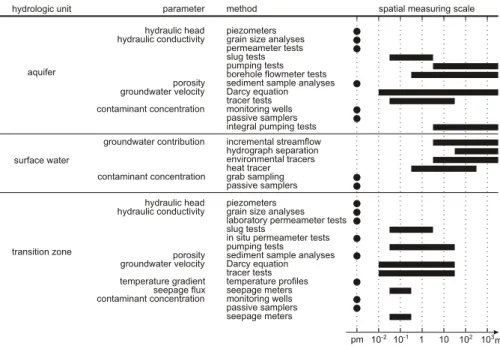
In general, apart from pumping tests, most methods applied in the subsurface pro-15

vide point estimates of the respective parameter, whereas most of the surface water methods represent larger sample volumes (Fig. 1). Measurements of hydraulic head, grain size analysis, and permeameter tests are point measurements. In slug and bail tests and tracer tests, the portion of sampled aquifer volume is larger, on the scale of meters around the sample point. Pumping tests operate on the largest scale among 20

the methods applied in the subsurface, typically on the scale of tens of meters up to kilometers. Measurements of the temperature gradient in the transition zone provide point estimates of flux. Seepage meter measurements yield flux estimates over the diameter of the seepage pan, usually less than one meter. Incremental streamflow measurements result in groundwater discharge estimates averaged over the reach 25

length between measurement transects, ranging from several meters to hundreds of meters. The same applies to environmental and heat tracer methods aiming at iden-tifying groundwater contribution to streamflow. Hydrograph separation delivers

(26)

HESSD

Full Screen / Esc

mation on the groundwater discharge upstream of a gauging station and, therefore, enables the calculation of discharge rates averaged over the upstream length. Con-cerning contaminant concentration, water sampling from piezometers or from surface water, passive samplers and seepage meters provide point measurements of contami-nant concentration, whereas integral pumping tests yield concentrations averaged over 5

a large aquifer volume.

The various methods also differ in the time scale they represent. The majority of techniques deliver parameter estimates at a certain point in time. Only seepage me-ters and passive samplers collect water volume and contaminant mass, respectively, over a time period from hours to weeks and, thus, yield time-averaged fluxes. Hy-10

drograph separation gives estimates of the groundwater contribution to streamflow av-eraged over the duration of the recorded hydrograph, typically from several years to decades. Automated sampling methods or data loggers, however, can help breaking down measurement time steps to intervals that allow for observations of temporal vari-ations. In particular, parameters that can be measured simply using probes, such as 15

pressure or temperature, are suitable for long-term monitoring. For instance, pressure transducers may be installed in piezometers to monitor variations in hydraulic head, or temperature probes may be buried in the subsurface to analyse diurnal to seasonal fluctuations.

For measurements conducted in heterogeneous media, such as the subsurface, the 20

measurement scale on which a selected technique operates may have a significant in-fluence on the results, which has clearly been demonstrated for hydraulic conductivity in numerous studies. As Rovey and Cherkauer (1995) point out, hydraulic conductivity generally increases with test radius, because with a larger test radius the chance to encounter high-conductivity zones in a heterogeneous medium increases. Schulze-25

Makuch and Cherkauer (1998) found that hydraulic conductivity estimates increased during individual aquifer tests as the volume of aquifer impacted increased. There-fore, they concluded that scale-dependency of hydraulic conductivity is not related to the measurement method, but to the existence of high-conductivity zones within

(27)

HESSD

Full Screen / Esc

a low-conductivity matrix. Schulze-Makuch et al. (1999) observed no scaling effects for homogeneous media, whereas for heterogeneous media they found an empirical rela-tion for the scaling behavior. The relarela-tionship is a funcrela-tion of the type of flow present (porous flow, fracture flow, conduit flow, double-porosity media) and the degree of het-erogeneity, associated with pore size and pore interconnectivity. The relationship was 5

found to be valid up to an upper boundary value, representing the scale above which a medium can be considered quasi-homogeneous. In many of the test results included in the study by Schulze-Makuch et al. (1999), hydraulic conductivities obtained by pump-ing tests were close to the upper boundary.

The scale-dependency of measurements in heterogeneous media implies that even 10

a dense grid of point measurements may deliver results that are considerably different from those obtained from larger-scale measurements, because the importance of small heterogeneities, such as narrow high-conductivity zones, may be underestimated. A better representation of the local conditions including the effects of scale on measure-ment results can be achieved by conducting measuremeasure-ments at multiple scales within a 15

single study site.

5.2 Groundwater discharge or hyporheic exchange flow

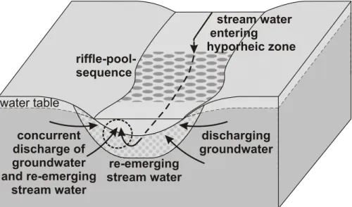
Exchange processes between streams and groundwater do not only comprise ground-water discharging to a stream or stream ground-water infiltrating into the aquifer, but also in-clude downwelling of stream water into the sediment and re-emerging to the stream 20

further downstream (Fig. 2). These small-scale exchange processes are driven by pressure variations caused by geomorphologic features such as pool-riffle sequences, discontinuities in slope, or obstacles on the streambed (Thibodeaux and Boyle, 1987; Savant et al., 1987; Hutchinson and Webster, 1998). This implies that water discharg-ing through the streambed into the stream can either be groundwater, or re-emergdischarg-ing 25

surface water, or a mixture of both. Harvey and Bencala (1993) found that the gross inflow (groundwater + subsurface flow) of water to their study stream exceeded the net inflow (groundwater only) by nearly twofold. Thus, methods to determine flux in

(28)

HESSD

Full Screen / Esc

the shallow streambed, such as seepage meters or shallow streambed piezometers, may result in discharge rates that may not necessarily be attributed to groundwater dis-charge. Qualitative methods, such as heat or environmental tracers, may also be used to elucidate the origin of the water. The retention of stream water in the streambed sediments has also been addressed by the transient storage model. Transient storage 5

refers to the temporary detainment of stream water in the sediment voids or in any other stagnant pockets of water, such as eddies or at the lee side of obstacles (Ben-cala and Walters, 1983). It is usually studied by injecting a conservative tracer into the stream and fitting a model to the tracer breakthrough curves which yields the deter-mination of storage zone size and exchange rate (Runkel, 1998). Numerous studies 10

have been conducted using stream tracers and the transient storage approach to char-acterize surface-subsurface water exchange (e.g., D’Angelo et al., 1993; Harvey and Bencala, 1993; Morrice et al., 1997; Hart et al., 1999). However, surface storage and hyporheic exchange are lumped together in this approach and the identification of the actual subsurface component is often difficult (Runkel et al., 2003).

15

5.3 Considerations for choosing appropriate methods

The study goal plays a decisive role for the choice of appropriate methods to character-ize groundwater – surface water interactions. The objective of the research project de-fines the required measurement scale which in turn constrains the possible methods. A regional assessment of water resources or the fate and transport of pollutants requires 20

information on a large scale, requiring methods that represent a large sample volume, such as pumping tests or surface water methods. Equally, if the impact of groundwater discharge on surface water quality or vice versa is of concern, measurements on a large scale may be more appropriate. In contrast, investigations of the spatial varia-tion of exchange processes and flow paths between groundwater and surface water 25

require measurements that allow for high spatial resolutions, such as temperature pro-files or piezometer methods. If temporal variations or trends are of concern, long-term monitoring of certain parameters may be required. Automated sampling methods and

(29)

HESSD

Full Screen / Esc

probes coupled with data loggers are most suitable for that purpose.

The choice between methods on a similar scale may be more of an operational character, considering factors such as accessibility of the study site, portability of the equipment, and financial and human resources, among others. Landon et al. (2001) compared instream methods for measuring hydraulic conductivity in sandy streambeds 5

(in situ permeameter tests, seepage meters coupled with hydraulic head measure-ments, slug tests, grain size distribution) and found that the spatial variability of hy-draulic conductivity was greater than the variability of hyhy-draulic conductivity between different methods. They concluded that the method used may matter less than making enough measurements to characterize spatial variability.

10

Uncertainties inherent in the different techniques may be taken into account when selecting methods to study groundwater – surface water interactions. Measurements of hydraulic conductivity are generally characterized by high uncertainties, because hy-draulic conductivity can vary over several orders of magnitude. Hence, flux estimates based on the Darcy equation are inherently inaccurate, which relates to the majority of 15

methods applied in the aquifer and the transition zone. Hydrograph separation is based on the assumptions that stream discharge can be directly correlated to groundwater recharge. Several factors are neglected in this approach, such as evapotranspiration and bank storage, leading to considerable uncertainties (Halford and Mayer, 2000). Tracer-based hydrograph separation further assumes that pre-event water and event 20

water are clearly different in isotopic or chemical composition and that the composition is constant in space and time; both being conditions that are often not met (Genereux and Hopper, 1998). Similarly, environmental and heat tracer measurements in the sur-face water rely on clearly pronounced and stable differences between groundwater and surface water, incorporating some degree of uncertainty. Flux estimates based on tem-25

perature gradients in the streambed are calculated on the assumption of vertical flow beneath the stream, which may not be true in the vicinity of the river banks or because of influences of hyporheic water movement as described before. Furthermore, the in-fluence of daily fluctuations in surface water temperature may create some error. Flux

(30)

HESSD

Full Screen / Esc

measurements made by conventional seepage meters may be influenced by the resis-tance of the collection system to streamflow (Murdoch and Kelly, 2003). The accuracy of contaminant concentrations from water samples is influenced by the handling of the samples and the detection sensitivity of the analysis methods. Passive flux meter mea-surements may further be affected by competitive sorption or rate-limited sorption, and 5

by fluctuations in flow direction in case of long-term measurements. The evaluation of integral pumping tests requires information on aquifer properties which may already be uncertain. In conclusion, inaccuracies are inherent in all methods to determine inter-actions between groundwater and surface water, so that an analysis of uncertainties along with any measurement is indispensable.

10

Because of the limitations and uncertainties associated with the various methods, any attempt to characterize stream-aquifer interactions may benefit from a multi-scale approach combining multiple techniques. For instance, flux measurements in the tran-sition zone alone may not suffice to clearly identify the groundwater component, while isotope concentrations alone may also lead to misinterpretations. Also, integrating 15

point measurements may not be a valid substitute for measurements on a larger scale due to the scale-effects of measurements in heterogeneous media. Therefore, mea-surements on multiple scales are recommended to characterize the various processes and include different factors controlling groundwater-surface water exchange. Further-more, a combination of measurements of physical and chemical properties may help 20

identify water sources and subsurface flow paths. For instance, Becker et al. (2004) combined current meter measurements with a stream temperature survey to both iden-tify zones of groundwater discharge and calculate groundwater inflow to the stream; Constantz (1998) analysed diurnal variations in streamflow and stream temperature time series of four alpine streams to quantify interactions between stream and ground-25

water; James et al. (2000) combined temperature and the isotopes of O, H, C, and no-ble gases to understand the pattern of groundwater flow; Harvey and Bencala (1993) used hydraulic head measurements and solute tracers injected into the stream and the subsurface to identify flow paths between stream channel and aquifer and to calculate

(31)

HESSD

Full Screen / Esc

exchange rates; Storey et al. (2003) used hydraulic head measurements, salt tracers injected into the subsurface, and temperature measurements in the stream and sub-surface to trace the flow paths in the hyporheic zone; Ladouche et al. (2001) combined hydrological data, geochemical and isotopic tracers to identify the components and ori-gin of stream water. An elaborate combination of methods can considerably reduce 5

uncertainties and constrain flux estimates.

6 Summary

Measuring interactions between groundwater and surface water is an important com-ponent for integrated river basin management. Numerous methods exist to measure these interactions which are either applied in the aquifer, in the surface water, or in the 10

transition zone itself.

The methods differ in resolution, sampled volume, and the time scales they repre-sent. Often, the choice of methods constitutes a trade-off between resolution of hetero-geneities and sampled subsurface volume. Furthermore, the measurement scale on which a selected technique operates may have a significant influence on the results, 15

leading to differences between estimates obtained from a grid of point measurements and estimates obtained from large-scale techniques. Therefore, a better representa-tion of the local condirepresenta-tions including the effects of scale on measurement results can be achieved by conducting measurements at multiple scales at a single study site.

Attention should be paid to distinguish between groundwater discharge and hy-20

porheic exchange flow. Small-scale flow measurements in the shallow streambed may not suffice to make this distinction, so that additional measurements to identify the water source are recommended.

The study goal plays a decisive role in choosing appropriate methods. For regional investigations large-scale techniques may be more suitable, whereas process studies 25

may require measurements which enable high resolution. All methods have their lim-itations and uncertainties. However, a multi-scale approach combining multiple

(32)

HESSD

Full Screen / Esc

niques can considerably reduce uncertainties and constrain estimates of fluxes be-tween groundwater and surface water.

Acknowledgements. This work was supported by the European Union FP6 Integrated Project

AquaTerra (Project no. 505428) under the thematic priority “sustainable development, global change and ecosystems”.

5

References

Alyamani, M. S. and Sen, Z.: Determination of Hydraulic Conductivity from Complete Grain-Size Distribution Curves, Ground Water, 31(4), 551–555, 1993.

Anderson, M. P.: Heat as a ground water tracer, Ground Water, 43(6), 951–968, 2005.

Arnold, J. G., Allen, P. M., Muttiah, R., and Bernhardt, G.: Automated Base-Flow Separation

10

and Recession Analysis Techniques, Ground Water, 33(6), 1010–1018, 1995.

Barnes, B. S.: The structure of discharge recession curves, Trans. Am. Geophys. Union, 20, 721–725, 1939.

Bauer, S., Bayer-Raich, M., Holder, T., Kolesar, C., M ¨uller, D., and Ptak, T.: Quantification of groundwater contamination in an urban area using integral pumping tests, J. Contam.

15

Hydrol., 75, 183–213, 2004.

Baxter, C., Hauer, F. R., and Woessner, W. W.: Measuring groundwater-stream water ex-change: New techniques for installing minipiezometers and estimating hydraulic conductivity, Trans. Am. Fisher. Society, 132(3), 493–502, 2003.

Bayer-Raich, M., Jarsj ¨o, R., Liedl, R., Ptak, T., and Teutsch, G.: Average contaminant

con-20

centration and mass flow in aquifers from time-dependent pumping well data: Analytical framework, Water Resour. Res., 40, W08303, doi:10.1029/2004WR003095, 2004.

Becker, M. W., Georgian, T., Ambrose, H., Siniscalchi, J., and Fredrick, K.: Estimating flow and flux of ground water discharge using water temperature and velocity, J. Hydrol., 296(1–4), 221–233, 2004.

25

Bencala, K. E. and Walters, R. A.: Simulation of Solute Transport in a Mountain Pool-and-Riffle Stream: A Transient Storage Model, Water Resour. Res., 19(3), 718–724, 1983.

Beyer, W.: Zur Bestimmung der Wasserdurchl ¨assigkeit von Kiesen und Sanden aus der Korn-verteilungskurve, Wasserwirtschaft Wassertechnik, 14(6), 165–168, 1964.