HAL Id: hal-00302757
https://hal.archives-ouvertes.fr/hal-00302757
Submitted on 1 Aug 2006
HAL is a multi-disciplinary open access
archive for the deposit and dissemination of
sci-entific research documents, whether they are
pub-lished or not. The documents may come from
teaching and research institutions in France or
abroad, or from public or private research centers.
L’archive ouverte pluridisciplinaire HAL, est
destinée au dépôt et à la diffusion de documents
scientifiques de niveau recherche, publiés ou non,
émanant des établissements d’enseignement et de
recherche français ou étrangers, des laboratoires
publics ou privés.
scintillation
M. Tokumaru, M. Kojima, K. Fujiki, M. Yamashita
To cite this version:
M. Tokumaru, M. Kojima, K. Fujiki, M. Yamashita. Tracking heliospheric disturbances by
interplan-etary scintillation. Nonlinear Processes in Geophysics, European Geosciences Union (EGU), 2006, 13
(3), pp.329-338. �hal-00302757�
Nonlin. Processes Geophys., 13, 329–338, 2006 www.nonlin-processes-geophys.net/13/329/2006/ © Author(s) 2006. This work is licensed
under a Creative Commons License.
Nonlinear Processes
in Geophysics
Tracking heliospheric disturbances by interplanetary scintillation
M. Tokumaru, M. Kojima, K. Fujiki, and M. Yamashita
Solar-Terrestrial Environment Laboratory, Nagoya University, Toyokawa, Aichi 442-8507, Japan Received: 18 January 2006 – Revised: 8 May 2006 – Accepted: 8 May 2006 – Published: 1 August 2006
Abstract. Coronal mass ejections are known as a solar cause
of significant geospace disturbances, and a fuller elucida-tion of their physical properties and propagaelucida-tion dynamics is needed for space weather predictions. The scintillation of cosmic radio sources caused by turbulence in the solar wind (interplanetary scintillation; IPS) serves as an effec-tive ground-based method for monitoring disturbances in the heliosphere. We studied global properties of transient so-lar wind streams driven by CMEs using 327-MHz IPS ob-servations of the Solar-Terrestrial Environment Laboratory (STEL) of Nagoya University. In this study, we reconstructed three-dimensional features of the interplanetary (IP) counter-part of the CME from the IPS data by applying the model fitting technique. As a result, loop-shaped density enhance-ments were deduced for some CME events, whereas shell-shaped high-density regions were observed for the other events. In addition, CME speeds were found to evolve sig-nificantly during the propagation between the corona and 1 AU.
1 Introduction
The Sun emits a continuous supersonic stream of plasma called the solar wind. The solar wind produces the helio-sphere, which is a huge bubble in space, extending well be-yond the orbit of Pluto. Thus, this supersonic flow engulfs all planets of the solar system, and interacts with them. In the case of the Earth, the solar wind is blocked and deflected by its intrinsic magnetic field, and the magnetosphere is shaped through this interaction.
The large-scale structure of the highly variable solar wind changes drastically over the course of the well-known 11-year sunspot cycle. In addition, transient disturbances of Correspondence to: M. Tokumaru
the solar wind are sometimes generated by eruptive phe-nomena in the solar atmosphere. These solar wind varia-tions affect the space environment around the planets, and they sometimes cause significant disturbances in the mag-netosphere or upper atmosphere of the Earth. Such space disturbances cause adverse conditions for space-borne sys-tems and astronauts. In the worst case, spacecraft are lost due to unrecoverable failures, and human health is endan-gered. Thus, solar-driven disturbances are a serious threat for human advances into space. Ground-based technologi-cal systems such as radio communications, power facilities, navigations, which are fundamental services for our life, are also vulnerable to space disturbances. In order to minimize the loss of space-borne or ground-based systems, a precise prediction of the time-variable conditions in the space envi-ronment (so-called “space weather prediction”) is needed in the near future (Marubashi, 1989; Luhmann, 1997).
Among various kinds of solar activities, coronal mass ejec-tions (CMEs) are known to cause significant space distur-bances (Gosling, 1993; Lindsay et al., 1995). In this sense, CMEs are the primary targets for space weather predictions (Luhmann, 1997). A CME is a sudden release of dense plasma and strong magnetic flux into interplanetary space. It is usually identified from coronagraphic observations as a transient bright feature moving outward from the sun. Typ-ical values of mass and energy for a single CME event are 1015–1016g and 1030–1031 erg, respectively (St. Cyr et al., 2000; Yashiro et al., 2004). CME speeds range from several 10s km/s to >2000 km/s, and the mean value is ∼450 km/s (St. Cyr et al., 2000; Yashiro et al., 2004). It should be noted here that these are projected speeds. Fast CMEs drive shock waves in the solar wind, and CME-driven shocks acceler-ate energetic particles (Reames, 1999), which are hazardous for spacecraft instruments and astronauts. When CMEs im-pact the Earth’s magnetosphere, they can give rise to geo-magnetic disturbances (Lindsay et al., 1995; St. Cyr et al., 2000), which can have detrimental effects on space-borne
(a) (b)
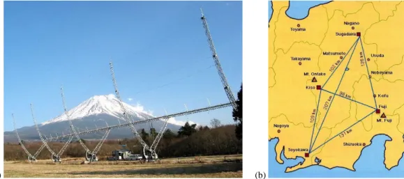
Fig. 1. (a) The 327-MHz radiotelescope at Fuji Observatory, and (b) geographic locations of STEL four-station system.
and ground-based systems via energetic particles and fluc-tuating magnetic fields.
The 3-dimensional structure and propagation dynamics of CME are the fundamental knowledge required to predict space weather from observational data near the Sun. How-ever, they are poorly understood owing to the lack of observa-tional data. In particular, CME observations in the solar wind are rather sparse, and the global properties of CME between the Sun and the Earth orbit are still largely obscure. We have been addressing this problem with observations of inter-planetary scintillation (IPS; Tokumaru et al., 2000, 2003a, b, 2005a, b, c). IPS serves as an effective ground-based method to observe the solar wind (e.g. Hewish et al., 1964; Hewish, 1989). IPS observations are particularly useful to study the global properties of transient streams associated with CMEs, since they allow us to probe a large volume of the inner he-liosphere in a short time (Gapper et al., 1982; Watanabe and Schwenn, 1989).
This paper reports recent results from our IPS study of CMEs. The outline of this paper is as follows. In Sect. 2, we describe solar wind observations made with the 327-MHz IPS system of the Solar-Terrestrial Environment Laboratory (STEL) of Nagoya University. In Sect. 3, we describe an analysis used to retrieve the 3-dimensional distribution of a CME from our IPS data. In Sect. 4, we present some results obtained from our IPS observations. In Sect. 5, we summa-rize and discuss the results.
2 Interplanetary scintillation measurements of the solar wind
Since the solar wind is a turbulent medium, small-scale den-sity irregularities are ubiquitous in the heliosphere. Radio waves from cosmic sources are scattered by these density ir-regularities, and rapid fluctuations of the signal intensity are observed on the ground. This phenomenon is called
inter-planetary scintillation, in short IPS (Hewish et al., 1964). IPS has been employed as a useful remote-sensing probe for the solar wind plasma since its discovery. We can derive a bulk flow speed of the solar wind by detecting a time difference between the IPS diffraction patterns observed at two sepa-rated stations (Dennison and Hewish, 1967). We can also estimate solar wind density fluctuation levels along a line-of-sight from observed IPS strength, if wave scattering is weak (Hewish and Symonds, 1969). In addition, power spectra of IPS provide information on the solar wind density turbulence (Readhead et al., 1978).
If we observe IPS for many radio sources in a day, we can produce a sky projection map of the solar wind on a daily ba-sis. Such mapping observations by IPS are quite suitable for detecting and tracking solar wind disturbances between the Sun and the Earth orbit. This unique IPS capability was first demonstrated by observations with the Cambridge 36 000 m2 array at a frequency of 81.5 MHz (Gapper et al., 1982). Al-though IPS observations there have been discontinued, the utility of IPS mapping observations for studying IP distur-bances has been demonstrated by research groups in Rus-sia (Vlasov, 1979), India (Manoharan et al., 2001) and Japan (Tokumaru et al., 2000). These IPS facilities use higher fre-quencies, enabling observations closer to the Sun.
Our IPS observations have been carried out regularly since the early 1980s using the 327-MHz multi-station system (Ko-jima and Kakinuma, 1990; Asai et al., 1995). Figure 1 shows the geographic location of the STEL IPS system and one of the IPS antennas (the 327-MHz radio-telescope at Fuji Observatory). Each IPS antenna has a large collecting area (∼2000 m2) to detect faint signals from weak sources. The available scintillation sources changes as the Sun moves against the background from day to day and those with so-lar elongation less than 90◦are selected for observation. In our IPS observations, 30–40 sources are observed daily be-tween April and December of every year. IPS observations
M. Tokumaru et al.: Tracking heliospheric disturbances by IPS 331
(a) (b)
Fig. 2. (a) SOHO/LASCO image for the CME event on 10 July 2000 (from http://lasco-www.nrl.navy.mil/), and (b) sky-projection map of
g-value obtained from our IPS observations between 11 July 2000, 22:00 UT and 12 July 2000, 07:00 UT. The center of the g-value map corresponds to the location of the Sun, and dotted concentric circles are constant RSEsinε (AU) contours drawn every 0.3 AU, where ε is the
solar elongation angle and RSE∼1 AU. Circles indicate line-of-sight locations where g-values were measured, and size and color represent the strength of g-value.
are not conducted during the months January to March owing to heavy annual snowfall in the mountainous regions where the IPS antennas are located. Solar wind speeds and scintil-lation levels are derived from our IPS observations.
We show an example of our IPS observations for a CME event in Fig. 2. A white-light image of a CME observed by the LASCO C3 coronagraph (Bruecker et al., 1995) is shown in the left panel of Fig. 2. As shown here, a bright CME was observed on the northeast limb on 10 July 2000. The right panel of Fig. 2 is a sky projection map produced from our IPS observations between 11 and 12 July 2000. The center of this map corresponds to the location of the Sun, and the dotted circles are constant R(≡RSEsinε) contours drawn
ev-ery 0.3 AU (where RSEand ε are the Sun-Earth distance and
the solar elongation angle, respectively). In this map, den-sity disturbance factors, so-called g-values (Gapper et al., 1982), derived from our IPS observations are indicated by circles. Color and size of the circles represent the strength of g-values. The g-value is a measure of the scintillation level for a line-of-sight of a given source, and is related to solar wind density fluctuations 1Ne integrated along the
line-of-sight when wave scattering is weak. Note that the small-scale turbulence level of 1Ne is roughly proportional to the
so-lar wind electron density Ne (Armstrong and Coles, 1978):
Ne∝1Ne. In the case of 327-MHz, the weak scattering
con-dition holds for R>0.2 AU, where R is the radial distance from the Sun. The g-value is normalized to the turbulence level of the quiet solar wind, so that g>1 means an excess of
1Ne. When enhanced density fluctuations associated with
CMEs intersect a line-of-sight, we obtain an abrupt increase in g-value. As shown in Fig. 2, marked enhancements in
g-value were observed at radial distances between 0.4 and 0.6 AU in the northeast quadrant about one day after the oc-currence of the CME event in the corona. These g-value enhancements are considered as an interplanetary counter-part of the 10 July 2000 CME event. It should be noted that the distribution of enhanced g-values in the map is in good agreement with the radial extension of brightness enhance-ments in the LASCO image. Accompanying the g-value en-hancements were distinct increases in the solar wind speeds derived from our IPS observations.
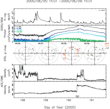
We show another example of CME observations made with the STEL IPS system in Fig. 3. Sky projection g-value maps produced from our IPS observations for 4 consecutive days (between 5 and 9 June 2000) are indicated in the mid-dle panel of Fig. 3. The upper two panels show solar soft X-ray intensity and energetic proton fluxes measured by the GOES geosynchronous satellite, and the lower two panels show the solar wind density and speed measured by the ACE spacecraft at the L1 point (McComas et al., 1998). A fast CME event occurred on 6 June 2000, in association with an X2.3/3B flare and a solar proton event. This CME event ex-hibited a circular shape of a bright material surrounding the Sun and propagating outward in all directions. Such an event, which is called a halo CME, is interpreted as a CME directed to the Earth. An IP shock driven by this halo CME was ob-served by ACE on 8 June 2000 at 09:00 UT. As shown in Fig. 3, clear increases in the g-values, ascribed to an IP dis-turbance associated with the halo CME, were observed on 7–9 June several hours before the arrival of the IP shock at ACE. Solar wind velocity increases (from ∼400 km/s to
∼600 km/s) were also detected from our IPS observations
Fig. 3. (From top to bottom) Solar soft X-ray flux and ener-getic (>1, >5, >10, and >30 MeV) proton flux observed by the GOES-8 satellite (from http://spidr.ngdc.noaa.gov), sky-projection g-value maps produced from STEL IPS observations, solar wind density and speed measured by ACE spacecraft (from http://www. srl.caltech.edu/ACE/ASC/level2/index.html) for the period between 5 June 2000, 15:00 UT and 9 June 2000, 15:00 UT. The onset of an SSC (sudden storm commencement) is indicated in the bottom panel.
during the same period. This velocity jump is smaller than that associated with the IP shock, however it is not incon-sistent with the ACE observations since IPS speeds include the effect of line-of-sight (LOS) integration. An important point to note on our IPS data is that enhanced g-values form a ring-shaped distribution encircling the Sun in the map. This feature is consistent with the fact that the event was Earth-directed.
The IPS sky projection maps thus reveal information on the 3-dimensional properties (e.g. radial distance, angular ex-tent, propagation direction) of the CME in the solar wind. However, attention must be paid to the inherent line-of-sight (LOS) integration in IPS observations, which can signifi-cantly affect the apparent features. Therefore, we need to remove the integration effect carefully in order to elucidate the CME’s 3-dimensional properties in more detail.
3 Model fitting analysis of IPS observations
We fit a 3-dimensional model of the solar wind, which in-cludes a transient component, to our IPS observations in or-der to remove the LOS integration effect. We briefly describe the method here (a detailed description is presented in
Toku-maru et al., 2003a). In this analysis, we exclusively used g-value data derived from our IPS observations, since an an-alytical method to deconvolve the solar wind velocity data of transient events is not yet available.
For weak scattering, the g-value is given by the following equation g2= 1 K Z ∞ 0 1Ne2w(z)dz, (1) where z is a distance along the line-of-sight, and w(z) is the IPS weighting function (Young, 1971) which is given by
w(z) = Z ∞ 0 k1−qsin2 k 2zλ RF 4π ! exp −k 2z292 2 ! dk.(2)
Here, k, q, λRF, and 9 are the spatial wavenumber and the
spectral index of density turbulence, the wavelength for the observing frequency (0.92 m for 327 MHz), and the apparent angular size of the radio source, respectively. The intrinsic value of 9 is different for each source, however accurate in-formation on it is unavailable for all sources used in our IPS observations. Therefore, we assumed here 9=0.1 arcsec-ond, which is a typical value of a scintillation source at 327 MHz. Note that more realistic values of 9 would not produce any significant changes in the analysis, since model calcu-lations of the g-value are insensitive to 9. The solar wind turbulence is known to be well described by the Kolmogorov spectrum (q=11/3) for all distances except for the vicinity of the Sun (Woo and Armstrong, 1979). Therefore, we assumed
q=11/3 in the analysis. We also assumed 1Ne=fNe1Ne0, where 1Ne0, fNe are the density fluctuation level of the am-bient solar wind and a dimensionless parameter to represent the deviation (either excess or deficit) from the ambient level, respectively. In Eq. (1), K is a normalization factor, which is given by K≡R∞
0 1N 2
e0w(z)dz.
Provided that a suitable model for the 3-dimensional dis-tribution of 1Nein the solar wind is given, the g-value can
be calculated by using Eqs. (1) and (2). This fact enables us to determine a realistic 1Ne model by comparing between
calculated and observed g-values. The basic idea to provide observational constraints on a model of IP disturbances by using g-value data was first proposed by Tappin (1987). In his study, a shell-shaped 1Neenhancement model which
as-sumed an isotropic angular extent was used. The 1Nemodel
fit to our g-value data is similar to the one used by Tappin (1987), but with some distinct differences. For example, our
1Ne model allows for anisotropy of the angular extent and
angular dependence of the propagation speed, thereby more closely simulating the global features of an enhanced 1Ne
region.
To fit IPS data for CME events, we employed a 1Ne
model, which included a localized enhancement (fNe) above an isotropic radial gradient of the background level (1Ne0).
In our analysis, the 1Ne enhanced region was assumed to
M. Tokumaru et al.: Tracking heliospheric disturbances by IPS 333 e-folding radial thickness D, an e-folding major angular
ex-tent θ0, a ratio of minor-to-major angular extent AR, an
in-clination of the maximum angular elongation β (defined in the plane of sky in a counterclockwise sense), a peak value
C1, and the heliographic coordinates of the central axis (λ0, φ0). For small D and AR∼1, our model represents a shell
or bubble-shaped CME structure, and AR<1 means an elon-gated structure in a direction defined by β. The 1Ne
en-hanced region was also assumed to expand radially at a given speed VSduring IPS observations. It has been reported from
earlier studies that the maximum expansion speed of an IP shock or disturbance is likely to occur in the radial direction above the flare site (Smart and Shea, 1985). In this analy-sis, we use the following function to account for the angular dependence of the expansion speed
VS =VS0cosα(θ/2), (3)
where α and θ are the index of curvature and the separation angle with respect to the center axis of the 1Neenhanced
re-gion, respectively. As for the background component, 1Ne0
is assumed to be distributed as R−2, and this is validated by many observational studies (e.g. Hewish and Symonds, 1969; Armstrong and Coles, 1978).
We calculated the g-values with Eqs. (1) and (2) and the
1Ne model by considering the geometry of IPS
observa-tions for a given day, and optimized the model to measured g-values by adjusting nine parameters: D, θ0, AR, β, C1, λ0, φ0, VS0, and α. The optimization was done by minimizing
the rms deviation σ given by
σ2= 1 N N X i=1 (gobs−gcal)2 g2obs (4)
where gobsand gcalare the observed and calculated g-values,
respectively, and N is the number of observations. We used the Simplex method to search for the minimum. The Simplex method is an effective minimizing algorithm for general non-linear functions without using derivatives, and it attempts to enclose the minimum inside an irregular volume defined by a “simplex” (i.e. a polyhedron in n-dimensional space, one dimension for each parameter defining the model). The sim-plex size is continuously changed and mostly diminished so that finally it is small enough to contain the minimum with the desired accuracy. The convergence criterion used in the analysis is that the change in σ2at each iteration is within a fractional tolerance level of 10−6. A few hundred iterations
are typically needed for convergence.
The sharpness of the σ2 variation around the minimum can be used as a measure of the estimation error for a given parameter. The estimation errors in the analysis depend on the observation geometry (the heliocentric distance and the propagation direction of CMEs) as well as goodness of the fit. In the case of IPS observations of an Earth-directed CME at distances 0.5–0.8 AU (the most frequent case in this anal-ysis, see the next section), the coordinate of the central axis
(λ0, φ0) and the angular extent anisotropy AR are best
de-termined among the model parameters. Typical values of the estimation errors for the coordinates and AR are ∼5◦ and
∼0.01, respectively, as far as a high degree of the correla-tion is obtained. In comparison, estimacorrela-tion of the inclinacorrela-tion angle β is somewhat crude, with typical errors being 5−10◦. The estimation errors of these parameters, particularly that of longitude, increase with increasing separation angle between the central axis and the Sun-Earth line. Note that AR and β are hardly determined for the case of broadside observation geometry. The estimation errors of the propagation speed
VS0 are usually small, typically a few % even for the halo
geometry. On the other hand, the halo geometry is not suit-able to obtain relisuit-able estimates of the angular extent θ0and
the enhancement factor C1, since these parameters are
cou-pled. Typical values of the estimation error for θ0and C1are
10−20◦and ∼30%, respectively, for the halo geometry. The
estimation errors of the radial thickness D are typically 0.01– 0.03 AU. The estimates of the curvature index α are usually associated with large errors, ∼0.5, although this parameter is essential to obtain a good fit for some events.
As mentioned above, the model used here is a rather sim-ple one which assumes a smooth variation with a single peak. It is obvious that the current version of the model fitting anal-ysis can not deal with IPS data which include either irregular structures or multiple components of IP disturbances. Nev-ertheless, we think that this analysis is useful to determine large-scale properties of an isolated CME event.
4 Results
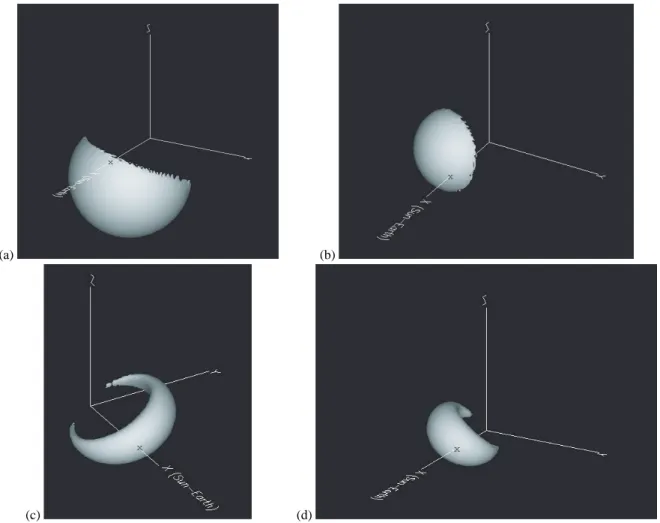
Remote-observer views of the best fit model for some CME events are displayed in Fig. 4. Detailed descriptions of the analysis for these CME events are presented in Tokumaru et al. (2003a, b, 2005b, c). An iso-1Necounter of the
enhance-ment component for a given level is plotted here. It should be noted that the R−2 gradient of the background compo-nent is removed in this figure. The origin of each plot corre-sponds to the location of the Sun, and the x-axis is directed to the Earth. The length of each axis represents 1 AU. These models are thought as a first-order approximation of global features of CMEs in the solar wind, and they are found to be generally consistent with white-light or in situ measure-ments of CMEs, as discussed in other studies (Tokumaru et al., 2003a, b, 2005b, c). An important point to note is that there is a variety of the angular extent; some of CME events had an elongated structure (AR<1), and some had a shell-shaped structure with a nearly isotropic angular extent (AR∼1). This aspect of interplanetary CMEs was not fully appreciated from earlier observational studies. An accurate description of the global morphology is clearly essential for improving space weather predictions.
We have analyzed our IPS data for 16 CME events in-cluding those shown in Fig. 4. The analyzed CME events
(a) X (b) X (c) X (d) X
Fig. 4. Remote-observer’s views of the best fit model determined for (a) 20 September 1999, (b) 10 July 2000, (c) 14 July 2000 (adopted
from Tokumaru et al., 2003a), and (d) 28 October 2003 CME events. The solar ecliptic coordinate system is used here, and the xy-plane is the ecliptic. The heliographic coordinates of the central axis for (a–d) are S35E04, N13E21, N11W17, and N15E15, respectively. The intersection point of the outer shell/loop of the IP disturbance with the x-axis is marked by a cross in each panel.
occurred between 1998 and 2003, and they were selected by the following two criteria; (1) g-value enhancements with
g>1.5 were observed for several lines-of-sight in associa-tion with the occurrence of a CME observed with LASCO. Since no LASCO observations were available during July– September in 1998, we identified the CME occurrence from in situ observations of the magnetic flux rope at 1 AU dur-ing this period. Most of the events selected here were as-sociated with halo or partial halo CMEs. This is attributed to the fact that our IPS observations have greater sensitivity for Earth-directed CMEs than those over the limb. Strictly speaking, CMEs propagating in an oblique direction with re-spect to the Sun-Earth line are best observed by IPS, and the maximum sensitivity for a given direction depends on the ra-dial distance. (2) A significant correlation between observed and calculated g-values was obtained by the analysis: i.e. correlation coefficients ρ>0.5. Since the model fitted to ob-servations is rather simple, many CME events with a more complex structure were excluded by this criterion.
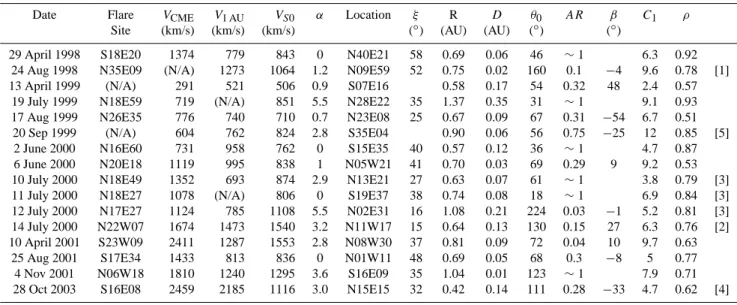
The best fit parameters VS0, α, λ0, φ0, D, θ0, AR, β, C1
determined for these CME events are listed in Table 1. The parameters R and ρ in the table correspond to heliocentric distances of 1Nepeak and correlation coefficients between
observed and calculated g-values, respectively. The latter is a measure of goodness of the fit, and used to select the CME events, as mentioned above. Heliographic locations of as-sociated flare, separation angles between the flare site and the central axis ξ , plane-of-sky speeds of CME measured by LASCO VCME, and the average Sun-Earth transit speeds V1 AUare also shown in the table. The VCMEdata were taken
from the SOHO/LASCO CME catalog (Yashiro et al., 2004), and the V1 AUdata were determined from the time difference
between the CME occurrence and the IP shock arrival at 1 AU. Mean values of VCMEand V1 AU for all events were
1264 km/s and 1036 km/s, respectively. Thus, high-speed events were selected in this study. This selection bias may come from the fact that fast CME events can effectively give rise to 1Neenhancements in the solar wind.
M. Tokumaru et al.: Tracking heliospheric disturbances by IPS 335 Typical features of interplanetary CMEs deduced from the
analysis results are summarized below. Here, one must be reminded of a bias due to the event selection effect.
– An elongated (AR<0.35) structure was determined for
about 60% of analyzed events. The major angular span of the elongated structure was about 4 times (on an av-erage) greater than that of the minor one. The structure tended to elongate in the longitudinal direction, while a large inclination (|β|>45◦) was observed for some CME events that occurred in 1999. For the isotropic events, a mean value of the angular span was about 50◦.
– The radial thickness was small, D∼0.1 AU, and there
was no significant difference in D between elongated and isotropic events. This thickness is consistent with a typical size of the IP shock thickness at 1 AU (Borrini et al., 1982).
– The mean value of the peak enhancement factor was
about 7 for all analyzed events, and no significant differ-ence was found between elongated and isotropic events. Provided that Ne∝1Neand the ambient solar wind
den-sity is ∼5/cc at 1 AU, this peak enhancement factor cor-responds to ∼35/cc.
– The central axis of the best fit model (λ0, φ0) differed
significantly from that of the associated flare site for some events, and an mean angular separation between the flare site and the inferred central axis is 36◦, larger than the estimation errors. This means that the center of an interplanetary CME does not necessarily lie above the flare site. No systematic shift was found in either longitude or latitude.
– The propagation speeds VS0 showed large diversity,
ranging between ∼500 km/s and > 1500 km/s (aver-age ∼970 km/s). When these speed data are compared with VCME and V1 AU, some CMEs are found to
de-celerate significantly during propagation. Other CMEs show insignificant change of propagation speed or some acceleration between the Sun and the Earth orbit.
– A mean value of α was about 2, although derived values
ranged between 0 and 5.5, and this is in excellent agree-ment with the empirical model (α=2) derived from a statistical study of IP shocks (Smart and Shea, 1985). There was no significant difference between elongated and isotropic events.
5 Summary and discussion
STEL IPS observations were analyzed to study the global features of interplanetary CMEs, which is one of the pieces of key information needed to improve space weather predic-tions. We reconstructed the 3-dimensional distribution of
CME-generated 1Ne enhancements in the solar wind from
our g-value data by using the model fitting method. As a re-sult, we successfully fit a 3-dimensional model of 1Ne
dis-tribution to our IPS observations for 16 selected CME events for the period 1998 to 2003. Some of the best fit models sug-gested that the CMEs were elongated in a given direction, be-ing loop-shaped. Other models suggested that the CMEs had shell-shaped distribution with a nearly isotropic angular ex-tent. The maximum angular extent of the elongated structure tended to occur in a longitudinal direction, while large incli-nations (>45◦) were observed for the CME events in 1999. The radial thickness of the model density enhancement was usually small, and generally consistent with a typical scale of the density compression region associated with IP shocks at 1 AU. Evolution of CME propagation speeds in the so-lar wind was also disclosed by comparing our IPS observa-tions with coronal and/or near-Earth observaobserva-tions. Some of the data suggested that the CMEs were significantly deceler-ated during propagation between the Sun and the Earth orbit. Other data indicated that the CMEs propagated at an almost constant speed, or gradually accelerated during propagation. The mean value of α, which controls the angular dependence of the propagation speed, was found to be nearly equal to the one used in the empirical model of the IP shock, although measured α showed a large scatter.
Following earlier studies (e.g. Watanabe and Schwenn, 1989; Moore and Harrison, 1994; Manoharan et al., 2001), we used 1Neenhancements observed by IPS as a proxy for
interplanetary CMEs. However, we should keep in mind that the origin of 1Ne enhancements is still an unsettled
ques-tion. That is, there are two possible interpretations for 1Ne
enhancements; one is the shocked solar wind plasma (i.e. the energized ambient solar wind) and the other is a core plas-moid of coronal origin (so called “coronal ejecta”). IPS ob-servations cannot discriminate between these two unless one carefully examines their correspondence with other comple-mentary observations for a CME event.
It was reported from a comparison study using Cam-bridge IPS observations and in situ data that a majority of g-value enhancements were associated with the compres-sion region between the transient high-speed flow and the IP shock driven by a CME (Moore and Harrison, 1994). The global features revealed from our IPS observations are found to be generally consistent with characteristics of the shocked plasma for most of the cases. In particular, the shell-shaped 1Ne-enhanced regions are well explained by a
high-density plasma generated at the shock front through interac-tion between a fast CME and a nearly uniform ambient so-lar wind. The loop-like density-enhanced structure also can be explained by the shocked plasma provided that the ambi-ent solar wind structure is bimodal. The solar wind is com-posed of fast and slow speed components, and the shocked plasma is expected to develop predominantly in the slow wind, since strong compression takes place there. There-fore, an elongated structure of 1Ne enhancements is likely
Table 1. Model parameters for 16 CME events. VS0, α, coordinate of the center axis (longitude and latitude), D, θ0, AR, β, C1and
correlation coefficients ρ determined from the g-value data are shown. Heliographic locations of the associated flare, angular separations between the flare site and the central axis ξ , heliocentric distances R are also shown in this table. The dates of CME occurrence are used except for the cases of 24 August and 23 September 1998 events when coronagraph observations by the SOHO spacecraft were unavailable. Instead, flare occurrence dates are used for these cases. Plane-of-sky speeds of CME VCME (from http://cdaw.gsfc.nasa.gov/CME list/
index.html), heliographic coordinates of associated flare site, and Sun-Earth transit speeds of IP shock V1 AUare included in this table for
comparison. See [1] Tokumaru et al. (2000), [2] Tokumaru et al. (2003a), [3] Tokumaru et al. (2003b), [4] Tokumaru et al. (2005b), [5] Tokumaru et al. (2005c).
Date Flare VCME V1 AU VS0 α Location ξ R D θ0 AR β C1 ρ
Site (km/s) (km/s) (km/s) (◦) (AU) (AU) (◦) (◦)
29 April 1998 S18E20 1374 779 843 0 N40E21 58 0.69 0.06 46 ∼1 6.3 0.92
24 Aug 1998 N35E09 (N/A) 1273 1064 1.2 N09E59 52 0.75 0.02 160 0.1 −4 9.6 0.78 [1]
13 April 1999 (N/A) 291 521 506 0.9 S07E16 0.58 0.17 54 0.32 48 2.4 0.57
19 July 1999 N18E59 719 (N/A) 851 5.5 N28E22 35 1.37 0.35 31 ∼1 9.1 0.93
17 Aug 1999 N26E35 776 740 710 0.7 N23E08 25 0.67 0.09 67 0.31 −54 6.7 0.51
20 Sep 1999 (N/A) 604 762 824 2.8 S35E04 0.90 0.06 56 0.75 −25 12 0.85 [5]
2 June 2000 N16E60 731 958 762 0 S15E35 40 0.57 0.12 36 ∼1 4.7 0.87
6 June 2000 N20E18 1119 995 838 1 N05W21 41 0.70 0.03 69 0.29 9 9.2 0.53
10 July 2000 N18E49 1352 693 874 2.9 N13E21 27 0.63 0.07 61 ∼1 3.8 0.79 [3]
11 July 2000 N18E27 1078 (N/A) 806 0 S19E37 38 0.74 0.08 18 ∼1 6.9 0.84 [3]
12 July 2000 N17E27 1124 785 1108 5.5 N02E31 16 1.08 0.21 224 0.03 −1 5.2 0.81 [3]
14 July 2000 N22W07 1674 1473 1540 3.2 N11W17 15 0.64 0.13 130 0.15 27 6.3 0.76 [2]
10 April 2001 S23W09 2411 1287 1553 2.8 N08W30 37 0.81 0.09 72 0.04 10 9.7 0.63
25 Aug 2001 S17E34 1433 813 836 0 N01W11 48 0.69 0.05 68 0.3 −8 5 0.77
4 Nov 2001 N06W18 1810 1240 1295 3.6 S16E09 35 1.04 0.01 123 ∼1 7.9 0.71
28 Oct 2003 S16E08 2459 2185 1116 3.0 N15E15 32 0.42 0.14 111 0.28 −33 4.7 0.62 [4]
to be formed provided that the slow wind is distributed in a zonal region with a small latitude width. The formation of an arch-like density structure under a condition of the bimodal solar wind was demonstrated by a 3-dimensional magnetohy-drodynamic (MHD) model calculation of CME propagation (Odstrcil et al., 2005). From examination of the solar wind speed data obtained from our IPS observations, we found that the direction of maximum angular extent of the loop-like structure was not inconsistent with the region of slow solar wind (e.g. Tokumaru et al., 2003a).
Nevertheless, it should be mentioned that clear evidence suggesting another origin for 1Ne enhancements has been
found from our IPS observations for the particular CME event of 28 October 2003 (Tokumaru et al., 2005a, b). For this case, a loop-like high-1Ne structure propagating at a
speed significantly slower than the IP shock speed was iden-tified from the model fitting analysis of our g-value data (see Fig. 4d and Table 1; Tokumaru et al., 2005b), and it was found to be in good agreement with simultaneous observa-tions made with the Solar Mass Ejection Imager (Jackson et al., 2006). We consider that the loop structure identified for this event is likely to represent dense material ejected from the corona. Such events are quite rare, and little is known about their physical properties. Therefore, we need to ex-plore the coronal ejecta origin event further.
The radial evolution of CME propagation speeds is an-other interesting feature revealed from our IPS study. The
dynamics of CMEs in the solar wind is thought to be domi-nated by an interaction with the ambient solar wind plasma (e.g. Vr˘snak, 2001), and a pronounced deceleration of fast CMEs is expected in the slow wind region. From a recent study using our IPS observations, the CME speed evolution was found to correlate with the ambient solar wind condi-tion (Yamashita et al., 20061). In this study, the shell-shaped model was fit to the g-value data to determine CME speeds in the solar wind, and the radial variation of propagation speeds between the corona and the Earth orbit was derived for 9 halo-CME events by combining IPS data with LASCO and in situ observations. The results indicated that the deceleration rate of fast CMEs inversely correlated with the initial speed difference between the CME and the ambient solar wind. We need to confirm this conclusion from a more extensive survey including the elongated CME events in the future. Recently, another important aspect of the CME speed evolution was revealed from an extensive survey using Ooty IPS observa-tions (Manoharan, 2006). It was found from this study that the radial dependence of the CME speed was composed of two power-laws: one that was flat at distances up to ∼80RS
and one with a steeper slope beyond this distance. The index of the flat portion appeared to be independent of the initial speed of the CME, while that of the steeper portion showed
1Yamashita, M., Tokumaru, M., Kojima, M., and Fujiki, K.:
Ra-dial dependence of CME propagation speed in interplanetary space, J. Geophys. Res., submitted, 2006.
M. Tokumaru et al.: Tracking heliospheric disturbances by IPS 337 a systematic change with the CME speed. This speed
evolu-tion was ascribed to a transievolu-tion of the propagaevolu-tion dynam-ics from the one dominated by the CME’s initial energy to that dominated by the drag force. This two-step decelera-tion model may account for some CMEs which showed in-significant deceleration. In addition, the CME speed may be depend on the global CME structure. The relation between the CME structure and the speed evolution will be carefully investigated in a forthcoming study.
Acknowledgements. This work is supported by the Japan
So-ciety for the Promotion of Science (grant 16340147). The IPS observations were carried out under the solar wind program of the Solar-Terrestrial Environment Laboratory (STEL) of Nagoya University. SOHO is a project involving international cooperation between ESA and NASA. The SOHO/LASCO CME catalog is generated and maintained by the Center for Solar Physics and Space Weather, Catholic University of America, in cooperation with the Naval Research Laboratory and NASA. We thank the National Geophysical data Center (the Space Physics Interactive Data Resource, SPIDR) and the ACE Science Center for providing GOES and ACE data, respectively, via the web sites. We also would like to thank M. Bird for his helpful comments.
Edited by: A. C. L. Chian
Reviewed by: M. Bird and J. Padmanabhan
References
Armstrong, J. W. and Coles, W. A.: Interplanetary scintillation of PSR0531+21 at 74 MHz, Astrophys. J., 220, 346–352, 1978. Asai, K., Ishida, Y., Kojima, M., Maruyama, K., Misawa, H., and
Yoshimi, N.: Multi-station system for solar wind observations using the interplanetary scintillation method, J. Geomag. Geo-electr., 47, 1107–1112, 1995.
Borrini, G., Gosling, G. T., Bame, S. J., and Feldman, W. C.: An analysis of shock wave disturbances observed at 1 AU from 1971 through 1978, J. Geophys. Res., 87, 4365–4373, 1982.
Brueckner, G. E., Howard, R. A., Koomen, M. J., et al.: The large angle spectroscopic coronagraph (LASCO), Sol. Phys., 162, 357–402, 1995.
Dennison, P. A. and Hewish, A.: The solar wind outside of the plane of the ecliptic, Nature, 213, 343–346, 1967.
Gapper, G. R., Hewish, A., Purvis, A., and Duffet-Smith, P. J.: Observing interplanetary disturbances from the ground, Nature, 296, 633–636, 1982.
Gosling, J. T.: The solar flare myth, J. Geophys. Res., 98, 18 937– 18 949, 1993.
Hewish, A.: A user’s guide to scintillation, J. Atmos. Terr. Phys., 51, 743–750,1989.
Hewish, A., Scott, P. F., and Willis, D.: Interplanetary scintillation of small-diameter radio sources, Nature, 203, 1214–1217, 1964. Hewish, A., and Symonds, M. D.: Radio investigation of the solar
plasma, Planet. Space Sci., 17, 313–320, 1969.
Jackson, B. V., Buffington, A., Hick, P. P., Wang, X., and Webb, D.: Preliminary 3D analysis of the heliospheric response to the 28 October 2003 CME using SMEI white-light observations, J. Geophys. Res., in press, 2006.
Kojima, M. and Kakinuma, T.: Solar cycle dependence of global distribution of solar wind speed, Space Sci. Rev., 53, 173–222, 1990.
Lindsay, G. M., Russell, C. T., and Luhmann, J. G.: Coronal mass ejection and stream interaction region characteristics and their potential geomagnetic effectiveness, J. Geophys. Res., 100, 16 999–17 013, 1995.
Luhmann, J. G.: CMEs and Space weather, in Coronal mass ejec-tions, Geophys. Monogr. Ser., Vol. 99, edited by: Crooker, N., Joselyn, J. A., and Feynman, J., AGU, Washington, D.C., 291– 299, 1997.
Manoharan, P. K., Tokumaru, M., Pic, M., Subramanian, S., Ipavich, F. M., Schenk, K., Kaiser, M. L., Lepping, R. P., and Vourlidas, A.: Coronal mass ejection of 14 July 2000 flare event: Imaging from near-Sun to Earth environment, Astrophys. J., 559, 1180–1189, 2001.
Manoharan, P. K.: Evolution of coronal mass ejections in the inner heliosphere: A study using white-light and scitillation images, Sol. Phys., in press, 2006.
Marubashi, K.: The space weather forecast program, Space Sci. Rev., 51, 197–214, 1989.
McComas, D. J., Bame, S. J., Barker, P. L., Feldman, W. C., Phillips, J. L., Riley, P., and Griffee, J. W.: Solar wind electron proton alpha monitor (SWEPAM) for the Adanced Composition Explorer, Space Sci. Rev., 86, 563–612, 1998.
Moore, V. and Harrison, R. A.: A characterization of discrete solar wind events detected by interplanetary scintillation mapping, J. Geophys. Res., 99, 27–33, 1994.
Odstrcil, D., Pizzo, V. J., and Arge, C. N.: Propagation of the 12 May 1997 interplanetary coronal mass ejection in evolv-ing solar wind structures, J. Geophys. Res., 110, A02106, doi:10.1029/2004JA010745, 2005.
Readhead, A. C. S., Kemp, M. C., and Hewish, A.: The spectrum of small-scale density fluctuations in the solar wind, Mon. Not. R. Astro. Soc., 185, 207–225, 1978.
Reames, D. V.: Particle acceleration at the Sun and in the helio-sphere, Space Sci. Rev., 90, 413–491, 1999.
Smart, D. F. and Shea, M. A.: A simplified model for timing the arrival of solar flare-initiated shocks, J. Geophys. Res., 90, 183– 190, 1985.
St. Cyr, O. C., Howard, R. A., Sheeley Jr., N. R., Plunkett, S. P., Michels, D. J., Paswaters, S. E., Koomen, M. J., Simnett, G. M., Thompson, B. J., Gurman, J. B., Schwenn, R., Webb, D. F., Hild-ner, E., and Lamy, P. L.: Properties of coronal mass ejections: SOHO LASCO observations from January 1996 to June 1998, J. Geophys. Res., 105, 18 169–18 185, 2000.
Tappin, S. J.: Numerical modeling of scintillation variations from interplanetary disturbances, Planet. Space Sci., 35, 271–283, 1987.
Tokumaru, M., Kojima, M., Fujiki, K., and Yokobe, A.: Three-dimensional propagation of interplanetary disturbances detected with radio scintillation measurements at 327 MHz, J. Geophys. Res., 105, 10 435–10 453, 2000.
Tokumaru, M., Kojima, M., Fujiki, K., Yamashita, M., and Yokobe, A.: Toroidal-shaped interplanetary disturbance associated with the halo coronal mass ejection event on 14 July 2000, J. Geophys. Res., 108, 1220, doi:10.1029/2002JA009574, 2003a.
Tokumaru, M., Kojima, M., Fujiki, K., and Yamashita, M.: Global structure of interplanetary coronal mass ejections retrieved from
the model fitting analysis of radio scintillation observations, Pro-ceedings of 10th international conference on solar wind, AIP Conference Proceedings Vol. 679, 729–732, 2003b.
Tokumaru, M., Kojima, M., Fujiki, K., Yamashita, M., and Baba, D.: Interplanetary consequences caused by the extremely intense solar activity during October–November 2003, J. Geophys. Res., 110, A01109, doi:10.1029/2004JA010656, 2005a.
Tokumaru, M., Kojima, M., Fujiki, K., Yamashita, M., and Jack-son, B. V.: Interplanetary scintillation measurements of a tran-sient solar wind stream associated with the 2003 October 28 full-halo coronal mass ejection, Proceedings of URSI GA 2005, J05-P2(0193), 2005b.
Tokumaru, M., Yamashita, M., Kojima, M., Fujiki, K., and Nak-agawa, T.: Reconstructed global feature of an interplanetary disturbance for the full-halo coronal mass ejection event on 20 September 1999, Adv. Space Res., in press, 2005c.
Vlasov, V. I.: Radio imagery of the turbulent interplanetary plasma, Sov. Astron., 23, 55–59, 1979.
Vr˘snak, B.: Deceleration of coronal mass ejections, Sol. Phys., 202, 173–189, 2001.
Watanabe, T. and Schwenn, R.: Large-scale propagation properties of interplanetary disturbances revealed from IPS and spacecraft observations, Space Sci. Rev., 51, 147–173, 1989.
Woo, R. and Armstrong, J. W.: Spacecraft radio scattering obser-vations of the power spectrum of electron density fluctuations in the solar wind, J. Geophys. Res., 84, 7288–7296, 1979. Yashiro, S., Gopalswamy, N., Michalek, G., St. Cyr, O. C.,
Plun-kett, S. P., Rich, N. B., and Howard, R. A.: A catalog of white light coronal mass ejections observed by the SOHO spacecraft, J. Geophys. Res., 109, A07105, doi:10.1029/2003JA010282, 2004. Young, A. T.: Interpretation of interplanetary scintillation,