Temporal and spatial characteristics of sea surface height variability in the North Atlantic Ocean

(1)

HAL Id: hal-00298391

https://hal.archives-ouvertes.fr/hal-00298391

Submitted on 21 Jun 2006

HAL is a multi-disciplinary open access

archive for the deposit and dissemination of sci-entific research documents, whether they are pub-lished or not. The documents may come from teaching and research institutions in France or abroad, or from public or private research centers.

L’archive ouverte pluridisciplinaire HAL, est destinée au dépôt et à la diffusion de documents scientifiques de niveau recherche, publiés ou non, émanant des établissements d’enseignement et de recherche français ou étrangers, des laboratoires publics ou privés.

Temporal and spatial characteristics of sea surface

height variability in the North Atlantic Ocean

D. Cromwell

To cite this version:

D. Cromwell. Temporal and spatial characteristics of sea surface height variability in the North Atlantic Ocean. Ocean Science Discussions, European Geosciences Union, 2006, 3 (3), pp.609-636. �hal-00298391�

(2)

OSD

3, 609–636, 2006 SSH Variability in the North Atlantic D. Cromwell Title Page Abstract Introduction Conclusions References Tables Figures J I J I Back Close

Full Screen / Esc

Printer-friendly Version Interactive Discussion

EGU

Ocean Sci. Discuss., 3, 609–636, 2006 www.ocean-sci-discuss.net/3/609/2006/ © Author(s) 2006. This work is licensed under a Creative Commons License.

Ocean Science Discussions

Papers published in Ocean Science Discussions are under open-access review for the journal Ocean Science

Temporal and spatial characteristics of

sea surface height variability in the North

Atlantic Ocean

D. Cromwell

Ocean Observing and Climate National Oceanography Centre, Southampton (NOCS), Room 254/35, European Way, Southampton, SO14 3ZH, UK

Received: 29 March 2006 – Accepted: 8 May 2006 – Published: 21 June 2006 Correspondence to: D. Cromwell (ddc@noc.soton.ac.uk)

(3)

OSD

Full Screen / Esc

EGU

Abstract

We investigate the spatial and temporal variability of sea surface height (SSH) in the North Atlantic basin using altimeter data from October 1992–January 2004. Our pri-mary aim is to provide a fuller description of such variability, particularly that associated with propagating signals. We also investigate possible correlations between SSH

vari-5

ability and climate indices.

We first investigate interannual SSH variations by deriving the complex empirical orthogonal functions (CEOFs) of altimeter data lowpass-filtered at 18 months. We de-termine the spatial structure of the leading four modes (both in amplitude and phase) and also the associated principal components (PCs). Using wavelet analysis we

de-10

rive the time-varying spectral density of the PCs revealing when particular modes are strongest between 1992–2004. The spatial pattern of the leading CEOF, comprising 30% of the total variability, has a 5-year period. Signal propagation with a 5-year pe-riod is also observed in the Labrador Sea. The second mode, with a dominant 3-year signal, has strong variability in the eastern basin.

15

We next focus on the Azores subtropical frontal region. The leading mode (35%) is strong in the south and east of this region. The second mode (21%) has a near-zonal band of low variance between ∼22◦–27◦N sandwiched between two regions of high variance. We then lowpass filter the altimeter data at a cutoff of 30 days, instead of 18 months, in order to retain signals associated with propagating baroclinic Rossby

20

waves. The leading mode is the annual steric signal, around 46% of the SSH variability. The third and fourth CEOFs, ∼11% of the remaining variability, are associated with westward propagation which is particularly dominant in a “waveband” between 32◦– 36◦N.

No significant cross-correlation is found between the North Atlantic Oscillation index

25

and the amplitude of the leading two principal components of interannual SSH variabil-ity. The East Atlantic Pattern index, however, is correlated with the principal compo-nents of the two leading modes of SSH variability, particularly with PC2 in the Azores

(4)

OSD

Full Screen / Esc

EGU

subtropical frontal region. Further investigation of forcing mechanisms is suggested using hindcasts from ocean general circulation models.

1 Introduction

The ocean circulation and dynamics of the North Atlantic Ocean play an important role in the climate system. In particular, the significance of the thermohaline circulation

5

“global conveyor belt”, which carries warm water north towards the poles and returns cold water at depth, is well known (Broecker, 1991). Much recent interest has focused on the meridional overturning circulation (Schiermeier, 2006) and, in particular, on the finding that the MOC at 25◦N has apparently slowed by around 30% (Bryden, 2005).

Levermann et al. (2005) suggest on the basis of modelling studies that a

weaken-10

ing of the thermohaline circulation could generate dynamic sea surface height (SSH) changes that locally reach up to ∼1 m. According to H ¨akkinen and Rhines (2004), in the last two decades there has been an increase in SSH in the North Atlantic subpolar gyre, and a reduction in the strength of the North Atlantic subpolar gyre in the 1990s. However, they stressed that because of the lack of SSH data prior to 1978, there is

15

uncertainty as to whether or not this feature is a decadal cycle or a long-term trend. Although this study does not tackle these issues directly, our aim is to provide an improved quantitative description of spatial and temporal SSH variability in the North Atlantic, a necessary step towards being able to detect unambiguously any long-term trends. In particular, we aim to provide an improved description of SSH variability

asso-20

ciated with propagating signals: an important means by which one part of the ocean-atmosphere system communicates with another (Gill, 1982; Jacobs et al., 1994).

The paper is structured as follows. In Sect. 2.1 we describe the data. We apply two well-established methods in geophysical signal processing: complex empirical orthog-onal function decomposition and wavelet analysis. CEOF analysis (Sect. 2.2) yields

25

information on the observed spatial and temporal variability in SSH, particularly where propagating features, such as baroclinic Rossby waves, are known to contribute to

(5)

OSD

Full Screen / Esc

EGU

variability. Wavelet analysis (Sect. 2.3) reveals the time-varying spectral content of SSH signatures. We present our results in Sect. 3. In Sect. 3.1 we investigate the interannual SSH variability in the North Atlantic Ocean. In Sect. 3.2, we focus on the dynamic region around the Azores subtropical front. Here we investigate both inter-annual variability as well as subinter-annual variability associated with Rossby waves. In

5

Sect. 3.3, we investigate possible links between the observed SSH variability and two leading modes of atmospheric variability, represented by the North Atlantic Oscilla-tion and East Atlantic Pattern climate indices. Finally, we summarise and discuss the results in Sect. 4.

2 Data and methodology

10

2.1 Data description

We use the merged altimeter data product known as DUACS (Developing Use Of Altimetry For Climate Studies) which incorporates altimeter data from the ERS and TOPEX/Poseidon satellites and their successors, respectively Envisat and Jason. The DUACS dataset was produced by the CLS Space Oceanography Division and AVISO,

15

the French space agency. The data are sea surface height anomalies and are pro-vided on a Mercator spatial grid of (1/3)◦ longitude ×(1/3)◦ cos(latitude). The temporal sampling of the data is 7 days, and the period covered is October 1992–January 2004. Details of the data processing and mapping method can be found in Le Traon and Ogor (1998) and Le Traon et al. (1998). The reader is also referred to

20

the DUACS handbook, http://www.jason.oceanobs.com/documents/donnees/duacs/

handbook duacs uk.pdf, and to CLS (2004) for further details. 2.2 Complex empirical orthogonal function analysis

Empirical orthogonal function (EOF) analysis allows one to decompose a dataset in terms of its statistical modes of variability. These modes are obtained by performing

(6)

OSD

Full Screen / Esc

EGU

an eigenvalue analysis of the covariance matrix of the data. This yields eigenvectors, which can be mapped as spatial patterns of variability, and associated principal com-ponents (PCs), each of which describe the time-evolution of the corresponding spatial structure.

In complex EOF analysis we first “complexify” the data. Thus, if X_tis the original real

5

time series that we are interested in (SSH variations, for example), then we generate a related time series: X_t⇒X_t_+iX_tH where X_tH is the Hilbert transform of the original data (von Storch and Zwiers, 1999). We can then apply conventional eigentechniques, such as EOFs, to the complexified time series. This yields statistical patterns that contain both real and imaginary components. It is more physically meaningful to represent

10

the data decomposition in terms of amplitude and phase. This treatment also natu-rally lends itself to examination of any propagating phenomena in the original data. Determining propagation in SSH variations is an important focus of the present study. Moreover, as Fu (2004) notes, the complex EOF approach is more efficient than a reg-ular EOF analysis because of the importance of capturing the phase information in the

15

SSH variability.

The convention adopted in this study is that progression in time corresponds to anti-clockwise rotation of the eigenvector phase. Note that, because zero phase angle is an arbitrary choice, the direction of a phase arrow at any particular geographical location is unimportant. What matters is whether, and in what sense, the direction

20

of the phase arrow changes between one location and another. Thus, if a spatial region of strong SSH signal has the phase arrows rotating anti-clockwise from east to west, this indicates a strong westward propagating signal. Tourre et al. (1998) used complex EOFs in their study of interdecadal variation and propagating features in the Pacific Ocean (but note that they used the opposite sign convention for rotation of

25

phase arrows and direction of propagation).

To summarise: complex EOF analysis yields, for each statistical mode, a map of the complex-valued spatial variability pattern (i.e. both amplitude and phase) as well as an associated complex principal component (PC) which can be plotted as a time series of

(7)

OSD

Full Screen / Esc

EGU

amplitude and phase values. Anticlockwise rotation of the phase arrow between one spatial location and another indicates progression in time. As we see in the following section, a wavelet analysis of the PC can be performed thereafter to yield the time-varying spectral content of the associated complex EOF mode.

2.3 Wavelet analysis

5

The wavelet method allows one to analyse localised power variations within a discrete series at a range of scales (Foufoula-Georgiou and Kumar, 1994). Wavelets can be considered as building blocks in a decomposition or series expansion using dilated and translated versions of a mother wavelet, each multiplied by an appropriate coef-ficient (Farge, 1992). The local wavelet power spectrum is the square of the wavelet

10

coefficients (Torrence and Compo, 1998). The global wavelet spectrum is the aver-age spectrum over all time, equivalent to the Fourier spectrum. We make the usual choice here of adopting the Morlet wavelet, a complex-valued, modulated Gaussian plane wave widely used in the study of geophysical processes. It is described by ψ (η)=π−1/4ei ωηe−η

2

/2

, where ω is the nondimensional frequency which must be equal

15

to, or greater than, 5 to satisfy the wavelet admissibility condition (Farge, 1992).

3 Results of data analysis

3.1 Interannual sea surface height variability in the North Atlantic Ocean

We focus first on the interannual sea surface height variability in the North Atlantic Ocean region spanning 10◦–65◦N, 80◦–0◦W. The data are lowpass filtered to remove

20

variability with periods shorter than 18 months. The data is then regridded to 1◦×1◦ (retaining the original high-resolution DUACS gridding exceeded our computing capac-ity to perform CEOF analysis for the whole North Atlantic basin). Our initial approach has similarities to that of Fu (2004) who studied the interannual SSH variation in the

(8)

OSD

Full Screen / Esc

EGU

North Atlantic; however there are significant differences. For example, we extend the analysis of SSH variability in that we investigate not just the leading CEOF mode but the first four modes for a more complete description. This is further enhanced by ap-plying wavelet analysis to determine the time-varying spectral content of the principal components. Moreover, in the next section, we home in on the dynamic Azores

sub-5

tropical frontal region of the northeast Atlantic. Note that in this particular region we apply filtering that retains the baroclinic Rossby wave signal, unlike Fu (2004).

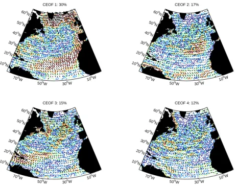
First, consider the results of the CEOF analysis for the whole North Atlantic basin. In Fig. 1 we plot the spatial patterns of the leading four CEOFs. Recall that the modes are complex-valued; we plot both the spatial CEOF amplitude (coloured contours) and

10

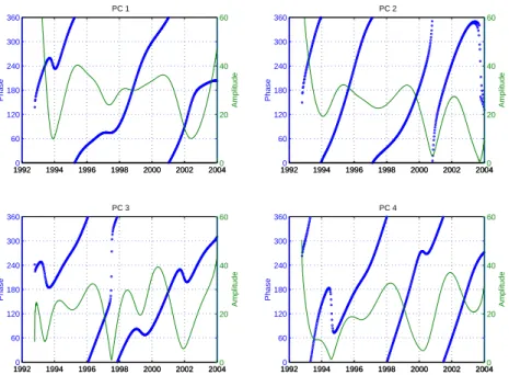
phase (arrows). In Fig. 2, we plot the complex-valued time series of the associated principal components: amplitude (green line) and phase (blue circles) time series are plotted for each. The leading CEOF mode represents 30% of the total SSH variability, and the sum of the first four modes accounts for 74%. We use the Lambert conical projection for the maps as it takes account of the latitudinal variation in length of a fixed

15

range of degrees in longitude.

It can be seen from Fig. 2 that the phase time series of PC1 (the principal component of the leading CEOF mode) has a dominant period of around 5 years. Looking at the corresponding amplitude map in Fig. 1, we note that there is a tripole-like structure: two domains of high SSH variability in the subpolar gyre and at low latitudes, with a

20

region of low variability between them. The two high variability regions at high and low latitudes are linked by a ridge of high variability along the eastern boundary. It is well known that there is a sea surface temperature tripole associated with the North Atlantic Oscillation (Marshall et al., 2001). However, although there appears to be a degree of similarity between the patterns in SST and the leading-mode SSH, the structures are

25

not the same.

There is some indication that the phase arrows in the leading-mode SSH along the eastern boundary rotate anticlockwise (a shift from pointing predominantly north off the African coast to northwest off the British Isles). This suggests that there is

(9)

propa-OSD

Full Screen / Esc

EGU

gating energy running northwards along the eastward boundary linking the subtropics and subpolar regions. There is also evidence of SSH propagation in the northwest At-lantic and Labrador Sea: a clear anticlockwise rotation of phase arrows as the location changes north from Newfoundland towards the west of Greenland.

The spatial pattern of the second CEOF (17% of the total variability) has a different

5

structure from the leading CEOF. The regions of high variability are concentrated in the eastern subtropical gyre between ∼30◦–40◦N and in the tropics (∼5◦–15◦N). The structure of SSH variability, with highs in the eastern basin, suggests a possible link with the East Atlantic Pattern. This is the second most prominent mode (after the NAO) of low-frequency atmospheric pressure variability over the North Atlantic (Barnston and

10

Livezey, 1987). We look at possible connections with climate indices in further detail in Sect. 3.3. As we see from Fig. 2, the phase time series of PC2 has a cycle of ∼3 years. We analyse the time-varying spectral energy of this time series by subjecting it to a wavelet analysis, the results of which are shown in Fig. 3 (in fact, the leading four PCs were subject to wavelet analysis to provide summary descriptions for Table 1,

15

but we only show the results for PC2 here). From top to bottom, we see: (a) the input time series (i.e. the phase of PC2); (b) the wavelet power spectrum of (a), where the dashed line indicates the cone of influence below which edge effects, arising from the finite length of the time series, become important (Torrence and Compo, 1998); (c) the global wavelet power spectrum, i.e. time integral of (b); (d) time series of the scale

20

average of (b) in the period range 2.5–3.5 years (to capture the dominant cycle of ∼3 years). In Table 1, we summarise the characteristics of all four leading modes for the 18-month lowpass filtered data in the North Atlantic Ocean.

3.2 Sea surface height variability in the Azores subtropical front 3.2.1 Interannual variability: lowpass filtering at 18 months

25

We now focus on the northeast Atlantic (20◦–40◦N, 50◦–10◦W), encompassing the Azores subtropical front. This region is rich in westward propagating Rossby waves

(10)

OSD

Full Screen / Esc

EGU

and eddies (Tokmakian and Challenor, 1993; Cipollini et al., 1997; Pingree 1997; Cipollini et al., 1998; Tychensky et al., 1998; Pingree 2002). Given the smaller geographical domain, we now have sufficient computing capacity to calculate CE-OFs for the DUACS dataset at its original high-resolution spatial gridding of (1/3)◦ longitude×(1/3)◦×cos(latitude). Figures 4 and 5, analogous to Figs. 1 and 2

respec-5

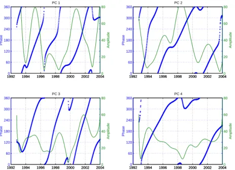
tively, show the results of the complex EOF analysis: amplitude and phase maps of the leading four CEOFs and the associated principal components. These four modes account for 79% of the total variability.

As shown in Fig. 4, the leading mode (35% of the total variability) is strong in the south and east, consistent with the NAO-related pattern found in Sect. 3.1 (North

10

Atlantic basin). Variability strength is around one order of magnitude lower north of ∼30◦N, except for the northeast region and a few isolated patches in the northwest quadrant. The second mode (21% of the total variability) has a different spatial distri-bution: a near-zonal band of lower variance between ∼22◦–27◦N sandwiched between two regions of higher variance. This reveals further details of the EAP-related structure

15

found earlier. Again, the levels of variance span around one order of magnitude. Mode 3 has a strong ridge of variability near 28◦N.

We performed wavelet analysis of the phase time series of all four leading princi-pal components to investigate time-dependent spectral energy changes. Fig. 6 shows the results for the phase of the leading mode which displays strong propagation at

20

∼3 years and ∼5 years (though the latter must be treated with caution in this smaller geographical domain because it falls beneath the cone of influence). In Sect. 3.1 above we noted that the EAP-related mode (second leading mode) had a dominant timescale of ∼3 years. The discovery of a ∼3 year component in the leading mode of SSH vari-ability in the subtropical Azores Frontal region suggests that the EAP may be playing a

25

strong role here. The scale-averaged energy in the period range 2–4 years (to capture the ∼3 year signal) decays gradually from a peak in 1994. The characteristics of all four leading modes for the 18-month lowpass filtered data in the region of the Azores subtropical front are summarised in Table 2.

(11)

OSD

Full Screen / Esc

EGU

3.2.2 Subannual baroclinic propagation: lowpass filtering at 30 days

As mentioned above, it is well known that westward propagating baroclinic Rossby waves can be seen in SSH observations in the mid-latitudes of the North Atlantic basin. In particular, a ‘waveband’ of enhanced SSH variability associated with such waves is concentrated in a quasi-zonal strip centred near 34◦N (Cromwell, 2001). The

5

period of these midlatitude waves are subannual (∼6–10 months); lowpass filtering at 18 months would therefore remove them. To study these signals, we therefore low-pass filter the data with a cutoff of 30 days, rather than 18 months, thus retaining the baroclinic Rossby wave signal but removing higher-frequency variability. We then per-formed CEOF analysis followed by wavelet analysis of the principal components, just

10

as before.

The leading mode is the annual steric signal which accounts for 46% of the total SSH variability. If this mode is discounted, the second mode has 10% of the remaining vari-ability and has three significant timescales at ∼3 years, ∼1 years and 6 months (not plotted). The third mode (6% of non-steric variability) displays properties consistent

15

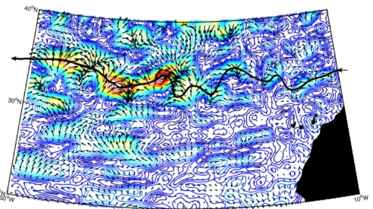
with propagating baroclinic Rossby waves. Figure 7 shows the spatial pattern of this mode, including the westward direction of propagation. Note the concentration of SSH variability in a near zonal band at 32◦–36◦N. Note, too, the anticlockwise rotation of the phase vector from east to west, consistent with westward propagation in this region. We have thus found for the first time, as far as we are aware, the variation in the

trajec-20

tory (in both longitude and latitude) of the propagation of Rossby waves in this region. By estimating the period (∼230 days) of this mode from the associated principal com-ponent (not plotted here), and the spatial distance over which a 360◦ rotation of the phase arrow occurs, i.e. the wavelength (∼520 km), we can estimate the speed of the Rossby waves at this latitude as ∼2.7 cm/s. This confirms earlier estimates (Chelton

25

and Schlax, 1996, Cipollini et al., 1997). CEOF mode 4 displays similar characteris-tics as mode 3, including the westward propagation. This indicates that the baroclinic Rossby wave energy is partitioned into both these modes, representing a total

(12)

variabil-OSD

Full Screen / Esc

EGU

ity of 11% of the non-steric SSH signal.

We then perform a wavelet analysis of the phase component of PC3, yielding de-tailed information about the phase propagation corresponding to the Rossby waves (Fig. 8). Figure 8b shows strong spectral content at the subannual periods charac-teristic of such waves at midlatitudes. There is also strong variability at periods of

5

2–4 years, though after 2001 this energy lies below the cone of influence (dashed line) and must be treated with caution (edge effects). In Fig. 8d, scale averaging over the period range of 0.5–0.8 years (∼6–10 months) shows the time-varying strength of the Rossby wave signal. There are peaks in 1996, 1997, 1999 and again in 2003. These are likely related to peaks in forcing. Finally, the characteristics of all four leading

10

modes for the 30-day lowpass filtered data in the region of the Azores subtropical front are summarised in Table 3.

3.3 Relationship of the North Atlantic Oscillation (NAO) and East Atlantic Pattern (EAP) to Sea Surface Height Variability

Atmospheric pressure variations play a role in forcing sea surface height variability.

15

To investigate a possible physical relationship between modes of atmospheric variabil-ity and SSH variabilvariabil-ity we used the climate indices provided by the National Oceanic and Atmospheric Administration/National Weather Service Climate Prediction Center (CPC). The two leading atmospheric pressure modes in winter are the North Atlantic Oscillation (NAO) and East Atlantic Pattern (EAP). The CPC indices are available from

20

http://www.cpc.ncep.noaa.gov/and are derived from an analysis based on the work of

(Barnston and Livezey, 1987).

We consider interannual SSH variations in (a) the North Atlantic (i.e. the work of §3.1) and (b) the Azores Subtropical Front (§3.2.1 above). As a measure of the strength of a mode of SSH variability, we use the amplitude of the corresponding principal

com-25

ponent. For both case (a) and (b) we calculated the cross-correlation coefficient (r) between the climate index (NAO and EAP) and the strength of each of the two leading complex EOFs. Table 4 summarises the results. We see that the NAO is correlated

(13)

OSD

Full Screen / Esc

EGU

only very weakly, if at all, with the leading principal component amplitudes of SSH variability. Indeed, in the Azores Subtropical Region, there is a hint of a very weak anti-correlation between the NAO and the amplitude of PC2. This is not altogether surprising: we noted earlier that although the spatial pattern of the leading mode has a tripole structure it is different from the SST tripole associated with the NAO.

Tempo-5

ral variability of the NAO likely maps onto more than simply the leading mode of SSH variability.

In contrast, the EAP is correlated with the two leading modes of SSH variability, particularly with PC2 in the Azores Subtropical Front region, where r=0.22. The cross-correlations of the two leading modes of SSH variability with the EAP index exceed

10

the 95% confidence level. The small values of r indicate that, although this mode of atmospheric pressure variability plays a significant role in explaining these modes of SSH variance, it is not the dominating factor. Modelling studies, beyond the scope of this study, would be required to investigate the relative role of possible forcing mecha-nisms such as baroclinic instability, bursts in wind stress or seasonal variations in local

15

currents.

4 Discussion and conclusions

We have investigated the variability of sea surface height in the North Atlantic basin using a merged DUACS altimeter dataset spanning October 1992–January 2004. By applying complex empirical orthogonal function analysis we determined the spatial and

20

temporal structure of SSH variability, including evidence of propagating features, for the leading four modes. Using wavelet analysis we determined the time-varying spectral density content of the principal components. We began by investigating the interan-nual variability in the North Atlantic by lowpass filtering the SSH data at a cutoff of 18 months. The spatial pattern of the leading complex EOF, comprising 30% of the total

25

variability, showed a tripole structure with a connecting ridge between the high-latitude region and the subtropics along the eastern boundary. The regions of strong variability

(14)

OSD

Full Screen / Esc

EGU

in the subtropics and subpolar gyre are linked by a 5-year signal propagating north along the eastern boundary. Rotation of CEOF phase arrows also indicates SSH prop-agation at 5-year periodicity in the Labrador Sea. The second mode, with a strong 3-year phase signal, is concentrated in the eastern subtropical gyre and may be linked to the low-frequency East Atlantic Pattern of atmospheric pressure variability.

5

We also focussed on the Azores subtropical front region of the northeast Atlantic. The leading mode (35% of the total variability) is strong in the south and east of this region. A dominant 3-year signal suggests that the EAP may be playing an important role in forcing SSH variability in this dynamic region. The second mode (21%) has a near-zonal band of lower variance between ∼22◦–27◦N sandwiched between two

10

regions of higher variance.

In order to retain SSH signatures associated with propagating baroclinic Rossby waves we also lowpass filtered the altimeter data in the northeast Atlantic at a 30-day (rather than 18-month) cutoff. The strongest mode is the annual steric signal, representing 46% of the SSH variability. The second mode, with dominant timescales

15

at ∼3 years, ∼1 year and 6 months accounts for 10% of the remaining variability. The third and fourth CEOFs, together accounting for 11% of the non-steric variability, are associated with westward propagating subannual Rossby waves which are particularly marked in a “waveband” between ∼32◦–36◦N. We showed the detailed trajectory of the westward propagating energy in this waveband. Peaks in the strength of this signal

20

are observed in the region in 1996, 1997, 1999 and 2003, presumably linked to strong forcing then.

No significant cross-correlation is found between the North Atlantic Oscillation and the amplitude of the leading two principal components of interannual SSH variability for either the North Atlantic basin or the subregion around the Azores subtropical front.

25

The East Atlantic Pattern, by contrast, is correlated with the principal components of the two leading modes of SSH variability, particularly with PC2 in the Azores subtropical frontal region.

(15)

OSD

Full Screen / Esc

EGU

sea surface temperature and chlorophyll to shed further light on the variability and dy-namics of the North Atlantic Ocean. Killworth et al. (2004), for example, have shown the potential for discriminating between different mechanisms involved in baroclinic Rossby wave propagation by combining sea surface height and chlorophyll observations from space. Further work on plausible forcing mechanisms on SSH variability could be

in-5

vestigated by comparing hindcasts for the observed time period of 1992–2004 from an ocean general circulation model with satellite and hydrographic measurements. Mod-elling studies, such as Eden and Willebrand (2001), have shown how hindcasts can shed light on mechanisms of interannual to decadal variability in North Atlantic SSH signatures and circulation. Bellucci and Richards (2006) also show the fruitfulness of

10

such an approach in their model investigation of the effect of decadal NAO variability on the ocean circulation in the North Atlantic. A combination of similar modelling and observational approaches will improve our ability to detect changes in the meridional overturning circulation which is of such importance to the climate system.

Acknowledgements. DUACS altimeter data were produced and kindly provided by the CLS

15

Space Oceanography Division. Paolo Cipollini helped make these data available to colleagues within the Laboratory for Satellite Oceanography at NOCS. Wavelet software was provided

by Christopher Torrence and Gilbert Compo, and is available at: http://paos.colorado.edu/

research/wavelets. The author gratefully acknowledges useful discussions with several col-leagues, especially P. Challenor, J. Harle, A. Hogg, J. Hirschi, S. Josey and B. Topliss. This 20

work was funded under the Ocean Variability and Climate core strategic programme of the UK’s Natural Environment Research Council.

References

Barnston, A. G. and R. E. Livezey: Classification, seasonality and persistence of low-frequency atmospheric circulation patterns, Mon. Weather Rev., 115, 1083–1126, 1987.

25

Bellucci, A. and Richards, K. J.: Effects of NAO variability on the North Atlantic Ocean circula-tion, Geophys. Res. Lett., 33, L02612, doi:10.1029/2005GL024890, 2006.

(16)

OSD

Full Screen / Esc

EGU Bryden, H. L., Longworth, H. R., and Cunningham, S. A.: Slowing of the Atlantic meridional

overturning circulation at 25◦N, Nature, 438, 655–657, 2005.

Chelton, D. B. and Schlax, M. G.: Global observations of oceanic Rossby waves, Science, 272, 234–238, 1996.

Cipollini, P., Cromwell, D., Jones, M. S., Quartly, G. D., and Challenor, P. G.: Concurrent al-5

timeter and infrared observations of Rossby wave propagation near 34◦N in the Northeast

Atlantic, Geophysical Research Letters, 24, 889–892, 1997.

Cipollini, P., Cromwell, D., and Quartly, G. D.: Observations of Rossby wave propagation in the northeast Atlantic with TOPEX/POSEIDON altimetry, Advances in Space Research 22, 1553–1556, 1998.

10

CLS: SSALTO/DUACS user handbook : (M)SLA and (M)ADT near-real time and delayed time products, Ramonville St-Agne-FRANCE CLS-DOS-NT-04.103, 2004.

Cromwell, D.: Sea surface height observations of the 34◦N “waveguide” in the North Atlantic,

Geophys. Res. Lett., 28, 3705–3708, 2001.

Eden, C. and Willebrand, J.: Mechanism of Interannual to Decadal Variability of the North 15

Atlantic Circulation, J. Clim., 14, 2266–2280, 2001.

Farge, M.: Wavelet transforms and their applications to turbulence, Annual Review of Fluid Mechanics, 24, 395–457, 1992.

Foufoula-Georgiou, E. and Kumar, P.: Wavelets in Geophysics, San Diego, Academic Press, 1994.

20

Fu, L.-L.: The interannual variability of the North Atlantic Ocean revealed by combined data from TOPEX/Poseidon and Jason altimetric measurements, Geophys Res. Lett., 31, L23303, doi:10.1029/2004GL021200, 2004.

Gill, A. E.: Atmosphere-Ocean Dynamics, San Diego, Academic Press, 662, 1982.

H ¨akkinen, S.: Variability in sea surface height: A qualitative measure for the meridional over-25

turning in the North Atlantic, J. Geophys. Res., 106, 13 837–13 848, 2001.

H ¨akkinen, S. and Rhines, P. B.: Decline of Subpolar North Atlantic Circulation During the 1990s, Science, 304, 555–559, 2004.

Jacobs, G. A., Hurlburt, H. E., Kindle, J. C., Metzger, E. J., Mitchell, J. L., Teague, W. J., and Wallcraft, A. J.: Decade-scale trans-Pacific propagation and warming effects of an El Ni˜no 30

anomaly, Nature, 370, 360–363, 1994.

Killworth, P. D., Cipollini, P., Uz, B. M., and Blundell, J. R.: Physical and biological mechanisms for planetary waves observed in sea-surface chlorophyll, J. Geophys. Res., 109, C07002,

(17)

OSD

Full Screen / Esc

EGU doi:10.1029/2003JC001768, 2004.

Le Traon, P. Y., and Ogor, F.: ERS-1/2 orbit improvement using TOPEX/Poseidon: the 2 cm challenge, J. Geophys. Res., 103, 8045–8057, 1998.

Le Traon, P. Y., Nadal, F., and Ducet, N.: An improved mapping method of multi-satellite altime-ter data, J. Atmos. Oceanic Technol., 25, 522–534, 1998.

5

Levermann, A., Griesel, A., Hofmann, M., Montoya, M., and Rahmstorf, S.: Dynamic sea level changes following changes in the thermohaline circulation, Clim. Dyn., 24, 347–354, 2005. Pingree, R. D.: The eastern Subtropical gyre (North Atlantic): Flow Rings Recirculations

Struc-ture and Subduction, J. Marine Biological Association of the United Kingdom, 77, 573–624, 1997.

10

Pingree, R. D.: Ocean structure and climate (Eastern North Atlantic): in situ measurement and remote sensing (altimeter), Journal of the Marine Biological Association of the UK, 82, 681–707, 2002.

Schiermeier, Q.: A sea change, Nature, 439, 256–260, 2006.

Tokmakian, R. T. and Challenor, P. G.: Observations in the Canary Basin and the Azores Frontal 15

Region Using Geosat Data, J. Geophys. Res. 98, 4761–4773, 1993.

Torrence, C. and Compo, G. P.: practical guide to wavelet analysis, Bulletin of the American Meteorological Society, 79, 61–78, 1998.

Tourre, Y. M., Kushnir, Y., and White, W. B.: Evolution of Interdecadal Variability in Sea Level Pressure, Sea Surface Temperature, and Upper Ocean Temperature over the Pacific Ocean, 20

Journal of Physical Oceanography, 29, 1528–1541, 1999.

Tychensky, A., Le Traon, P. Y., Hernandez, F., and Jourdan, D.: Large structures and temporal change in the Azores Front during the SEMAPHORE experiment, J. Geophys. Res., 103, 25 009–25 027, 1998.

von Storch, H. and Zwiers, F. W.: Statistical Analysis in Climate Research, Cambridge Univer-25

(18)

OSD

Full Screen / Esc

EGU Table 1. Summary of the characteristics of the leading four complex EOF modes of DUACS

altimeter sea surface height anomaly measurements in the North Atlantic basin (10◦–65◦N,

80◦–0◦W) for the period October 1992–January 2004. The input data are on a regular 1◦×1◦

grid, have a sampling period of 1 week and have been lowpass filtered to remove periods shorter than 18 months.

Mode % Variability Dominant timescales Notable features

1 30 ∼5 years Tripole structure; connecting ridge of

high variability at eastern boundary.

2 17 ∼3 years High variability in eastern subtropical

gyre and in western tropics. Amplitude low in 1997.

3 15 ∼2 years, ∼4 years High variability in western tropics,

Gulf Stream extension, Labrador Sea and in region of mid-Atlantic Ridge north of ∼35◦N.

4 12 > 3 years Isolated patches as well as ridges

of high variability, notably in western Labrador Sea. Amplitude peak in 2001.

(19)

OSD

Full Screen / Esc

altimeter sea surface height anomaly measurements in the northeast Atlantic (20◦–40◦N, 50◦–

10◦W) for the period October 1992–January 2004. The input data are on a high-resolution

Mercator grid of (1/3)◦ in longitude×(1/3)◦cos(latitude) in latitude, have a sampling period of 1

week and have been lowpass filtered to remove periods shorter than 18 months.

Mode % Variability Dominant timescales Notable features

1 35 ∼3 years, ∼5 years Strong variability south of 30◦N and also everywhere

east of ∼25◦W; one order of magnitude lower variability elsewhere.

2 21 ∼2 years, ∼5 years Near-zonal band of low variance at ∼22◦–27◦N

sandwiched between two regions of higher variance.

Again, the levels of variance span around one order of magnitude. Phase propagation with period of 2 years peaks in 2001.

3 13 ∼3 years Ridges and local patches of high

variability, including near-zonal band at 28◦N. Peak in phase propagation in 1997.

4 10 ∼4 years A few local patches of moderate

variability, mostly west of 35◦W. Strongest phase propagation between 1998–2001.

(20)

OSD

Full Screen / Esc

altimeter sea surface height anomaly measurements in the Azores Subtropical Front region

(20◦–40◦N, 50◦–10◦W) for the period October 1992–January 2004. The input data are on

a high-resolution Mercator grid of (1/3)◦ in longitude×(1/3)◦ cos(latitude) in latitude, have a

sampling period of 1 week and have been lowpass filtered to remove periods shorter than 30 days.

Mode % Variability Dominant

timescales

Notable features

1 46 Annual Steric cycle

2 5 ∼3 years

∼1 year ∼6 months

Peak in 1996

Observed between 2000–2002

Phase propagation observed 2001–2003

3 2.9 ∼6–10

months

Westward propagating baroclinic Rossby waves and/or eddies. concentration of SSH variability in a near zonal band

around 32◦–36◦N. Energy peaks occur in

winters of 1996, 1997, 1999 and 2003.

4 2.8 ∼6–10

months

(21)

OSD

Full Screen / Esc

EGU

Table 4. Cross-correlation coefficient (r) between climate indices NAO (North Atlantic

Oscilla-tion), EAP (East Atlantic Pattern) and the principal component amplitudes of the two leading

complex EOFs in the North Atlantic (10◦–65◦N, 80◦–0◦W) and Azores Subtropical Front (20◦–

40◦N, 50◦–10◦W) regions. Values of r inbold are statistically significant at the 95% confidence level.

NAO EAP

North Atlantic PC1_PC2 0.009_0.012 0.19_0.17

(22)

OSD

Full Screen / Esc

Printer-friendly Version Interactive Discussion EGU CEOF 1: 30% 70o W 50o_W 30oW 10 o_W 10o N 20o N 30o N 40o N 50o N 60o N CEOF 2: 17% 70o W 50o_W 30oW 10 o_W 10o N 20o N 30o N 40o N 50o N 60o N CEOF 3: 15% 70o W 50o_W 30oW 10 o_W 10o_N 20o N 30o_N 40o N 50o_N 60o_N CEOF 4: 12% 70o W 50o_W 30oW 10 o_W 10o_N 20o N 30o_N 40o N 50o_N 60o_N Figure 1

Fig. 1. Results of a complex empirical orthogonal function (CEOF) analysis of DUACS altimeter

sea surface height anomaly measurements in the North Atlantic basin (10◦–65◦N, 80◦–0◦W)

for the period October 1992–January 2004. The input data are on a regular 1◦×1◦grid, have

a sampling period of 1 week and have been lowpass filtered to remove periods shorter than 18 months. Maps of first four CEOF modes with amplitude contours (in arbitrary units) and phase overlaid as arrows (anticlockwise rotation of phase arrows from one location of strong amplitude to another indicates propagating signal). The title of each subplot gives the mode number and its percentage contribution to the total variability.

(23)

OSD

Full Screen / Esc

Printer-friendly Version Interactive Discussion EGU 19920 1994 1996 1998 2000 2002 2004 60 120 180 240 300 360 Phase PC 1 1992 1994 1996 1998 2000 2002 20040 20 40 60 Amplitude 19920 1994 1996 1998 2000 2002 2004 60 120 180 240 300 360 Phase PC 2 1992 1994 1996 1998 2000 2002 20040 20 40 60 Amplitude 19920 1994 1996 1998 2000 2002 2004 60 120 180 240 300 360 Phase PC 3 1992 1994 1996 1998 2000 2002 20040 20 40 60 Amplitude 19920 1994 1996 1998 2000 2002 2004 60 120 180 240 300 360 Phase PC 4 1992 1994 1996 1998 2000 2002 20040 20 40 60 Amplitude Figure 2

Fig. 2. Principal component time series corresponding to the maps of CEOF modes plotted

in Fig. 1 (North Atlantic SSH anomalies, 1◦×1◦ gridding, lowpass filtered at 18 months). Both

(24)

OSD

Full Screen / Esc

Printer-friendly Version Interactive Discussion EGU 1994 1996 1998 2000 2002 2004 0 2 4 6 8 Time (year)

Data (arb units)

a) Input time series

Time (year)

Period (years)

b) Wavelet Power Spectrum

1994 1996 1998 2000 2002 2004 0.25 0.5 1 2 4 8 0.25 0.5 1 2 4 8 0 50 100 150 200 250 Period (years)

Wavelet Power (arb units)

c) Global Wavelet Power Spectrum

1994 1996 1998 2000 2002 2004 0 0.5 1 1.5 Time (year) Avg variance

d) 2.5−−3.5yr Scale−average Time Series

Figure 3

Fig. 3. Wavelet analysis of the principal component phase associated with the second CEOF

in sea surface height anomaly in the North Atlantic (PC2 in Fig. 2). (a) Input time series,

i.e. the phase of PC2;(b) wavelet power spectrum of (a); (c) global wavelet power spectrum,

i.e. integral of (b) over time; (d) time series of scale average of (b) in period range 2.5–3.5

years. In (b), the dashed line indicates the cone of influence, below which edge effects become important, and the solid contour is the 95% confidence level. In (c) and (d), the 95% confidence level is indicated by a dashed line.

(25)

OSD

Full Screen / Esc

Printer-friendly Version Interactive Discussion EGU CEOF 1: 35% 50o_W 30oW 10 o_W 20o_N 30o N 40o N CEOF 2: 21% 50o_W 30oW 10 o_W 20o_N 30o N 40o N CEOF 3: 13% 50o_W 30oW 10 o_W 20o_N 30o N 40o_N CEOF 4: 10% 50o_W 30oW 10 o_W 20o_N 30o N 40o_N Figure 4

Fig. 4. Results of a complex empirical orthogonal function (CEOF) analysis of DUACS altimeter

sea surface height anomaly measurements in the northeast Atlantic basin (20◦–40◦N, 50◦–

10◦W) for the period October 1992–January 2004. The input data are on a Mercator (1/3)◦

longitude×(1/3)◦ cos(latitude) latitude grid, have a sampling period of 1 week and have been

lowpass filtered to remove periods shorter than 18 months. Maps of first four CEOF modes with amplitude contours (in arbitrary units) and phase overlaid as arrows (anticlockwise rotation of phase arrows from one location of strong amplitude to another indicates propagating signal). The title of each subplot gives the mode number and its percentage contribution to the total variability.

(26)

OSD

Full Screen / Esc

Printer-friendly Version Interactive Discussion EGU 19920 1994 1996 1998 2000 2002 2004 60 120 180 240 300 360 Phase PC 1 1992 1994 1996 1998 2000 2002 20040 20 40 60 80 Amplitude 19920 1994 1996 1998 2000 2002 2004 60 120 180 240 300 360 Phase PC 2 1992 1994 1996 1998 2000 2002 20040 20 40 60 80 Amplitude 19920 1994 1996 1998 2000 2002 2004 60 120 180 240 300 360 Phase PC 3 1992 1994 1996 1998 2000 2002 20040 20 40 60 80 Amplitude 19920 1994 1996 1998 2000 2002 2004 60 120 180 240 300 360 Phase PC 4 1992 1994 1996 1998 2000 2002 20040 20 40 60 80 Amplitude Figure 5

Fig. 5. Principal component time series corresponding to the maps of CEOF modes plotted in Fig. 4 (northeast Atlantic SSH anomalies, (1/3)◦×(1/3)◦cos(latitude) grid, lowpass filtered at 18 months). Both phase (in degrees; blue) and amplitude (arbitrary units; green) are shown.

(27)

OSD

Full Screen / Esc

Data (arb units)

Time (year)

Period (years)

1994 1996 1998 2000 2002 2004 0.25 0.5 1 2 4 8 0.25 0.5 1 2 4 8 0 50 100 150 200 Period (years)

1994 1996 1998 2000 2002 2004 0 0.2 0.4 0.6 0.8 1 Time (year) Avg variance

d) 2−−4yr Scale−average Time Series

Figure 6

Fig. 6. Wavelet analysis of the principal component phase associated with the leading CEOF in sea surface height anomaly over the northeast Atlantic (PC1 of Fig. 5). The dataset has been

lowpass filtered to remove signals shorter than 18 months.(a) Input time series, i.e. the phase

of PC1;(b) wavelet power spectrum of (a); (c) global wavelet power spectrum, i.e. integral of

(b) over time; (d) time series of scale average of (b) for periods in range 2–4 years. In (b),

the dashed line indicates the cone of influence, below which edge effects become important,

and the solid contour is the 95% confidence level. In (c) and (d), the 95% confidence level is indicated by a dashed line.

(28)

OSD

Full Screen / Esc

Printer-friendly Version Interactive Discussion EGU 50o_W 30o_W 10oW 20o_N 30o_N 40o_N Figure 7

Fig. 7. Spatial pattern of 3rd CEOF of sea surface height anomaly in northeast Atlantic after lowpass filtering at 30 days. Both amplitude (coloured contours; arbitrary units) and phase

(ar-rows) are shown. Phase rotation in the zonal band ∼32◦–36◦N west of ∼30◦W is characteristic

of the westward propagation of baroclinic Rossby waves in this region. The solid black line indicates the observed trajectory of the Rossby waves.

(29)

OSD

Full Screen / Esc

Data (arb units)

Time (year)

Period (years)

1994 1996 1998 2000 2002 2004 0.25 0.5 1 2 4 8 0.25 0.5 1 2 4 8 0 10 20 30 40 50 Period (years)

1994 1996 1998 2000 2002 2004 0 0.5 1 1.5 2 Time (year) Avg variance

d) 0.5−−0.8yr Scale−average Time Series

Figure 8

Fig. 8. Wavelet analysis of the principal component phase associated with the 3rd CEOF in sea surface height over the northeast Atlantic. The dataset has been lowpass filtered to

remove signals shorter than 30 days, thus retaining subannual variability.(a) Input time series,

i.e. the phase of the 3rd principal component; (b) wavelet power spectrum of (a); (c) global

wavelet power spectrum, i.e. integral of (b) over time;(d) time series of scale average of (b) for

periods in range 0.5–0.8 years (∼6–10 months), corresponding to baroclinic Rossby waves at this latitude. In (b), the dashed line indicates the cone of influence, below which edge effects become important, and the solid contour is the 95% confidence level. In (c) and (d), the 95% confidence level is indicated by a dashed line.