HAL Id: hal-00297176
https://hal.archives-ouvertes.fr/hal-00297176
Submitted on 4 Apr 2006
HAL is a multi-disciplinary open access
archive for the deposit and dissemination of
sci-entific research documents, whether they are
pub-lished or not. The documents may come from
teaching and research institutions in France or
abroad, or from public or private research centers.
L’archive ouverte pluridisciplinaire HAL, est
destinée au dépôt et à la diffusion de documents
scientifiques de niveau recherche, publiés ou non,
émanant des établissements d’enseignement et de
recherche français ou étrangers, des laboratoires
publics ou privés.
conditions using high-resolution mesoscale and
Lagrangian particle models
J. L. Palau, G. Pérez-Landa, J. Melia, D. Segarra, M. M. Millán
To cite this version:
J. L. Palau, G. Pérez-Landa, J. Melia, D. Segarra, M. M. Millán. A study of dispersion in
com-plex terrain under winter conditions using high-resolution mesoscale and Lagrangian particle models.
Atmospheric Chemistry and Physics, European Geosciences Union, 2006, 6 (4), pp.1105-1134.
�hal-00297176�
www.atmos-chem-phys.net/6/1105/2006/ © Author(s) 2006. This work is licensed under a Creative Commons License.
Chemistry
and Physics
A study of dispersion in complex terrain under winter conditions
using high-resolution mesoscale and Lagrangian particle models
J. L. Palau1, G. P´erez-Landa1, J. Meli´a2, D. Segarra2, and M. M. Mill´an1
1Fundaci´on Centro de Estudios Ambientales del Mediterr´aneo (CEAM), Val`encia, Spain 2Departamento de Termodin`amica, Facultat de F´ısica, Val`encia, Spain
Received: 6 October 2005 – Published in Atmos. Chem. Phys. Discuss.: 22 November 2005 Revised: 7 February 2006 – Accepted: 7 February 2006 – Published: 4 April 2006
Abstract. A mesoscale model (MM5), a dispersive
Lan-grangian particle model (FLEXPART), and intensive mete-orological and COrrelation SPECtrometer (COSPEC) mea-surements from a field campaign are used to examine the ad-vection and turbulent diffusion patterns associated with in-teractions and forcings between topography, synoptic atmo-spheric flows and thermally-driven circulations. This study describes the atmospheric dispersion of emissions from a power plant with a 343-m tall chimney, situated on very com-plex terrain in the North-East of Spain, under winter condi-tions. During the field campaign, the plume was transported with low transversal dispersion and deformed essentially due to the effect of mechanical turbulence. The main surface im-pacts appeared at long distances from the emission source (more than 30 km). The results show that the coupled models (MM5 and FLEXPART) are able to predict the plume inte-gral advection from the power plant on very complex terrain. Integral advection and turbulent dispersion are derived from the dispersive Lagrangian model output for three consecu-tive days so that a direct quantitaconsecu-tive comparison has been made between the temporal evolution of the predicted three-dimensional dispersive conditions and the COSPEC mea-surements. Comparison between experimental and simulated transversal dispersion shows an index of agreement between 80% and 90%, within distance ranges from 6 to 33 km from the stack. Linked to the orographic features, the simulated plume impacts on the ground more than 30 km away from the stack, because of the lee waves simulated by MM5.
1 Introduction
Dispersion of pollutants emitted from tall chimneys has been widely studied since the beginning of the twentieth
cen-Correspondence to: J. L. Palau
tury. The transport of air pollutants (mainly tracers and SO2
plumes) in stratified layers over land was documented in the US in the mid-to-late 1960s (Singer and Smith, 1966). Some of the available results were consolidated in the reports by Slade (1968) and ASME (1973) and reviewed by Pooler and Niemeyer (1971). For industrial stacks, the formation of sta-ble plumes was considered a rare phenomenon resulting from the emission of hot effluents into a stable atmosphere (with shear, for a thin but wide, “fanning-type” plume, and without shear, for a thin and narrow, “ribbon-type” plume). The most significant aspects of this phenomenon were that the plumes became very thin, under essentially no vertical diffusion, and could be found at large distances from their sources after one-night’s travel (Brown et al., 1972). It was also realised that the observed behaviour of the plume reflected the properties of the atmospheric layers in which it had become embedded. These observations became more and more frequent in the early 1970s with the tracking of plumes from tall stacks. Pas-sive remote sensing COrrelation SPECtrometer (COSPEC) measurement campaigns documented their travel distances to hundreds of km from the source (Mill´an and Chung, 1977; Mill´an, 1978b; Carras and Williams, 1981). They also docu-mented that stratified plumes could form and/or persist dur-ing the day, whenever conditions were right (Uthe and Wil-son, 1979; Portelli et al., 1982; Hoff and Gallant, 1985; Mill´an, 1987).
Passive remote sensing lidar measurements (measuring both mean values and turbulent components) have also been extensively used since the beginning of the 1970s to study tropospheric flows and the atmospheric dispersion of plumes emitted from point and area sources within the planetary boundary layer, PBL (Luhar and Young, 2002; Fast and Darby, 2004). Nevertheless, to the author’s knowledge, avail-able databases using lidar remote sensing technology and in-cluding simultaneous measurements of fumigations on the ground, are associated with field campaigns lasting only few days, e.g., the Nanticoke Shoreline Diffusion Experiment
(Hoff et al., 1982); the Kwinana Coastal Fumigation Study (Sawford et al., 1998) and the Vertical Transport and Mixing Program, VTMX (Doran et al., 2002).
The availability of measurements aloft enables us to ver-ify the patterns of advection and turbulent diffusion which govern atmospheric pollutant dynamics in complex topogra-phy areas (as a previous step to the analysis of the cause-effect relation between the emission source and the ground-level concentration). In complex topography, availability of simultaneous measurements aloft and at ground level is a clear advantage because surface concentrations and plume pathways aloft are not necessarily correlated (essentially due to the vertical wind directional shear and to the hetero-geneity of the physiographic thermodynamic properties of the ground). Moreover, ground-level pollutant concentra-tions typically present high spatial variabilities that are dif-ficult to simulate because they result from non-stationary three-dimensional circulations and recirculations of pollu-tants driven by valleys, hills, mountains and any other to-pographic feature (Zaremba and Carroll, 1999).
At present, most simulated dispersion results are gener-ally checked either against measurements of tracer-pollutant surface concentrations, with the dispersion analysis limited to the impact areas (Souto et al., 2001; Mart´ın et al., 2001; Fast, 1995; Fast et al., 1995; Luhar, 2002); or occasion-ally, against instrumented airplane measurements taken dur-ing field campaigns lastdur-ing several days (Carroll and Baskett, 1979; Mill´an et al., 1992). In this latter case, the measure-ments recorded along the airplane pathway are difficult to compare with simulated concentrations due to the former’s high temporal and spatial resolution1(Eastman et al., 1995; Carvalho et al., 2002).
Complementing the previously published studies per-formed in the Iberian Peninsula with correlation spectrome-ter techniques (as e.g., Albizuri, 1985; Mill´an et al., 1987, 1991; Alonso et al., 1987, 1993; Salvador et al., 1999; Arti˜nano et al., 1993; Querol et al., 1999; Palau et al., 2001), this paper presents what is to our knowledge the first dis-persive study using measurements aloft and on the ground simultaneously, together with numerical models resolving mesoscale forcings in the study area to reproduce the three-dimensional wind and turbulent fields.
In this study, the mesoscale model MM5, the dispersive Langrangian particle model FLEXPART, and the intensive meteorological and COSPEC measurements obtained during one of the “Els Ports-Maestrat” field campaigns are used to examine the advection and turbulent diffusion patterns un-der typical winter conditions that are associated with inter-actions and forcings between topography, synoptic atmo-spheric flows and thermally-driven circulations on a mid-latitude complex terrain. A unique aspect of this study is
1Simulated concentrations are generally hourly averaged (in
time and space), while measurements taken with an airplane are quasi-instantaneously recorded along the plane pathway.
that integral advection and turbulent dispersion are derived from the dispersive Lagrangian model output for three con-secutive days so that a direct quantitative comparison can be made between the temporal evolution of the predicted three-dimensional dispersive conditions and the COSPEC mea-surements. Nearly all of the COSPEC measurements are em-ployed. After the predicted dispersive conditions have been evaluated (analysing the integral advection of the plume aloft and the horizontal turbulent diffusion), we present the analy-sis of the ground impacts due to both meso and locally-driven flows, including the consequences of orographical effects on the simulated wind fields.
2 “Els Ports-Maestrat” field campaigns: Els Ports database
The Els Ports-Maestrat field campaign, sponsored by the En-vironment Department of the Valencia (Spain) regional gov-ernment, has been conducted at the Southwestern border of the Ebro basin since November 1994. One of the main ob-jectives of this field campaign is to monitor (aloft and on the ground) the SO2 plume emitted from the 343-m tall stack
of the Andorra Power Plant (APP) located at Teruel (Spain), Figs. 1 and 2. Another objective is to study the possible ef-fects on the APP emissions on the Els Ports/Maestrat forest masses. Thus, the “Els Ports” database consists, on the one hand, of three independent (but related) meteorological and air quality databases that extend from the end of 1994 to the present (2005), and, on the other hand, of a fourth database, complementary but independent from the plume monitoring, generated from a parallel monitoring of the state of the veg-etation in a network of selected plots within the study area.
The first database is constituted by a systematic tracking of the SO2-plume emitted from the APP (Teruel, Spain).
Measurements are performed at different distances from the chimney (along the available road network, Figs. 2 and 1b) with the double aim of (1) monitoring the plume’s atmospheric dispersion (advection+turbulent diffusion) and ground impacts over complex terrain under different meteo-rological conditions and (2) identifying (and quantifying) the recurrence of each dispersive scenario in this mid-latitude re-gion. The set of plume field measurements is very extensive; at present, it includes more than 3236 experimental plume-distributions registered spatially during the 1994–2004 pe-riod (equally distributed during the four annual seasons).
The second and the third databases are sets of measure-ments obtained from the Regional Air Quality Network (measuring continuously air pollutants and meteorological parameters), and from ENDESA (the power generation com-pany, owner of this power plant). The available meteorologi-cal data (wind direction, wind speed, temperature and short-wave radiation) are recorded electronically every 15 min at 10 m above the ground. Sensors are located on different sites in the area (Fig. 2), and they have different temporal coverage
Fig. 1. Modelling configuration with the five grids of different resolution employed in the simulations centred over the Andorra power plant
(G1108 km, G236 km, G312 km, G44 km; G51.3 km). Road network used by the mobile units (instrumented with a COSPEC) to take
measurements around the power plant is also indicated in white in the fifth grid.
because they were installed at different times during the last decade. Besides, ENDESA has two more meteorological towers located near the power plant; one is 60 m in height and the other (Monagrega) is 10 km away.
The fourth database consists of two types of forested plots: plots with conifers and plots where lichen transplants were made. This last database is not used further in the study presented in this paper, although it played an important role when defining the field campaigns (Palau, 2003).
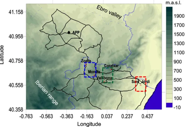
Fig. 2. Study area around the Andorra Power Plant (APP) in the North-East of the Iberian Peninsula, near the Mediterranean sea (bottom right
corner). Blue lines indicate borders of three Spanish provinces. Black lines indicate the available road network around the APP. Locations of five air quality and meteorological stations are also indicated; an additional 60 m-high meteorological tower is located beside the APP. Rectangles indicate the three different orographic areas where plume impacts on the ground were analysed by comparing the simulated results with measurements (area 1: blue color dashed square, area 2: green square and area 3: red square).
3 Study area
The Andorra Power Plant (APP) – ENDESA, 1050 MW – with a 343-m-tall chimney, is located near the city of An-dorra (Teruel), (00◦2204600W; 40◦5905400N), 87 km from the Spanish Mediterranean coast, in the Southwestern border of the Ebro basin (605 m above sea level (m a.s.l.). The APP, licensed for construction in 1974, would nowadays be considered a medium-size installation, with three genera-tors of 350 MW each. Nevertheless, it uses large amounts of low-grade lignite with high sulphur content (from 12 000 to 15 000 tons/day, with 5–6% sulphur content) (ENDESA, 1994), which translates into high SO2emissions (11.2 g/Nm3
in 1987).
The study area comprises three main basins (Fig. 2): the Mediterranean coast (East from the Power Plant), the Ebro valley (North from the Power Plant, running from NNW to ESE) and the Northeastern ridges of the Iberian Range (South and Southeast from the Power Plant).
The area includes the semi-arid plane of Calanda (100 km inland from the coast, with a mean altitude of 600 m a.s.l.), some mountain ranges on the Northwestern side of the Iberian Range (Mediterranean forest with a mean altitude of 1000 to 1300 m a.s.l) and the coastal plain of Castellon
(veg-etation characterised by irrigated crops). This coastal plain is delimited to the North, 7 km from the coast, by a moun-tain range of 780 m a.s.l. (with a very steep slope towards the coastal side).
Within this area, strong and extensive micro and mesoscale circulations develop, which are enhanced and driven by to-pography (Mill´an, 2002). Previous studies (Carroll and Bas-kett, 1979; Mill´an et al., 1992; Liu and Carroll, 1996; COST-710, 1998; Kitada et al., 1998; Zaremba and Carroll, 1999) have emphasized how complex terrain drives micro-and-meso-scale secondary circulations. These, superimposed on the general flow (synoptic scale), drive the advection of mo-mentum, energy, moisture and mass, within scales essentially different from those of turbulence (lower scale), which are the focus of “traditional” dispersion models. Secondary cir-culations are responsible for cumulus development (convec-tive clouds) associated with mountain barriers (Huggins et al., 2005), leewaves perturbing general flow streamlines of the lower troposphere, etc. In this sense, some studies under Foehn conditions have already been performed on the North coast of the Iberian Peninsula (Gangoiti et al., 2002) using RAMS2model.
2RAMS: Regional Atmospheric Modeling System: http://www.
Dispersive patterns characteristic of the elevated plume emitted from the 343 m-tall chimney are frequently the result of the interaction between these kinds of thermal and/or me-chanical circulations and flows driven by larger spatial scales (synoptic scale), Palau (2003).
In wintertime (from October to March), previous results (Palau, 2003) showed that the synoptic conditions driving Northwest advections represent up to 57% of the field cam-paigns carried out during the 1995–2000 winter period (study performed from a total of 112 different campaign days dur-ing that period). This dispersive scenario is associated, from a synoptic point of view, with anticyclonic conditions over the Iberian Peninsula and Southeastern Europe; it is one of the two most representative dispersive conditions prevailing in the Northeast region of the Iberian Peninsula (mainly as-sociated with neutral to stable atmospheric conditions). Un-der such winter meteorological conditions, with completely clear skies, temperatures around 0◦C and moderate-to-strong
Northwestern wind flows, the plume aloft is advected with very low transversal and vertical dispersion (ribbon-type in-tegral advective conditions) and it is deformed (differential advection) only by mechanical turbulence leeward mountain ranges (Palau et al., 2004). Thus, the main plume impacts on the ground are located far away from the chimney (more than 30 km), and generally within spatial areas on the ground that are in good agreement with the direction of the general wind flow aloft. Nevertheless, on occasion, intense fumiga-tions near the chimney, i.e. within 30 km, have been recorded in coincidence with either high wind-speed events (mechical turbulence) or low wind speeds around noon under an-ticyclonic conditions (convective turbulence associated with insolation and dry surface conditions).
4 Methodology
4.1 Experimental setup
To monitor the plume transport and ground-level fumigation we took systematic remote-sensing measurements using a mobile unit equipped with a Correlation Spectrometer Sys-tem – COSPEC – and a conventional SO2UV analyser, since
this equipment makes it possible to record the distribution of the pollutant both aloft and on the ground (Newcomb and Mill´an, 1970).
The COSPEC is a passive remote sensor that uses the sun-light dispersed in the atmosphere as its radiation source. Its response is proportional to the integral of the SO2
concen-tration (throughout the optic path between infinity and the instrument telescope). The pulsed fluorescence analyser is used to measure the SO2concentration over the roof of the
vehicle.
The plume-tracking strategy consisted of making tran-sects, as transversal as possible to the mean plume-transport direction, at different distances from the stack.
Measure-ments were taken throughout the day to record any changes that might occur in the plume transport direction or in the dispersive conditions (Fig. A1).
To obtain the dispersive parameters implicitly contained in the experimental data, Pseudo-Lagrangian averages were carried out (Mill´an, 1978b). This average is made with the coordinates related to the centre of gravity of each profile; thus, meandering effects are not taken into account. This profile, averaged in time but not in space, shows the relative diffusion of the plume and keeps its morphologic features (Mill´an et al., 1976): bifurcation, directional shear effect, wind-speed shear effect (i.e., Kurtosis), etc. Further details in Appendix A.
Concerning the available ground-based meteorological and air quality information, data from five air quality stations and from one 60 m-tall tower were available. The geograph-ical description for each site is as follows (Fig. 2):
The Morella station is located at the top of a 1160 m-high mountain, 50 km southeast of the Andorra power plant and 55 km inland from the Mediterranean coast. The Zorita sta-tion is located around 40 km from the power plant and at the bottom of a deep valley (the Bergantes valley). The Coratxar station is located 55 km southeast of the power plant and 42 km inland from the sea, at the top of a 1100 m-high mountain. The Vallibona station, 60 km from the chimney, is located SE from the power plant at 666 m a.s.l. The Sant Jordi station is located on a coastal plain North of the city of Castellon, about 80 km from the power plant and about 20 km from the Mediterranean coast. The 60 m-high meteorological tower, located at the power plant and near the chimney, mea-sures wind speed and direction at 60 m above ground level (m a.g.l.) and temperature at 10 m a.g.l.
Although the geographical distribution of the air quaility stations is biased towards the Southeast of the power plant (Fig. 2), this feature is not relevant to the present study because of the steady Northwest wind advection registered throughout the campaign.
There is no meteorological information aloft within the study area; thus, the comparison between the simulated wind fields aloft and those occurring during the campaign days was performed using measurements of the plume aloft (ob-tained with the COSPEC) as a tracer of opportunity of the wind flow at the mean plume transport height.
Total emission data available are monthly averages of the emission flow. Moreover, from the 60 m-high tower, meteo-rological measurements were recorded at 10 and 60 m a.g.l. every 15 min.
4.2 Model configuration
We used a non-hydrostatic mesoscale meteorological model MM5, version 3.2 (Dudhia, 1993; Grell et al., 1995) coupled to a Lagrangian Particle Dispersion (LPD) Model FLEX-PART, version 3.1 (Stohl, 1999; Stohl et al., 2005).
4.2.1 MM5 mesoscale meteorological model configuration The MM5 model used a nested-grid configuration with 5 do-mains (100×100 grids spaced at 108, 36, 12, 4 and 1.3 km, respectively) centred over the power plant (Fig. 1). The in-ner four domains are two-way interactive and are nested into the coarser domain, that is, run in 1-way mode. Thirty-nine sigma levels were configured, fifteen of them defined within the first 1500 m above ground level (m a.g.l.).
The model predicts the three-dimensional wind compo-nents u, v and w, the temperature, the humidity, the pres-sure perturbation and the associated turbulence parameters, as surface fluxes of heat, humidity and momentum. Multi-layer Blackadar Planetary Boundary Layer (PBL) parame-terization is employed to represent turbulent fluxes of heat, moisture and momentum (Zhang and Anthes, 1982). Bound-ary and initial conditions of atmospheric fields are derived from NCEP reanalysis data, available every 6 h at 2.5◦ reso-lution (Kalnay et al., 1996). Four-dimensional data assimila-tion (Stauffer and Seaman, 1994) was applied to the coarser domain, nudging towards the gridded reanalysis fields. Kain-Fritsch (1993) cumulus parameterisation was active in the three external domains.
Terrain data and properties like albedo, roughness and available soil moisture vary horizontally accordingly to the USGS (U.S. Geological Survey) topography and land use database, with 3000resolution.
4.2.2 FLEXPART Lagrangian particle disperson (LPD) model configuration
The FLEXPART-v3.1 model (Stohl, 1999) was fed by the MM5 meteorological outputs, using a grid configuration with one domain, which coincided with MM5 grid 5 (i.e., 100×100 grids spaced at 1.3 km and centred over the power plant).
The FLEXPART-LPD model takes into account wind ve-locity variances and Langrangian autocorrelations. The spread of the pollutant is simulated by the Langevin equa-tion derived by Thomson for inhomogeneous and Gaussian turbulence under non-stationary conditions (McNider et al., 1988). Lagrangian time scale is considered a function of the turbulent and stability conditions within the PBL. Turbulence statistics are obtained by using the Hanna scheme with some modifications taken from Ryall and Maryon for convective conditions (Stohl and Seibert, 2001). The Gaussian turbu-lence assumption is not strictly valid under convective condi-tions when the vertical velocity distribution is skewed. How-ever, the differences between a Markov process that includes wind velocity covariances and one that neglects them are likely to be very small as Uliasz (1994) showed when eval-uating different LPD model simplifications over mesoscale and regional areas. The FLEXPART model incorporates a density correction term for Gaussian turbulence which takes
into account the density decrease with height within the PBL (Stohl and Thomson, 1999).
The autocorrelation coefficient is assumed to be an expo-nential function that depends on the Lagrangian time scale. The time step used to move particles in the Markov chain model has to be variable in inhomogeneous turbulence and depends on the Lagrangian time scale (Uliasz, 1994). Well-mixed profiles can be obtained as long as the timestep is small enough to resolve the small-scale turbulence in the vicinity of the boundaries (Hurley and Physick, 1991).
Independently of the Langevin equation implemented within LPD models, to simulate dispersion from punctual anthropogenic point sources it is necessary to consider the emission heights of the Lagrangian particles.
A priori, from the available emission factors there is a large uncertainty when estimating the plume rise; thus we checked the eventual effect of plume-rise on the results ob-tained from the FLEXPART model by performing three inde-pendent dispersion simulations on the basis of three different plume-rise schemes:
– Releasing Lagrangian particles at variable heights,
esti-mated each hour using Briggs’ plume-rise equations for hot plumes (Briggs, 1975).
– Releasing Lagrangian particles at a constant height of
700 m a.g.l. (constant plume-rise of 357 m a.g.l.)
– Releasing Lagrangian particles at a constant height of
450 m a.g.l. (constant plume-rise of 107 m a.g.l.) It is important to note that these last two constant values are based on visual estimations of the plume-rise behaviour dur-ing the three-day campaign; they are considered to be the maximum and minimum plume-rise values observed at dif-ferent times of day during those three days. When using the Briggs’ plume-rise equations, quantitative analysis of the evolution of the simulated PBL and the height of the first in-version aloft allows us to set limits to the plume rise.
In our simulations, we treated the buoyant plume of the Andorra power plant by releasing 2×10⁶particles at different effective stack heights. The particles were randomly released and linearly distributed within a 0.1×0.1×0.01 km volume over 95-h period (from the beginning of the four-day simula-tion to the end).
From these dispersion simulations we obtain a time series of the three-dimensional distribution of Lagrangian particles (each one representing a specific volumetric concentration of pollutant).
4.3 Model validation
A wide variety of intercomparison procedures between ex-perimental and simulated air-quality results have been found to be useful (Fox, 1981; Willmott, 1981; Weil et al., 1992; Seaman, 2000). These procedures, strongly determined by
the number of available experimental data (data with a signif-icant spatial-temporal resolution), generally focus on the in-tercomparison of deviations in maximum values, first-order statistical momentum, frequency distribution of concentra-tion values, etc. (Carvalho et al., 2002; Fast et al., 1995; Uliasz, 1994; CityDelta web-page).
In our particular case, on one hand, the available data from the air quality network in the region have a good tempo-ral resolution but a coarse spatial resolution. On the other hand, although with a much coarser temporal resolution, “Els Ports” database has also an extensive field campaigns cover-ing the whole study area with a very good spatial distribution. The availability of surface information from the Air Qual-ity Network, and both surface and systematic tracking of the power plant plume aloft, allows a detailed validation of the skills of the aforementioned models (MM5+FLEXPART) in the simulation of the pollutants behaviour. Thus, the ability of the coupled models to simulate the two main physical pro-cesses driving air pollutant dispersion3(advection and turbu-lent dispersion) can be evaluated.
4.3.1 Direct comparison between plume tracking and model results
Using the plume transport direction aloft as a tracer of oppor-tunity of the wind field at the mean plume transport height, it is possible to make a direct comparison between the sim-ulated dispersive conditions with the measurements of the plume aloft. Thus, two different but complementary phys-ical processes can be analysed: (a) the integral-transport of the plume aloft, and (b) the turbulent dispersion (differential transport and turbulent diffusion) of the plume aloft. Addi-tionally, simultaneous measurements of SO2concentration at
surface level during the plume tracking, allows the compari-son between measured and simulated plume impact areas on the ground.
4.3.2 Comparison of the simulated and measured transver-sal dispersion
Obtaining typical horizontal deviations of the plume distri-bution aloft from the available experimental records has al-ready been described in the literature (Mill´an et al., 1976; Mill´an, 1978b); nevertheless, details of the modified Pseudo-Lagrangian method used in this study can be found in Ap-pendix A. In this study, it is important to remark that, fol-lowing this procedure and from the experimental measure-ments of the SO2distribution aloft, mean values of
transver-sal plume dispersion are obtained at different distances from the emission point and during a determinate temporal period.
3Following the terminology by Moran (2000). Within this
pa-per, advection is considered the sum of integral transport and differ-ential transport. Turbulent dispersion is considered as differdiffer-ential transport plus turbulent diffusion.
Fig. 3. Schematical representation of the procedure for
estimat-ing simulated transversal dispersion for fixed time periods and dis-tances. It shows the process for reducing a three-dimensional distri-bution of Lagrangian particles, N (x, y, z) during a time interval 1t, to a bi-dimensional distribution, N (y, z), at a fixed distance from the point source, x±dx. Finally, the standard deviation of N (y, z) is calculated as the vertical integration of the bi-dimensional La-grangian distribution.
The procedure for estimating simulated transversal disper-sion for fixed time periods and distances, Fig. 3, consists of reducing the three-dimensional distribution of Lagrangian particles to a bi-dimensional distribution (adding all the par-ticles vertically) contained within a plane that is normal to the direction determined by the centre of gravity of the sim-ulated particles during the fixed temporal period (the “simu-lated effective plane”, Fig. A2). Moreover, the distance to the source completely determines that effective plane (that dis-tance is fixed by the disdis-tance between the experimental effec-tive plane and the chimney; further details in Appendix A).
4.3.3 Comparison of spatial biases between measured and simulated ground-level SO2concentrations
The spatial density of the Air Quality Network is not enough to perform a detailed evaluation of the simulated ground-impact areas. However, availability of continous SO2
-concentration measurements at the five sites, allowed the quantification of spatial biases between the measurements within the study area and the simulated ground-concentration field during the whole period considered. Thus, it is possible to evaluate the performance of the model simulating ground-level concentrations during the different turbulent regimes implemented in the meteorological model.
Fig. 4. Synoptic chart (grid 2) at 18:00 GMT on 28 November 2001. Typical anticyclonic conditions prevailed during the experimental
campaign. Cross-isobaric flows advected the plume aloft towards the SE of the power plant (red cross at the North-East of the Iberian Peninsula).
5 26–28 November case study
The campaign of 26–28 November was selected as repre-sentative of the most recurrent winter scenarios in the area (winter Northwest advection, Appendix B); Palau, 2003. The analysis of synoptic conditions using NCEP Reanalysis data (Kalnay et al., 1996) and the meteorological datasets avail-able in the region (not shown), confirm that typical winter conditions prevailed during the experimental campaign. On these days, meteorological situation within the study area was driven synoptically by three main pressure systems: an Atlantic anticyclone extending over the Iberian Peninsula, a Low located over the North of the British Isles and an-other low pressure system located on the Western Mediter-ranan Sea. This synoptic configuration (Fig. 4) drove cross-isobaric flows, advecting the plume aloft towards the SE of the power plant (almost parallel to the Ebro valley axis to-wards the Mediterranean Sea) and inhibiting the develop-ment of thermally-driven local circulations. The passing of a cold front between 26 and 27 November, diminished tem-peratures and brought heavy cloudiness over the study area. After the cold front, skies cleared and wind speed increased substantially.
Forty transects (or, as previously indicated in the “Experi-mental setup” section, simultaneous recordings of the spatial SO2distribution aloft and on the ground) were performed at
different distances from the stack during the three-day cam-paign. Measurements were taken during the day and are
con-sidered representative of the dispersive conditions around the APP during the field campaign.
The mesometeorological simulation was initialized on 25 November to avoid spin-up effects on the simulated results for the first day of the campaign and was run for four days. Meteorological simulated fields were used to drive the LPD model simulations during the same period.
6 Results and discussion
Time series of vertical profiles of wind field (Fig. 5a) and temperature (Fig. 5b) at the stack location during the whole simulated period, show the main meteorological features de-scribed previously. The passing of a cold front between 26 and 27 November, can be identified by the wind speed in-crease, a decrease in temperature (Fig. 5b) and the wind direction turning towards the South (Fig. 5a) between the days 26 and 27. The simulated time series for the wind field and potential temperature show the predicted meteoro-logical conditions for the three different emission schemes implemented in the LPD model (constant heights of 450 and 700 m, and variable heights following the modified Briggs’plume-rise equations for hot plumes – Briggs, 1975; as indicated by colour lines, Figs. 5a and b). With respect to the dynamic emission conditions (wind speed and direction) for each of the three emission schemes no major differences are detected between them (Figs. 5a and b).
Fig. 5. Time series of the vertical profiles of wind field (left, a) and potential temperature (right, b) at APP site showing the meteorological
conditions for the three different emission schemes implemented in the LPD model (constant heights of 450 and 700 m, and variable heights following Briggs’ modified plume-rise equations for hot plumes; as indicated by coloured lines in panel a).
On the power plant site, the simulated PBL has a height of 700-to-800 m a.g.l. on the 25th, 26th and 29th of Novem-ber (not shown). On the 27th, after the cold airmass inflow and the wind speed increase, PBL ranges between 900 and 1200 m a.g.l. Besides, during the four simulated days, the simulated PBL is characterised by a surface layer in a muf-fled mechanical turbulence regime during the nocturnal hours (second category of the Blackadar parameterization imple-mented within MM5) with a PBL in a non-local free convec-tion regime (fourth Blackadar category) only for two-to-five hours around noon (when incoming short-wave radiation is higher).
6.1 Plume tracking versus model results
As representative of the results obtained from the three emis-sion schemes implemented in the LPD-model simulations, in this section we only present figures from the simulation performing the constant 700 m-high emission scheme. Com-parison between the measured plume dynamical behaviour throughout the day and the simulation is presented at dif-ferent instants during the day, corresponding to the difdif-ferent dispersive conditions identified: (a) During the early morn-ing and afternoon, measurements correspond to the nocturnal drainage flow where synoptic flows drive the plume dynam-ics and local mechanical turbulence governs the differential advection and diffusion (stirring and mixing) of the plume aloft but without major ground fumigations on the plane ar-eas near the chimney; (b) during the rest of the day, until the afternoon, thermal mesoscale circulations (convection) affect the plume dynamics favoring plume fumigations near the chimney.
6.1.1 Day: 26 November 2001
For the first campaign day (the second simulated day), two instants are shown (Figs. 6a and b) as representative of the dispersive conditions throughout the day. The first corre-sponds to midday and the second to five hours later (late af-ternoon).
Experimental measurements show the plume aloft being advected eastward from the power plant during the whole day. This is mostly captured by the simulation, although a small deviation towards the South can be observed in the late afternoon (Figs. 6c and d). At noon, SO2-ground level
con-centrations were measured South of the mean plume trans-port direction aloft (along a mountainous barrier, 45 km from the chimney). Thus, from the integral-transport point of view, on this first campaign day, westerly winds prevailed according to both the simulation (Figs. 6c and d) and the measurements (Figs. 6a and b) of the the plume aloft.
The main simulated SO2 ground-level concentrations are
spatially well correlated with the mean plume transport direc-tion aloft (Figs. 6a, b, c, d, e and f). The highest SO2ground
impacts are located leeward of mountain barriers and at dis-tances from the power plant ranging between 30 and 50 km. The lowest SO2ground impacts are also simulated and
mea-sured at shorter distances from the chimney, coinciding with periods with high short-wave radiation (associated with the free convection scheme performed by the MM5).
6.1.2 Day: 27 November 2001
To present the dispersive conditions for this second cam-paign day, we have selected three different instants during the day: in the morning, at noon, and in the late afternoon (Figs. 7a, b and 8a). On this day, simulated and observed
Fig. 6. First campaign day (26 November 2001). Top (a, b): COSPEC measurements of both the plume aloft (blue line) and its simultaneous
impacts on the ground (red line); (a: 10:45–11:58 GMT; b: 16:01–16:16 GMT). Middle (c, d): Simulated Lagrangian distribution at 11:00 GMT (left) and 16:00 GMT (right). Bottom (e, f): Simulated SO2concentrations on the ground at 11:00 GMT (left) and 16:00 GMT
Fig. 7. Second campaign day (27 November 2001). Top (a, b): COSPEC measurements of both the plume aloft (blue line) and its
simulta-neous impacts on the ground (red line); (a: 08:35–09:27 GMT; b: 11:03–11:50 GMT). Middle (c, d): Simulated Lagrangian distribution at 10:00 GMT (left) and 11:00 GMT (right). Bottom (e, f): Simulated SO2concentrations on the ground at 10:00 GMT (left) and 11:00 GMT
Fig. 8. Second campaign day (27 November 2001). Top-left (a): COSPEC measurements (15:41–15:52 GMT) of both the plume aloft (blue
line) and its simultaneous impacts on the ground (red line). Top-right and bottom (b, c): Simulated Lagrangian distribution (bottom) and SO2concentrations on the ground (right) at 16:00 GMT.
plume aloft is advected southeastward from the power plant during the entire day. Thus, from the integral-transport point of view, after the cold front passed, both the simulation and the experimentally-measured plume transport direction aloft changed towards the Southeast. During the afternoon, as a consequence of the wind speed increase at the plume trans-port height, the plume became thinner. A slight decrease in the transversal dispersion was observed due to wind speed increase during the afternoon (Figs. 6, 7 and 8, Table 1). The direction of the simulated plume seems to be slightly biased towards the South at 11:00 GMT (Figs. 7b and d) and at 12:00 GMT (Figs. 8a and b).
The measured SO2 ground impacts were light at short
distances from the chimney in the morning, they increased around noon, and they began to decrease again during the af-ternoon. During this second campaign day, Figs. 7 and 8, the
simulations also follow the experimentally recorded plume impacts on the ground. On the one hand, the highest impacts are simulated leeward of the mountain barriers and, on the other hand, the impacts close to the chimney are mainly sim-ulated during the periods of time associated to the strongest convective activity. Changing the convective scheme used by the MM5 model within the PBL produces a reduction in the number of impacts on the ground near the chimney during the afternoon (compare Figs. 7f and 8c).
Under these dispersive conditions, the simulated plume “footprint” (ground-level SO2 concentration) gives a good
sense of the preferred plume advection aloft. 6.1.3 Day: 28 November 2001
As the previous day, throughout this third campaign day the plume aloft continued to advect southeastward from the
Table 1. Experimental and simulated horizontal turbulent diffusion. Simulated values correspond to the three different emission schemes
performed (constant heights: 450 and 700 m a.g.l., and Briggs’ plume-rise scheme).
Day/ Hour Hour Distance Experimental Simulated Simulated Simulated Month Begin. End. (km) Dispersion dispersion dispersion dispersion (km) Briggs (km) 700 m (km) 450 m (km) 26 Nov 10:45 11:58 26.68 3.03 1.70 1.33 3.18 26 Nov 13:21 14:12 20.57 1.14 1.64 1.40 1.29 26 Nov 15:12 15:35 15.79 2.49 1.59 1.05 1.75 26 Nov 16:01 16:16 12.33 1.02 0.55 0.90 2.01 27 July 08:35 09:45 8.04 0.94 0.40 0.25 0.34 27 July 09:45 10:25 13.02 1.69 1.22 0.50 1.03 27 July 11:03 13:15 32.78 2.45 2.19 1.63 2.14 27 July 14:23 15:04 6.87 0.58 0.76 0.84 0.73 27 July 15:06 15:40 14.99 1.05 1.74 1.85 1.90 27 July 15:41 16:09 6.40 0.86 0.50 0.69 0.81 28 Nov 08:17 09:54 19.84 1.00 0.83 0.56 0.74 28 Nov 09:55 11:00 6.18 0.85 0.00 0.00 0.50 28 Nov 11:01 11:56 7.41 1.54 0.84 0.50 0.73 28 Nov 11:57 13:09 6.33 1.13 1.01 0.93 0.84 28 Nov 14:16 14:44 6.31 0.93 0.50 0.49 0.87
power plant. Thus, from the integral-transport point of view, both the simulation and the experimentally-measured plume transport direction aloft remain towards the Southeast. Temporal evolution of the simulated integral transport aloft, (Figs. 9c, d; 10c, d and 11b), shows that the model present very good skills, capturing the observed plume horizontal meandering.
In the early morning of the third campaign day, Fig. 9a, there are no measured impacts over the areas closest to the chimney, and the simulation only shows impacts leeward of mountain barriers 40-to-50 km from the power plant (there are no available mobile unit measurements in these areas dur-ing this period).
As on the previous day, around noon (Figs. 9b, d, f and Figs. 10a, c, e), the convective activity causes strong im-pacts on the ground near the power plant (as the experimental measurements show, Figs. 9b and 10a) and these are well-simulated by the LPD model (Figs. 9f and 10e). Around 13:00 GMT, the impacts close to the chimney cease (exper-imentally documented, Fig. 10b); around the same time of day, the LPD model performed a progressive reduction of impacts near the point source (Fig. 10f).
During the afternoon (14:45 to 15:40 GMT), the mobil unit recorded a channelization of the plume along the Bergantes valley (southeast from the chimney), with SO2ground-level
concentrations along the whole valley. In agreement with these measurements, simulated SO2 impacts on the ground
are recorded along the whole Bergantes valley (Southeast from the chimney) as a result of a topographically channel-ized simulated plume (Figs. 11a and c). In addition, the sim-ulated strong SO2ground impacts leeward of the mountains
still remain.
6.2 Horizontal turbulent diffusion
Under the aforesaid dispersive scenario (synoptic Northwest winter advection) a good correlation between experimental and simulated transversal dispersion was obtained within a spatial area ranging between 6 and 33 km (Fig. 12 and Ta-ble 1).
Results show that the LPD model systematically underes-timates transversal dispersion. Independent of the emission scheme performed, fittings between experimental and sim-ulated transversal dispersion values have slopes lower than one (Fig. 12, Tables 1 and 2). Nevertheless, better results are obtained when using the Briggs’ plume-rise scheme and the constant 450 m-height scheme (both schemes have excellent statistical significance4for the slope). From the 26th, these two emission schemes (Briggs and 450 m-height) present al-most the same advective conditions all the time, which is not the case for the 700 m-height scheme (Fig. 5a). Larger differences between the estimated plume rise obtained from the Briggs’ scheme and the 450 m-height scheme occur when very little vertical windspeed shear is simulated. On the con-trary, when major vertical windspeed shear is simulated (with important differences between the 450 m and 700 m heights) Briggs’ plume-rise is estimated around the 450 m-height.
Mean square errors (MSE) obtained from the linear fittings are lower than one kilometre, of the order of the available measurement spatial resolution (Table 2). The adimensional index of agreement (IoA), Willmott (1981), is higher than
4General criteria is: p-value≤0.001 (***, excellent
signifi-cance); p-value≤0.01 (**, good signifisignifi-cance); p-value≤0.05 (*, sig-nificant); p-value>0.05 (•, no significance).
Table 2. Statistical skills for the horizontal dispersion values simulated with the three different emission schemes. m: fitting slope; b: ordinate
[km]; SE: Standard Error; MSE: Mean Squared Error; MSEu: Unsystematic Mean Squared Error; MSEs: Systematic Mean Squared Error; MSEa: Additive Mean Squared Error: MSEp: Proportional Mean Squared Error; MSEi: Interdependence Mean Squared Error; d: Index of Agreement. “Rs” indicate “Root” for every statistic.
m b[km] SE (m) SE (b) [km] p-value (m) p-value (b)
450 m 0.81 0.13 0.20 0.30 0.001 0.667
700 m 0.31 0.43 0.18 0.28 0.108 0.141
BRIGGS 0.60 0.20 0.17 0.26 0.003 0.468
RMSE [km] RMSEu RMSEs RMSEa RMSEp RMSEi
450 m 0.53 0.49 0.18 0.13 0.29 −0.26
700 m 0.84 0.45 0.71 0.43 1.07 −0.91
BRIGGS 0.62 0.43 0.44 0.20 0.61 −0.46
MSEu/MSE MSEs/MSE MSEa/MSE MSEp/MSE MSEi/MSE d
450 m 0.88 0.12 0.06 0.30 0.25 0.94
700 m 0.29 0.71 0.27 1.62 1.17 0.80
BRIGGS 0.48 0.52 0.10 0.98 0.56 0.90
90% for the simulations using the Briggs’ and 450 m-height schemes, while it is 80% for the simulation using a constant 700 m-height scheme.
A dependence is detected between the emission scheme performed and the contribution of systematic and un-systematic errors to the total MSE. Whereas with the 450 m-height scheme a systematic contribution of 12% to the total MSE was obtained, with the Briggs’ equations the systematic contribution was 52%.
The un-systematic contribution to the total MSE and its absolute value (of the order of the experimental uncertainty) are indicative of the viability of this kind of numerical ap-proximation for performing dispersive studies over this kind of mid-latitude complex orography and under these winter dispersive conditions.
The systematic errors obtained could be directly related to uncertainties when describing land use and PBL physics. In this sense, further studies should be performed to quantify the effect of using different PBL parameterisations to de-scribe turbulent fields (and, therefore, pollutant dispersion) over mid-latitude complex terrain.
6.3 Plume impacts on the ground
If we compare the three simulated SO2 concentrations
ac-cumulated throughout the three-day campaign, it is clear that under the aforesaid meteorological conditions there are no qualitative differences between the plume “footprints” when using the three different emission schemes performed (Figs. 13a, b and c). This result is a direct consequence of the very similar dynamic conditions of the simulated emissions (Figs. 5a and b). Obviously, mechanical effects associated with topography are stronger in the case of the 450 m-high
fixed emission scheme than in the other cases; even so, the spatial pattern of the accumulated simulated impacts does not essentially vary with respect to the other two emission schemes (Figs. 13a, b and c). In the next section, the sim-ulated mechanical processes associated with the simsim-ulated ground impacts leeward of mountains are discussed.
To quantify the ground impacts of the plume aloft on the complex terrain around the emission source, we estimated the accumulated values of the simulated SO2 ground-level
concentrations for the different turbulent regimens imple-mented within the MM5. For this reason, we disaggre-gated the accumulated concentrations in the different turbu-lent regimes identified during the whole campaign. In this specific case, calculations were done separately for diurnal hours (free convection regime) and for nocturnal hours (muf-fled mechanical turbulence regime).
During the nocturnal hours, the accumulated ground-level concentrations show a strong bias towards areas leeward of the mountains, with no simulated impacts near the power plant (Fig. 14c). As a result, the closest simulated impacts are located 45 km away from the chimney. These results are in agreement with the experimental data that confirm that rele-vant impacts are located leeward of the mountains (Fig. 14d). In contrast, during the daytime, although the strongest im-pacts are simulated leeward of the mountains, significant ac-cumulated impacts are simulated in a wider area and closer to the chimney than for the nocturnal hours (Fig. 14a). This is coherent with the behaviour of the measurements in the five sites available (Fig. 14b).
Considering the spatial distribution of the SO2
accumu-lated magnitudes measured and the location of the five air quality stations, we have grouped them into three differ-ent geographical areas with the objective of intercomparing
Fig. 9. Third campaign day (28 November 2001). Top (a, b): COSPEC measurements of both the plume aloft (blue line) and its simultaneous
impacts on the ground (red line); (a: 08:17–09:54 GMT; b: 11:20–11:38 GMT). Middle (c, d): Simulated Lagrangian distribution at 09:00 GMT (left) and 11:00 GMT (right). Bottom (e, f): Simulated SO2concentrations on the ground at 09:00 GMT (left) and 11:00 GMT
Fig. 10. Third campaign day (28 November 2001). Top (a, b): COSPEC measurements of the plume aloft (blue line) and its simultaneous
impacts on the ground (red line); (a: 12:15–12:25 GMT; b: 12:59–13:09 GMT). Middle (c, d): Simulated Lagrangian distribution at 12:00 GMT (left) and 13:00 GMT (right). Bottom (e, f): Simulated SO2concentrations on the ground at 12:00 GMT (left) and 13:00 GMT
Fig. 11. Third campaign day (28 November 2001). Top-left (a): COSPEC measurements (14:45–15:40 GMT) of both the plume aloft (blue
line) and its simultaneous impacts on the ground (red line). Top-right and bottom (b, c): Simulated Lagrangian distribution (bottom) and SO2concentrations on the ground (right) at 14:00 GMT.
the experimental accumulated concentrations with the LPD model results within the same spatial areas. Figure 2 shows the spatial coverage of the three selected areas (1, 2 and 3), where the corresponding sites recorded accumulated SO2
ground-level concentrations lower than 1000 µg/m3, higher than 3000 µg/m3 and about 2000 µg/m3, respectively. To quantify the differences and the similarities between the sim-ulated and measured impact patterns, diurnal/nocturnal per-centual variations of the SO2 ground-level concentrations
were calculated as spatial averages within each of the afore-said zones of the study area (Fig. 2 and Table 3).
From the comparison between the experimental results and the simulated SO2 ground-level concentration fields
obtained using the three different emission schemes, we found that zones one and three have comparable diur-nal/nocturnal percentual contribution to the total SO2
con-centrations within each zone (Table 3). Both the simulated and experimentally measured results show a diurnal predom-inance in zone one and a higher nocturnal contribution in zone three. It is interesting to note the high variability of the percental contributions in area 3, depending of the emission scheme employed. This could suggest high spatial and tem-poral wind field variability at the leeward of the mountains, as small differences in the dynamical conditions of the emis-sions from the APP induce high variations of the simulated ground-level SO2concentration.
The discrepancy between the simulated results and the ex-perimental measurements within zone two is due to the direct plume impact at Coratxar station on the night of the 26th. At this site, a very intense plume impact was recorded on the 26th during the nocturnal hours (maximum 1-h average value of 1638 µg/m3, not shown). These extremely high SO2
Table 3. “Day/night” percentual variation in the mean ground-level SO2concentrations throughout the field campaign at three different areas
Southeast from the APP. Positive variations indicate that diurnal impacts prevail; negative variations indicate that nocturnal impacts prevail. Values are expressed in % and are calculated from 100×[SO2]day-[SO2]night/[SO2]day. This table is related to Fig. 14.
Day/night percentual variation of SO2ground-level concentrations
Experimental Emission 450 m Emission 700 m Briggs emission Briggs
AREA 1 57.7 100.0 100.0 100.0
AREA 2 −113.1 90.6 85.4 80.9
AREA 3 −122.6 −295.8 −92.2 −796.4
Fig. 12. Comparison between simulated and measured horizontal
diffusion for the three different emission schemes performed during the dispersive simulations. Values plotted in this figure are listed in Table 1 (downwind distances between 6 and 33 km).
concentration values, together with the low wind speed mea-sured (not shown), indicate that this plume impact was not associated with mechanical turbulence but rather with a di-rect plume impact on this site. Under very stable conditions with a completely thermalised plume (55 km away from the chimney) and with no external forces except gravity, direct plume impacts can occur at mountain heights similar to the plume advective height because the plume cannot change its internal energy to rise up the edge of the mountain (i.e., no variation in the plume external parameters and/or heat trans-fer with the environment is possible under such thermody-namic states).
To analyse the discrepancy between the simulation and the measurements it is necessary to consider, on the one hand, that this kind of episode (given its local nature) cannot be considered representative of the whole zone two (within which the average SO2concentration was calculated for the
four simulated days). On the other hand, under such sta-ble dispersive conditions (plume advected as a ribbon-type plume) slight deviations between the real and the simulated plume advective direction have a strong impact when com-paring simulated and measured local ground-level concen-trations (and this limitation worsens even more on complex terrain). Additionally, the analysis of the simulated results in-dicated the PBL parameterization overestimated the mechan-ical turbulence, avoiding a stable regime and consequently the presence of very high SO2concentrations.
6.4 Orographic effects on the simulated wind fields Mesometeorological model behaviour is analysed with re-spect to wind field perturbations due to complex orography, which drive plume impacts on the ground far away (>30 km) from the power plant considered in this study. As there are no available vertical measurements over the leeward areas, it is not possible to make a direct comparison between the sim-ulated turbulent fields and those produced within the study area under winter Northwest advective conditions. Nev-ertheless, description of the simulated wind field is neces-sary to complement some of the aforesaid physical processes when describing the temporal evolution of SO2ground-level
concentrations on the mountainous and coastal sites located Southeast of the APP.
For stationary flows, the development of trapped leewaves (leeward of mountain barriers) is favoured when a vertical increase in wind speed exists, i.e., when stability decreases with height. Scorer (1997) showed how these requirements are equivalent to the vertical decrease with height of the Scorer parameter (l2): l2= g U2 1 θ ∂θ ∂z− 1 U ∂2U ∂z2 (1)
(a) (b)
(c)
Fig. 13. Simulated plume footprint when using the three different emission schemes (top left, (a), 450 height; top right, (b), 700
m-height; and bottom, (c), Briggs’ plume-rise scheme). Figures represent the SO2ground-level concentration accumulated during the four-day
simulated period (25–28 November).
where
Uis the mean wind speed, perpendicular to the obstacle (or mountain).
gis the gravity acceleration.
θis the potential temperature.
As evidenced previously, within the context of complex-terrain air quality simulations, the ground-level plume im-pacts simulated leeward of the mountains represent one of the most relevant features of the dispersion model results and will strongly depend on the meteorological fields resolved by the mesoscale model (Liu and Carroll, 1996; Gangoiti et al., 2002).
To visualise the vertical distribution of the Scorer parame-ter obtained from the simulated meteorological fields (Eq. 1), we analysed two transversal sections (at constant 0.05◦E longitude and 40.43◦N latitude) from the previously
pre-sented simulations. The simulated meteorological data for 28 November show a decrease in the Scorer parameter lee-ward of the mountains from 1000 m a.g.l. for both transec-tions during the whole day (Figs. 15, where vectors repre-sent the horizontal wind field). In contrast, over the Ebro valley (around 41◦N) we observe an extensive area within
the lower atmospheric layers with low values of l2 (increas-ing with height), indicat(increas-ing that in these semi-flat areas the development of this kind of secondary circulation is poorly favoured under these metorological conditions.
The effect of these leewaves on elevated plumes was doc-umented empirically within the Iberian Peninsula using the emissions from the Santurtzi power plant (Mill´an et al., 1987); the observed dynamic behaviour was described as plume “loopings” rapped by “turbulent cavities” produced leeward of a 455 m-tall hill.
(a) (b)
(c) (d)
Fig. 14. Accumulated diurnal (top-left, a) and nocturnal (bottom-left, c) ground-level concentration fields obtained from the dispersive
sim-ulations performed with the 700 m constant height scheme. Experimental diurnal (top-right, b) and nocturnal (bottom-right, d) accumulated SO2concentration at five air quality stations, Northeast of the APP. Accumulation was calculated for the four-day simulated period (25–28
November).
In our case, the LPD model was able to “interpret” the secondary dynamics simulated by the mesometeorological model and differentially transport the plume in a ribbon-type plume that produces eventual, intermittent and very local im-pacts on the ground (Figs. 16, where the plume transversal sections are presented at the same time and at the same con-stant latitude and longitude that for the vertical Scorer pa-rameter distribution). Despite this capability, high bias be-tween experimental and simulated percentual contributions in area 3 has been found (Table 3), probably due to the in-teraction of different mesoscale forcings that could be unre-solved by the model.
The high intensity of the ground impacts at these distances from the chimney are due, as aforementioned, to the low ver-tical and transversal dispersion of the plume aloft (ribbon-type plume) during its advection from the chimney, and,
as shown in this last section, to the mechanical instabilities looping the ribbon-type plume vertically once it reaches the mountain barriers.
7 Conclusions
The availability, since 1994, of an extensive database with systematic tracking of a SO2-plume emitted from a power
plant, has allowed the identification of one of the field cam-paigns that best exemplifies the most recurrent winter sce-nario in a mid-latitude and topographically complex terrain area.
A direct quantitative comparison has been performed be-tween the dispersive conditions simulated by the coupled numerical system MM5+FLEXPART and two combined databases consisting of (1) data from a traditional surface
Fig. 15. Vertical distribution of the Scorer parameter (km−1)from the meteorological simulations for 28 November. Vectors indicate wind field. The left column corresponds to a fixed latitude plane (40.43◦N) and the right column corresponds to a fixed longitude plane (0.05◦E). The first row corresponds to 06:00 GMT, the second row to 13:00 GMT, and the third row to 18:00 GMT.
Air Quailty Network (with high temporal resolution) and (2) data from simultaneous measurements of SO2spatial
distri-butions aloft and on the ground (with a high spatial resolu-tion).
Fig. 16. Vertical distributions (left column, constant latitude 40.43◦N; right column, constant longitude 0.05◦E) of the simulated SO2plume
for 28 November. The first row corresponds to 06:00 GMT, the second row corresponds to 13:00 GMT, and the third row corresponds to 18:00 GMT.
The availability of these combined databases represents a clear advantage over the information provided only by fixed ground-level monitoring stations for atmospheric pollutant control. Ground-level pollutant concentrations on complex terrain present high spatial and temporal variability that is difficult to simulate and compare directly with fixed ground-level measurements and new ways of interpretation and as-sessment of air quaility on complex terrain must be looked for.
A new methodology (based on Pseudo-Lagrangian aver-ages) has been developed to calculate the horizontal turbu-lent diffusion of the measured pollutant spatial distribution aloft throughout the day.
This new methodology, together with a traditional proce-dure for the air-quality intercomparison between experimen-tal and simulated air-quality results, has been found to be useful for a detailed validation of the skills of the aforemen-tioned coupled system MM5+FLEXPART in the simulation of the atmospheric pollutants behaviour.
Moreover, this study shows how the integration of the aforementioned experimental data with the validated numer-ical system can give a complementary view for the interpre-tation of meso-meteorological processes and for the quantifi-cation of the daily evolution of the dispersive conditions on a complex-terrain region.
Under Northwest winter advective conditions, the coupled numerical system MM5+FLEXPART has been able to re-produce the most relevant dispersive features of an elevated plume. The results show that the coupled models are able to predict the plume integral transport from the Andorra power plant on very complex terrain. Linked to the orographic fea-tures, the simulated plume impacts on the ground more than 30 km away from the stack because of the leewaves simu-lated.
These results have been possible thanks to the availability of simultaneous monitoring, aloft and on the ground, of both the SO2spatial distribution emitted from a point source and
its impacts on the ground (reaching distances up to 80 km from the chimney).
Using available measurements of the SO2 concentration
aloft and on the ground, and performing different numerical simulations, we were able to identify and simulate the fol-lowing processes:
1. Integral plume transport under winter advective condi-tions over complex terrain.
2. Ground impact patterns along the arc defined by the pre-ferred plume transport directions aloft: 1) Impacts close to the chimney driven by diurnal convective and me-chanical turbulence; and 2) impacts far away from the chimney (more than 80 km) driven by orographic effects (mechanical turbulence).
3. The plume differential transport resulting from sec-ondary circulations of the synoptic advective regime on complex terrain.
These results permitted a comparison between experimen-tal and simulated transversal dispersion with an “index of agreement” of 80–90%, within distance ranges of 6 to 33 km from the stack. Moreover, the variation in the accumu-lated ground-level concentrations for the different plume-rise schemes is found to be larger far away from the chimney (about 80 km) than in intermediate areas (ranging from 40 to 60 km).
The dispersive simulations performed had a non-systematic contribution to the total MSE ranging from 29% to 88% depending on the plume-rise scheme; moreover, the absolute errors range from 0.53 km to 0.84 km, i.e., lower than the available experimental accurancy. Both statisti-cal results corroborate that the coupled numeristatisti-cal model (MM5+FLEXPART) is a suitable tool to perform dispersion research on complex terrain in mid-latitude winter condi-tions perturbed by local-to-meso scale secondary circulacondi-tions driven by topography.
Systematic errors were found to be highly dependent on the plume-rise scheme implemented; nevertheless, through-out this study these systematic errors were also attributable to limitations on the PBL parameterisation and the land use description. In this sense, further research is needed to quan-tify the effect of using different PBL parameterisations to describe the turbulent field on complex terrain (and, there-fore, pollutant dispersion). The versatility of the MM5 meso-meteorological model when using different PBL schemes is an additional motive for using this tool in the aforementioned research.
Appendix A
Pseudo-Lagrangian data processing methodology for remote sensing measurements
In the plume-measurement strategy used in the field cam-paign presented in this paper, mobile units (vehicles instru-mented with a COSPEC) make transects around the emission source at different distances (Fig. A1). Measurements must be taken throughout the day to record any changes that might occur in the plume transport direction or in the dispersive conditions (Mill´an, 1978a). To obtain the dispersive parame-ters implicitly contained in the experimental data recorded with the COSPEC, Eulerian and Pseudo-Lagrangian aver-ages must be carried out. Each of these presents the follow-ing features (Mill´an, 1978b):
– Eulerian average: This average, georeferenced or fixed
to terrestial coordinates, shows the meandering of the centre of gravity of the plume throughout the averaging
Fig. A1. Plume tracking strategy. A vehicle instrumented with a COSPEC and a ground-level analyser makes transects at different distances
from the emission source for the whole day.
time. It corresponds to the average plume observed at the ground stations.
– Pseudo-Lagrangian average: This average is made with
the coordinates related to the centre of gravity of each profile; thus, meandering effects are not taken into ac-count. This profile, averaged in time but not in space, shows the relative diffusion of the plume and keeps its morphologic features: bifurcation, directional shear ef-fect, wind-speed shear effect (Kurtosis), etc.
The geometrical requirements (summarised in this appendix) have to be taken into account during the averaging process to guarantee the significance of the averaged profiles; i.e., it is necessary to establish control mechanisms to ensure cor-respondence between the profiles projected over the plane perpendicular to the mean plume transport direction (defined as the effective plane, Fig. A2) and those that would be ob-tained by measuring directly over that plane (Mill´an et al., 1976; Hoff and Gallant, 1985).
A1 Averaging procedure
When several plume profiles were registered consecutively (along the same road span), their spatial average was calcu-lated (Eulerian average over the road). This averaged (Eule-rian) profile of the (vertically integrated) concentration dis-tribution includes both the dispersive features of the aver-aged plume and the geometrical characteristics of the road
used during the measurements. To eliminate this second contribution, it is necessary to estimate the instantaneous plume on the effective plane (the plane perpendicular to the mean plume transport direction). This plane is determined by calculating the line connecting the chimney and the cen-tre of gravity of the mean profile obtained on the road, c.g. r (Fig. A3). This line is considered the average axis of the plume or the mean plume transport direction (Mill´an et al., 1976).
When each of the experimental profiles obtained over the same road span is projected onto the effective plane, a new Eulerian average is performed on the effective plane and a new centre of gravity is calculated, c.g. p (in general, this new centre of gravity will not coincide with the projection of the c.g. r on the effective plane). In addition, the centres of gravity of each of the projected profiles are calculated, c.g. pi.
A pseudo-Lagrangian average is obtained by superimpos-ing the c.g. pi; in this way, the new averaged profile has no connection with the coordinates of the road projected on the effective plane (Mill´an et al., 1976). This last distribution contains only information on the concentration values at dif-ferent (relative) distances from its centre of gravity. This dis-tribution has no spatial information because it is the product of a temporal average (not a spatial one).
Fig. A2. Schematic representation of the definition of “effective plane”, starting from a vertically integrated distribution recorded with the
COSPEC along a road span. C.g. p is the center of gravity of the distribution projected on the effective plane.
Fig. A3. Schematic representation of the definition of the “effective
plane” and the “centreline”, starting from a vertically integrated dis-tribution recorded with the COSPEC along a road span. C.g. r is the center of gravity of the distribution measured along the road.
Fig. A4. Schematic representation of the definition of “angles β and
γ” definition, starting from the road span and the centreline. C.g. p is the center of gravity of the distribution projected on the effective plane.
A2 Geometrical restrictions
Based on the large number of plume profiles obtained in the 70 s from a 380 m-tall chimney5, Mill´an et al. (1976) and Mill´an (1978b) established geometric criteria to assure “re-alistic” projected profiles. These studies were performed for four different stability classes (from very unstable to stable) and for different road geometries. They justified the general
5International Nickel Company (INCO) chimney, located at