HAL Id: hal-03256564
https://hal.sorbonne-universite.fr/hal-03256564
Submitted on 10 Jun 2021
HAL is a multi-disciplinary open access
archive for the deposit and dissemination of
sci-entific research documents, whether they are
pub-lished or not. The documents may come from
teaching and research institutions in France or
abroad, or from public or private research centers.
L’archive ouverte pluridisciplinaire HAL, est
destinée au dépôt et à la diffusion de documents
scientifiques de niveau recherche, publiés ou non,
émanant des établissements d’enseignement et de
recherche français ou étrangers, des laboratoires
publics ou privés.
Physical properties of brightest cluster galaxies up to
redshift 1.80 based on HST data
A. Chu, F. Durret, I. Márquez
To cite this version:
A. Chu, F. Durret, I. Márquez.
Physical properties of brightest cluster galaxies up to redshift
1.80 based on HST data. Astronomy and Astrophysics - A&A, EDP Sciences, 2021, 649, pp.A42.
�10.1051/0004-6361/202040245�. �hal-03256564�
https://doi.org/10.1051/0004-6361/202040245 c A. Chu et al. 2021
Astronomy
&
Astrophysics
Physical properties of brightest cluster galaxies up to redshift 1.80
based on HST data
?
A. Chu
1, F. Durret
1, and I. Márquez
21 Sorbonne Université, CNRS, UMR 7095, Institut d’Astrophysique de Paris, 98bis Bd Arago, 75014 Paris, France e-mail: [email protected]
2 Instituto de Astrofísica de Andalucía, CSIC, Glorieta de la Astronomía s/n, 18008 Granada, Spain Received 26 December 2020/ Accepted 28 January 2021
ABSTRACT
Context. Brightest cluster galaxies (BCGs) grow by accreting numerous smaller galaxies, and can be used as tracers of cluster formation and evolution in the cosmic web. However, there is still controversy regarding the main epoch of formation of BCGs; some authors believe they already formed before redshift z= 2, while others find that they are still evolving at more recent epochs.
Aims.We study the physical properties of a large sample of BCGs covering a wide redshift range up to z = 1.8 and analyzed in a homogeneous way, to see if their characteristics vary with redshift. As a first step we also present a new tool to determine for each cluster which galaxy is the BCG.
Methods.For a sample of 137 clusters with HST images in the optical and/or infrared, we analyzed the BCG properties by applying
GALFIT with one or two Sérsic components. For each BCG we thus computed the Sérsic index, effective radius, major axis position angle, and surface brightness. We then searched for correlations of these quantities with redshift.
Results.We find that the BCGs follow the Kormendy relation (between the effective radius and the mean surface brightness), with a
slope that remains constant with redshift, but with a variation with redshift of the ordinate at the origin. Although the trends are faint, we find that the absolute magnitudes and the effective radii tend to become respectively brighter and bigger with decreasing redshift. On the other hand, we find no significant correlation of the mean surface brightnesses or Sérsic indices with redshift. The major axes of the cluster elongations and of the BCGs agree within 30◦
for 73% of our clusters at redshift z ≤ 0.9.
Conclusions.Our results agree with the BCGs being mainly formed before redshift z= 2. The alignment of the major axes of BCGs with their clusters agree with the general idea that BCGs form at the same time as clusters by accreting matter along the filaments of the cosmic web.
Key words. galaxies: clusters: general – galaxies: bulges
1. Introduction
Galaxy clusters are the largest and most massive gravitationally bound structures observed in the Universe. They are the perfect probes to test cosmological models and help us better under-stand the history of the Universe as they will constrain the lim-its of observed physical parameters through time, such as mass or brightness, in numerical simulations (Kravtsov & Borgani 2012). TheΛ cold dark matter (ΛCDM) model proposes a hier-archical evolution scenario starting from small fluctuations that assemble together via the gravitational force, and grow to form bigger and bigger structures. As a result, galaxy clusters are the latest and most massive structures to have formed.
Clusters are believed to be located at the intersection of cos-mic filaments, and to form by merging with other smaller clus-ters or groups of galaxies, and by constantly accreting gas and galaxies that preferentially move along cosmic filaments and end up falling towards the center of the gravitational potential well, which often coincides with the peak of the X-ray emission (see De Propris et al. 2020, and references therein). Generally, the brightest galaxy in the cluster, the brightest cluster galaxy (BCG) lies at the center of the cluster. It is usually a supermas-? Full Tables 1–4 are only available at the CDS via anonymous ftp tocdsarc.u-strasbg.fr(130.79.128.5) or viahttp://cdsarc. u-strasbg.fr/viz-bin/cat/J/A+A/649/A42
sive elliptical galaxy that is formed and grows by mergers with other galaxies, and can be up to two magnitudes brighter than the second brightest galaxy. This property makes BCGs easily recognisable. BCGs have often been referred to as cD galax-ies (i.e., supergiant ellipticals with a large and diffuse halo of stars). Since their properties are closely linked to those of their host cluster (Lauer et al. 2014), they can be extremely useful to trace how galaxy clusters have formed and evolved. BCGs tend to be aligned along the major axis of the cluster, which also hints at the close link between the BCG and its host clus-ter (Donahue et al. 2015; Durret et al. 2016; West et al. 2017;
De Propris et al. 2020). This alignment suggests that the accre-tion of galaxies may occur along a preferential axis, with galax-ies falling into clusters along cosmic filaments.
Most of the stars in today’s BCGs were already formed at redshift z ≥ 2 (Thomas et al. 2010). BCGs, especially the most massive ones, can present an extended halo made of stars that were stripped from their host galaxy during mergers, and form the intracluster light (ICL). When measuring photometric prop-erties of galaxies, some parameters such as the BCG major axis can be difficult to measure accurately as the separation between the ICL and the external envelope of the BCG is not clear. How-ever, the ICL is a very faint component, and as we are observing bright galaxies the ICL should not strongly affect our study, so the ICL is not considered in this paper.
Open Access article,published by EDP Sciences, under the terms of the Creative Commons Attribution License (https://creativecommons.org/licenses/by/4.0),
The evolution of BCG properties with redshift is of inter-est in the study of cluster formation and evolution, but this topic remains quite controversial. Some authors report no evo-lution of the sizes of the BCGs with redshift (see Bai et al. 2014;Stott et al. 2011, and references therein).Stott et al.(2011) found that there was no significant evolution of the sizes or shapes of the BCGs between redshift 0.25 and 1.3; instead,
Ascaso et al. (2010) found that although the shapes show lit-tle change, they have grown by a factor of 2 in the last 6 Gyr.
Bernardi(2009) found a 70% increase in the sizes of BCGs since z= 0.25, and an increase of a factor of 2 since z = 0.5.
Bai et al. (2014) found that while the inner region of the galaxies does not grow much, the light dispersed around the BCG forms the outer component, resulting in a shallow outer luminosity profile. This is an indication of an inside-out growth of BCGs: the inner component forms first and then stops grow-ing while the outer component develops.Edwards et al.(2019) gave more evidence to justify this inside-out growth of BCGs by showing that the stars in the ICL are younger and less metal rich than those in the cores of the BCGs. They also showed that the most extended BCGs tend to be close to the X-ray cen-ter. This last statement is supported byLauer et al.(2014), who added that the inner component would have already been formed before the cluster, while the outer component, the envelope of the BCG, is formed and grows later. Numerical simulations with AGN suppressed cooling flows show that about 80% of the stars are already formed at redshift z ≈ 3 in the BCG progenitors that merge together to form today’s BCGs (De Lucia & Blaizot 2007).Cooke et al.(2019a) found that BCG progenitors in the COSMOS field have an active star formation phase before z = 2.25, followed by a phase of dry and wet mergers until z= 1.25 that leads to more star formation and increases the stellar mass of the progenitors, after which the stellar mass of progenitors mainly grows through dry mergers, and half of the stellar mass is formed at z = 0.5. Similarly,Cerulo et al.(2019) did not find significant stellar mass growth between z = 0.35 and z = 0.05, suggesting that most of the BCGs stellar masses were formed by z= 0.35.Durret et al.(2019) observed a possible variation with redshift of the effective radius of the outer Sérsic component of BCGs for 38 BCGs in the redshift range 0.2 ≤ z ≤ 0.9, agreeing with a scenario in which BCGs at these redshifts mostly grow by accreting smaller galaxies.
Several conflicts also arise on the growth of the stellar masses of the BCGs. Collins & Mann (1998), Collins et al.
(2009), andStott et al.(2010) found little to no evolution. On the other hand, other studies found a strong evolution in the stellar masses of BCGs since redshift z = 2 (Aragon-Salamanca et al. 1998;Lidman et al. 2012;Lin et al. 2013;Bellstedt et al. 2016;
Zhang et al. 2016).
In the present paper we characterize how the properties of BCGs have evolved since z= 1.80, based on HST data to have the best possible spatial resolution, which is particularly nec-essary at high redshift. When dealing with a large amount of data, identifying the BCG of a cluster to build a sample can be a long task. This is why we present here a method based on sev-eral photometric properties of the BCGs that will allow us to detect BCGs automatically. We analyzed a sample of 137 galaxy clusters, covering the redshift range 0.187 ≤ z ≤ 1.80 and var-ious types of BCGs, including star forming BCGs (SF BCGs), interacting BCGs, hosts of possible AGNs, and supercluster members.
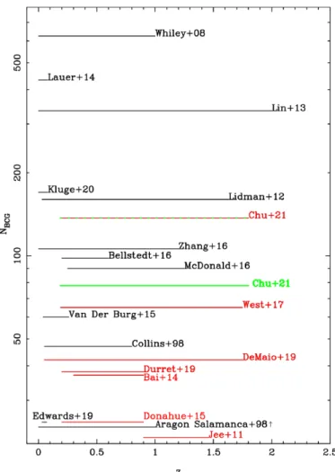
The present paper covers a large redshift range with one of the largest samples observed with HST (see Fig. 1, which is described in more detail in the next section). This will enable
Fig. 1.Comparison of the various samples of BCGs found in the liter-ature, considering the redshift range, the number of galaxies analyzed, and the type of data used. Only samples with at least 20 objects are represented here.Cerulo et al.(2019) with a sample of 74 275 BCGs is not represented here for reasons of legibility. The samples represented in black use ground-based telescope data, space-based data excluding HST, or a mix of ground-based and space-based data, while those in red only use HST data. Our initial sample is represented by the red and green dashed line, and our final BCG sample is in green (see Sect.4).
us to obtain more significant statistics on the evolution of BCG properties.
The paper is organized as follows. We describe the data in Sect.2, the method to automatically detect the BCGs in Sect.3, and the modeling of their luminosity profiles in Sect. 4. The results obtained as well as a short study of the link between the BCG masses, the distance between the BCG and the X-ray cen-ter of the cluscen-ter, and the physical properties are given in Sect.5. A final discussion and conclusions are presented in Sect.6.
Throughout this paper, we assume H0= 70 km s−1Mpc−1, ΩM= 0.3, and ΩΛ= 0.7. The scales and physical distances are computed using the astropy.coordinates package1. Unless
speci-fied, all magnitudes are given in the AB system.
2. Sample and data
2.1. Sample
The sample studied in this paper consists of 137 galaxy clusters with HST imaging taken from Jee et al. (2011),
Fig. 2.Histogram of the redshifts of the 149 BCGs in our sample. The red histogram shows all the BCGs studied, while the blue histogram (37 BCGs) shows those observed in rest frame filters that are too blue com-pared to the 4000 Å break (see Sect.3). The green histogram (25 BCGs) shows all BCGs with an important inner component (see Sect.4).
Postman et al.(2012a),Bai et al.(2014),Donahue et al.(2015),
West et al. (2017), DeMaio et al. (2019), Durret et al. (2019), andSazonova et al.(2020). We also add five more distant clus-ters at z ≥ 0.8, as well as the cluster Abell 2813 at z = 0.29. Among them, we identify 12 clusters that have in their center two BCGs similar in magnitude and size (see Sect.3). As a result, our final BCG sample contains 149 BCGs; the number of BCGs is not equal to the number of clusters studied because of the clus-ters with two BCGs. This sample is a good representation of the most massive BCGs in the range 0.1 ≤ z ≤ 1.80. The redshift distribution is shown in Fig.2.
All of these clusters have data available from the Hubble Space Telescope, obtained with the Advanced Camera for Sur-veys (ACS) in optical bands and/or the Wide Field Camera 3 (WFC3) in infrared bands, resulting in good-quality images. This allows us to perform accurate photometry with relatively good precision, and to treat all the BCGs in a homogeneous way. Contrary to other studies such asBai et al.(2014), we do not exclude from our study clusters with bright nearby objects that may hinder our measurements near the BCG area. We also identify in our sample two clusters that host blue BCGs (nega-tive rest frame blue-red color), with ac(nega-tive star forming regions inside the BCGs. These two BCGs will be described in more detail in Sect.3.
Our sample covers a large redshift range, which will enable us to trace the history of cluster formation through time. Figure1
shows the comparison of the sample sizes and redshift ranges between different studies done on BCGs2.Cerulo et al. (2019) studied a sample 74 275 BCGs from the SDSS in the redshift range 0.05 ≤ z ≤ 0.35, and is not represented in this figure for better legibility. Most large studies, especially those with HST data (represented in red), were done exclusively on local BCGs (z ≤ 0.1) (Lauer et al. 2014; Cerulo et al. 2019), while farther clusters and BCGs were limited to relatively small sam-ples (N ≤ 45) (Bai et al. 2014;DeMaio et al. 2019;Durret et al. 2019) and/or used ground-based data (represented in black). Our sample contains more clusters and BCGs at high redshifts (z ≥ 0.7) than that ofLidman et al.(2012) (73 and 33, respectively). 2 By increasing number of BCGs: Bai et al. (2014), Durret et al. (2019), DeMaio et al. (2019), van der Burg et al. (2015), West et al. (2017), McDonald et al. (2016), Bellstedt et al. (2016), Zhang et al. (2016), Lidman et al. (2012), Kluge et al. (2020), Lin et al. (2013), Lauer et al.(2014),Whiley et al.(2008), andCerulo et al.(2019).
With the present study, we therefore almost double the previ-ous samples and cover a larger range in redshift. This enables us to obtain more significant statistics on the evolution of BCG properties.
Lidman et al. (2012), Lin et al. (2013), West et al. (2017), andDe Propris et al. (2020) mainly focus on the alignment of BCGs with their host cluster and on the evolution of the BCG stellar masses. Our work constitutes a deeper analysis since we also study the luminosity profiles of the BCGs.
2.2. Retrieving data and cluster information
We retrieved all the FITS images from the Hubble Legacy Archive (HLA3). We looked for combined or mosaic images according to what is available, and downloaded stacked images directly from the HLA. To avoid handling such heavy files, we first cropped these images, defined the new center on the clus-ter coordinates found in NED, and created a new image that was 1.2 Mpc wide. Linear scales (arcsec Mpc−1) were deter-mined from the cluster redshifts in the literature (fromJee et al. 2011; Postman et al. 2012a; Bai et al. 2014; Donahue et al. 2015;West et al. 2017; DeMaio et al. 2019; Durret et al. 2019;
Sazonova et al. 2020, or were found in NED for the five other clusters we added). Cluster information can be found in Table1. It was necessary to add the keywords “GAIN” and “RDNOISE” in the header of the FITS images, to be used later by SExtractor or GALFIT. As the images are in units of electrons s−1, we set the GAIN to 1 and multiplied the images by the total exposure time (EXPTIME) to get back to units in electrons. Single exposure images were summed with AstroDrizzle to get the final com-bined images. We also retrieved the associated weight maps (wht fits) obtained applying the inverse variance map (IVM) option of AstroDrizzle.
3. Procedure for the detection of the BCG
The definition of the BCG that we use throughout this paper is the following. The BCG is the brightest galaxy in the cluster that lies close to the cluster center, defined as the center of the clus-ter member galaxy distribution. Generally, the clusclus-ter cenclus-ter is defined as the X-ray center of the cluster as X-rays trace the mass distribution better. However, it is difficult to obtain X-ray data, particularly at high redshifts. If a large sample is considered, most probably a good fraction of the clusters do not have X-ray data available. Moreover, it has been shown in several studies (Patel et al. 2006;Hashimoto et al. 2014;De Propris et al. 2020) that BCGs are often displaced from the X-ray center. For these reasons, and anticipating future works with much larger sam-ples, we use a definition that is independent from X-rays and only relies on optical and infrared photometric data. We define the center as that of the spatial distribution of cluster galaxies (as inKluge et al. 2020). X-ray coordinates are only available for 68 out of the 137 clusters in our sample (see Table4). These X-ray positions are only used to study whether or not the BCG proper-ties correlate with their position relative to the X-ray center (see Sect.5).
3.1. Method for detecting red BCGs
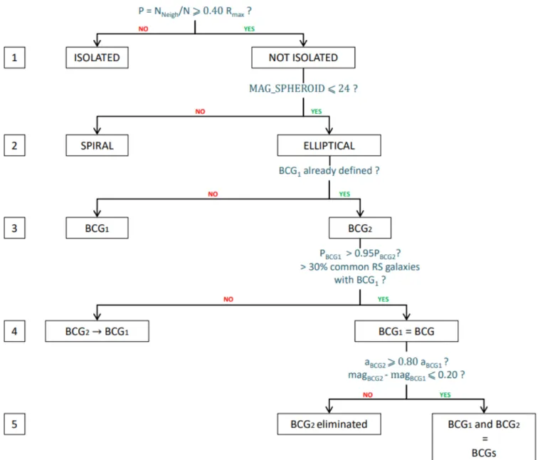
The method applied to automatically select red BCG is schemat-ically summarized in Fig.3, and is described in detail below. The
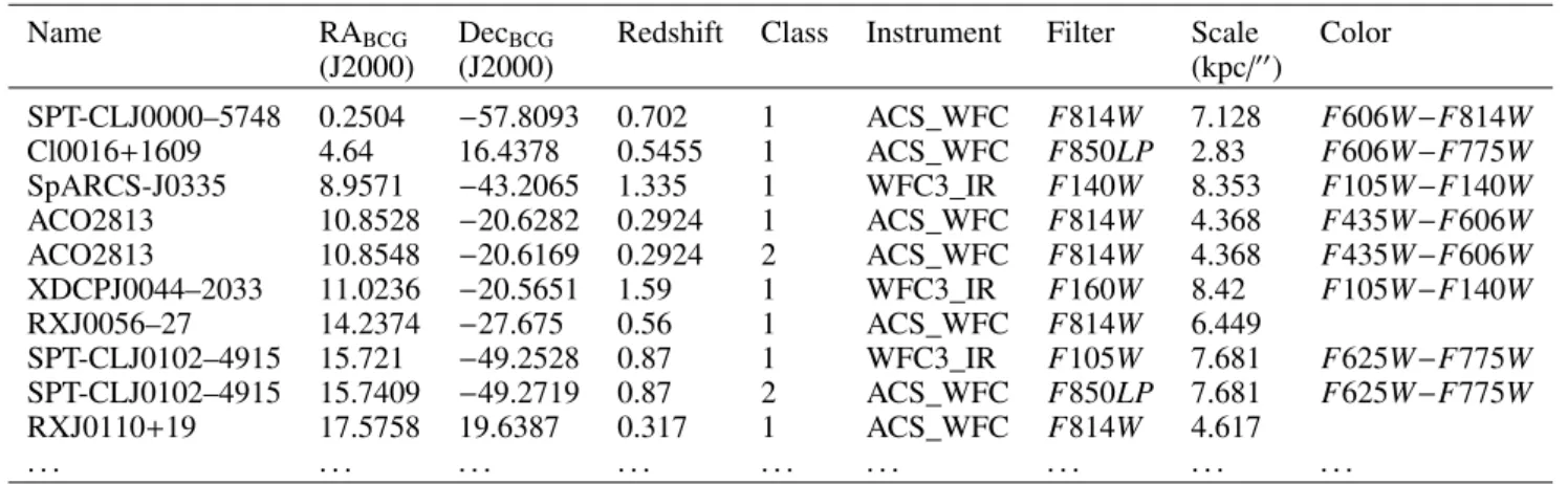
Table 1. Sample of the 149 BCGs studied in this paper.
Name RABCG DecBCG Redshift Class Instrument Filter Scale Color
(J2000) (J2000) (kpc/00) SPT-CLJ0000–5748 0.2504 −57.8093 0.702 1 ACS_WFC F814W 7.128 F606W−F814W Cl0016+1609 4.64 16.4378 0.5455 1 ACS_WFC F850LP 2.83 F606W−F775W SpARCS-J0335 8.9571 −43.2065 1.335 1 WFC3_IR F140W 8.353 F105W−F140W ACO2813 10.8528 −20.6282 0.2924 1 ACS_WFC F814W 4.368 F435W−F606W ACO2813 10.8548 −20.6169 0.2924 2 ACS_WFC F814W 4.368 F435W−F606W XDCPJ0044–2033 11.0236 −20.5651 1.59 1 WFC3_IR F160W 8.42 F105W−F140W RXJ0056–27 14.2374 −27.675 0.56 1 ACS_WFC F814W 6.449 SPT-CLJ0102–4915 15.721 −49.2528 0.87 1 WFC3_IR F105W 7.681 F625W−F775W SPT-CLJ0102–4915 15.7409 −49.2719 0.87 2 ACS_WFC F850LP 7.681 F625W−F775W RXJ0110+19 17.5758 19.6387 0.317 1 ACS_WFC F814W 4.617 . . . .
Notes. The columns are: full cluster name, coordinates of the BCG, redshift, class of the BCG (if two BCGs are defined for a cluster, class 1 represents the brighter of the two), instrument, filter used to model the luminosity profile of the BCG (see Sect.4), associated scale, color computed to extract the red sequence of the cluster (see Sect.3). The BCGs with no values in the last column only had data in one filter, and their coordinates were taken from the literature. The full table is available at the CDS.
efficiency of the method is discussed in Sect.3.1.4. Blue BCGs are mentioned in Sect.3.2.
3.1.1. Rejection of foreground sources
In order to differentiate the BCG from other objects in the field, we need to identify which objects are part of the cluster and which are not. We describe below our method for detecting the BCGs among all the contaminations (stars, foreground and back-ground galaxies, artifacts) in our images.
Measurements with SExtractor (seeBertin & Arnouts 1996, for more details on the parameters) were done using two di ffer-ent deblendings (parameters DEBLEND_MINCOUNT= 0.01 and DEBLEND_MINCOUNT= 0.02). The smallest deblending parameter (i.e., the finest deblending) is sufficient to separate two nearby galaxies without fragmenting excessively spiral galaxies in the foreground, and provides the most accurate measurements. However, BCGs can present a very diffuse and luminous halo which may be associated with ICL. We found that, in the pres-ence of nearby bright sources in the region of the BCG, SExtrac-tor would detect only those foreground sources and process the BCG halo as a very luminous background. We therefore decided to run SExtractor in parallel with a coarser deblending to take this into account. The two catalogs obtained with two di ffer-ent deblending parameters are then matched; we keep the val-ues obtained with the finer deblending, and add all new objects detected using a coarser deblending.
We computed the magnitude at which our catalog is com-plete at 80%, m80%. To achieve this we plot the histogram in apparent magnitudes and fit the distribution up to the magni-tude at which the distribution drops. By dividing the number of detected sources by the total number of sources expected to be detected in a magnitude bin (given by the fit), we compute the completeness of the catalog at each bin. We can then determine m80%, and make a cut in apparent magnitude to reject all galaxies with m ≥ m80%+ 2, as the photometry would not be accurate for these faintest objects.
Our procedure to reject the various contaminations is as fol-lows. First, we query in NED for all the sources in the region of the cluster and reject all those with a spectroscopic red-shift that differs by more than 0.15 from the cluster redshift (|z − zspec| > 0.15). We identify bad detections by their
mag-nitude values, which get returned as MAG= 99.99 by SExtrac-tor. All point sources or unresolved compact galaxies are elim-inated using the parameter CLASS_STAR ≥ 0.95 in SExtractor, which requires a point spread function (PSF) model to be fed into SExtractor, created with PSFex (Bertin 2011). Most foreground galaxies can be identified by their excessively bright absolute magnitude when computed from their MAG_AUTO magnitude and assuming they are at the cluster redshift. We thus exclude all sources with an absolute magnitude MAG_ABS ≤ −26.
We can identify edge-on spiral galaxies, which appear very elongated. They can be filtered by making cuts in elongation (defined in SExtractor as the ratio of the galaxy’s major to minor axis). As we explain in Sect.3.1.2, we consider two different
fil-ters. We define two different cuts depending on the filter we are looking at: in the bluest filter we apply the criterion ELONGA-TION ≤ 2.3, and in the reddest filter ELONGAELONGA-TION ≤ 2.6. The latter limit may seem quite high to filter efficiently all edge-on spiral galaxies. However, because of deblending issues, measur-ing with precision the lengths of the major and minor axes of the sources can be difficult, and will sometimes lead to a very elongated object. A very bright and elongated halo around the BCG, which can be linked to the ICL, will possibly return a high a/b axis ratio. This is the case for the BCG in RX J2129+0005, which has the highest a/b elongation (in the F606W filter) mea-sured in our sample, reaching a/b = 2.57 (see Fig.4). As the reddest filter is more sensitive to the ICL, we prefer to define a limit that is not too strict on this filter. It does not eliminate all edge-on galaxies (which would need a lower limit), but we can-not take the risk of filtering out any of the BCGs we are looking for. This is the reason why we define a different stricter limit on the bluest filter, as it is more sensitive to the blue stellar popula-tion present in the disk of spiral galaxies, and less to the ICL. 3.1.2. Selection of red cluster galaxies
Early-type galaxies in clusters are usually easily recognizable by their red color, since they are mostly red elliptical galaxies, with-out star formation. While blue spiral galaxies also exist inside the cluster, they are a minority, and red elliptical galaxies draw a red sequence in a color-magnitude diagram, which has a low disper-sion. We thus apply a filter in color in order to only keep the red galaxies that form the red sequence.
Fig. 3.Flowchart showing how BCGs are automatically selected, in the case of a rich cluster (see description of the method for our definition of a rich cluster). Values may change for less rich clusters (see Sect.3.1.3).
To extract all the red early-type galaxies in a cluster at redshift z, we model their color using a spectral energy dis-tribution (SED) template from Bruzual & Charlot (2003). The model is similar to the one used byHennig et al.(2017): a sin-gle period of star formation beginning at redshift zf= 5, with a Chabrier IMF and solar metallicity, that decreases exponen-tially with τ= 0.5 Gyr. However, it differs from theHennig et al.
(2017) model on the star formation redshift; we chose a higher zfto better model clusters at higher redshifts, whileHennig et al. (2017) limit their study to redshift z = 1.1. We reject all blue galaxies red ≤ 0) and all galaxies whose measured (blue-red) color differs by more than 0.60 mag from the model. While the red sequence of a cluster presents a rather narrow color-magnitude relation, and therefore very little dispersion, this large limit of 0.60 was fixed in order to take into account photo-metric uncertainties due to deblending issues, redshift uncer-tainties, or simply to the accuracy of the model used (Charlot, priv. comm.). The color is computed considering a fixed aper-ture of 35 kpc in diameter (parameter MAG_APER), which is large enough to contain all of the galaxy’s light. All magnitudes
are K-corrected (K-correction values from the EZGAL BC03 computed model), and we also take into account galactic extinc-tion. Dust maps were taken fromSchlegel et al.(1998), and red-dening values for the ACS and WFC3 bandpasses were taken fromSchlafly & Finkbeiner(2011), considering a reddening law RV= 3.1. The colors computed depend on the filters available and on the redshift of the cluster. The color computed for each cluster can be found in Table1.
The rest frame (blue-red) color to compute is defined as the color based on two magnitudes with the smallest wave-length difference that bracket the 4000 Å break at the cluster redshift. Depending on what filters are available for each clus-ter, the selected filters will differ. An example is given in Fig.5
for a cluster at z = 1.322; in this case the filters bracketing the 4000 Å break are F814W and F105W4. In the cases where the two optimal filters are not available, the color used to trace the red sequence galaxies at different redshifts may not be 4 The colors F606W−F625W and F775W−F814W were excluded as the two filters are very close to each other.
Fig. 4.BCG in RX J2129+0005 at redshift z = 0.234. The extended and luminous halo makes it difficult to accurately estimate the a/b axis ratio. In this case the major axis has most likely been overestimated, as the diffuse light is extended along this axis. The image was taken with the F775W ACS filter.
Fig. 5.SED of an elliptical galaxy from the CFHTLS (black solid line) redshifted at the cluster’s redshift (SPT-CL J0295–5829, z = 1.322). The filter transmissions are normalized to 1 for better visualization, and the break at 4000 Å is shown as a red vertical line for reference. In this case the chosen (blue-red) rest frame color is F814W−F105W, and the filter chosen for the final step (modeling the luminosity profile with GALFIT) is F140W (see Sect.4).
efficient; for instance, the use of the color (F606W−F140W) would not optimize the selection as a galaxy at higher redshift (z= 1.65 for example) than the cluster redshift (here z = 1.322) would have the same color and would not be filtered out. 3.1.3. Rejection of spiral and isolated galaxies
The cut in colors is an important step that allows us to remove most of the spiral galaxies and to maximize the number of ellip-ticals in our catalogs. However, a few foreground galaxies may still remain, and we describe here the method used to remove them.
The algorithm described hereafter is applied to every single galaxy, from the brightest to the faintest, until the cluster BCG is found. We refer the reader to the sketch shown in Fig.3. The procedure includes the following steps:
– Step 1: For each cluster we sort the catalog from the bright-est to the faintbright-est galaxies, and going down their brightnesses, we
Fig. 6. Histogram of the modeled bulge magnitudes (parameter MAG_SPHEROID) returned by SExtractor. All BCGs are shown in red; the blue bin represents a spiral galaxy close to the cluster ClG J1604+4304 (see Step 2).
exclude galaxies that are too isolated from the rest. We define the BCG as the brightest elliptical galaxy at the center of the galaxy density distribution. To calculate the center we compute NNeigh, the number of cluster members (i.e., red sequence galax-ies) found in a fixed aperture of 200 kpc radius centered on each galaxy in the final catalog, and note Nmax the maximum num-ber computed. If N is the total numnum-ber of red sequence galaxies whose colors fall within 0.60 mag from the model, and NNeigh is the number of neighbors of a given galaxy in an aperture of 200 kpc, we consider that a galaxy is isolated and unlikely to be the BCG if the ratio P = NNeigh/N is lower than 40% of Pmax= Nmax/N.
Considering that we cropped our images to cover a pro-jected area of 1.2 × 1.2 Mpc2, the aperture of diameter 400 kpc taken here represents one-third of the side of the images. This is small enough to detect high-density areas on the image, and big enough to work on clusters with a high spatial extent. After sev-eral trials adopting different values, the value of 200 kpc radius is the one that works best. Less than 200 kpc becomes too small for extended clusters, while a larger radius makes it difficult to detect the smaller density fluctuations, as the covered area becomes large. The limit defined at Rlim= 0.40 Rmaxwas also determined after several tests. This condition takes into account the cluster richness and spatial extent, as well as the possible offset of the BCG relatively to the cluster center.
– Step 2: The next step consists in filtering out the last spiral galaxies that remain among the potential BCG candi-dates. We run SExtractor to model the potential BCG with a bulge and a disk component. We find that spiral galaxies have a very faint bulge (parameter MAG_SPHEROID); as can be seen in Fig.6, a spiral galaxy (shown in blue) near the cluster ClG J1604+4304 prevented us from successfully detecting the BCG. We see a gap in magnitude between the spiral galaxy and the other BCGs (which are not all pure ellipticals). This enables us to define a new cut in magnitude to remove these remaining spirals: MAG_SPHEROID ≤ 24.
– Step 3: If a galaxy complies with these conditions (i.e., not being isolated and not being a spiral), we keep it as BCG1if no other BCG candidate was found before, and as BCG2otherwise. We do not proceed to the next step until a BCG2is defined.
– Step 4: We check if there are more red sequence members in the same aperture for BCG2than the number defined in Step 1 for BCG1by comparing their PNeighratios (defined in Step 1). We denote them PBCG1and PBCG2. If PBCG1≤ 0.95 PBCG2, and if
less than 30% of NNeigh,BCG2are in common with BCG1, BCG1 is eliminated and we define BCG2as the new BCG1.
The factor of 95% ensures that the overdensity in which BCG2 lies is significantly richer than the one in which BCG1 is. The second criterion on the number of galaxies common to BCG1and BCG2is to make sure that we are not replacing a BCG that is not at the very center of the cluster by another galaxy that is closer. This criterion is necessary to avoid eliminating BCGs that are a little offset from the center of the cluster where the den-sity is higher. It allows us to check that the two galaxies are not in the same area in the sky; in other words, we check that BCG2 does not belong to the same clump (overdensity) as BCG1, or that the two galaxies do not belong to the same cluster.
– Step 5: This step is taken only if BCG2 is defined, otherwise we repeat the previous steps until it is found. If BCG1 and BCG2 are similar in size (ratio of the major axes aBCG2/aBCG1≥ 0.80) and brightness (magnitude difference magBCG2–magBCG1≤ 0.2), we keep both BCG1and BCG2as the BCGs of the cluster. Otherwise, BCG2is eliminated and BCG1 is defined as the BCG.
The values above do not always work for poor clusters (i.e., when the number of cluster members is low or when the density of red sequence galaxies is low). There is no problem when all the cluster members are concentrated in the same area (with a size comparable to the previously defined aperture); however, if the members are dispersed over the sky and cover a large area, an aperture of 200 kpc radius becomes too small to detect den-sity fluctuations on the sky. We thus differentiate these clusters by their number of red sequence members, N, and by the previ-ously defined parameter Pmax(see Step 1). We separate the poor clusters with Pmax ≤ 0.25 and N ≤ 100 (very extended clusters with no important density clumps), and Pmax ≤ 0.5 and N ≤ 40 (low number of red sequence galaxies, extended spatial distri-bution). We were not able to correctly determine the BCGs for these clusters by defining a 200 kpc radius aperture, so for these poorer clusters, we consider a bigger aperture of 500 kpc radius. To take into account the bigger aperture, we also modify the sec-ond criterion in Step 4. We check that the two BCGs candidates, BCG1and BCG2, have less than 50% galaxies in common in the same aperture to guarantee that they are not both residing in the same cluster.
3.1.4. Results for detected red BCGs
Among the 137 clusters in our sample, 50 clusters only had one filter available, and were thus excluded from this procedure. For these 50 clusters without available colors, we visually checked the images to determine the BCG, and checked with X-ray maps or other studies before adding them to the final sample.
In order to assess the efficiency and accuracy of our detec-tion method, we checked each detecdetec-tion visually and compared it with other studies and with any X-ray map we could find. We compared the X-ray map to the position of the detected BCG to make sure that it is not too far from the X-ray peak (but not necessarily located at the peak, in a radius of about 200 kpc).
During this verification, we found that our detection dif-fers from that of Durret et al.(2019) and Bai et al.(2014) for the BCGs in MACS-J0717.5+3745 and SpARCS-J0224, respec-tively. MACS-J0717.5+3745 presents a very complex structure because is it undergoing multiple mergers (see Limousin et al. 2016; Ellien et al. 2019, and references therein). Durret et al.
(2019) define the BCG as the one in the southern structure; instead, we detected a brighter galaxy in the northern structure, which we define as the BCG. We decided to keep our detection
as it lies near the X-ray peak in the northern structure and is surrounded by galaxies at the cluster’s redshift. We found, by checking visually, that the BCG in SpARCS-J0224 defined in
Bai et al.(2014) is a spiral galaxy. We thus choose to keep our detection, which is an elliptical galaxy located just south of their detection.
A few star forming BCGs can be found in our sample. We find red BCGs with a very high star formation rate (SFR), for example MACS J0329.6–0211 at z = 0.45. This BCG has an almost starburst level of UV continuum and star formation (Donahue et al. 2015). Images of this BCG in the UV continuum and Hα–[NII] lines are given byFogarty et al.(2015), illustrat-ing the distribution of star formation throughout the galaxy. The high SFR of about 40 M yr−1 was confirmed byFogarty et al. (2017), based on Herschel data. Green et al. (2016) also indi-cate that this galaxy hosts an AGN, and is quite blue (blue-red= −0.71), with strong emission lines and a rather high X-ray luminosity of 11.85 × 1044erg s−1.
Overall, all the red BCGs, even those that are not pure ellip-tical BCGs or those with colors that are not optimized because of the lack of available filters, were successfully detected with our method. We successfully detect 97% of the BCGs in our sam-ple, and all the red BCGs are found. The method is effective in detecting red BCGs presenting different morphologies and char-acteristics (mergers, star forming, traces of dust in the core, dis-turbed).
It should be noted, however, that this method may be less reliable for poorer clusters (as defined in the previous sub-section). As we were conducting several tests, trying different values of apertures in which we computed the number of red sequence galaxies or the threshold below which galaxies are con-sidered isolated, we found that the detection efficiency for poorer clusters was more sensitive to these parameters. As this method relies on the density of red sequence galaxies in a small aper-ture, BCGs that are a little offset from the density peak (which is more difficult to calculate for poor clusters with an extended spatial distribution) could be eliminated, and rejected as being isolated from the other red sequence galaxies.
It is also important to note that, in the presence of more than one cluster (i.e., two clusters interacting with each other) or in the case of superclusters, only the brightest galaxy of one sub-structure will be detected. For MACS-J0717.5+3745 for exam-ple, the BCG of the northern clump is the brightest, and thus is the one detected by our algorithm.
3.2. Finding blue BCGs
Out of the 98 BCGs (87 clusters, 11 clusters with two BCGs) in our sample that we tried to detect, we find two peculiar BCGs with blue colors. Most brightest cluster galaxies are quiescent galaxies, and their dominant stellar population is typically red and old. As they grow by undergoing mergers through time, all their gas is consumed, and we expect the star formation to be quenched or suppressed. However, we do observe, both today and in the distant universe, BCGs with intense UV emitting fil-aments or knots, hinting at active star formation. Cerulo et al.
(2019) found that 9% of their sample of massive BCGs in the redshift range 0.05 ≤ z ≤ 0.35 from the SDSS and WISE sur-veys have blue colors (which they define as galaxies with colors 2σ bluer than the median color of the cluster red sequence), and are star forming. What we refer to from now on as star forming BCGs (SF BCGs), to date have only been observed in cool core clusters. Their morphology can be quite different from that of a simple elliptical galaxy, as was stated before. These galaxies can
Fig. 7.From left to right: MACS J0329–0211 (z= 0.45), an example of a red star forming BCG; RX J1532+3020 (z = 0.3615) and MACS J1932– 2635 (z= 0.352), the only two blue star forming BCGs in our sample.
appear disturbed, with a complex structure showing a possible recent or ongoing merger. Such examples of SF BCGs show that BCGs are not all simple ellipticals.
Two BCGs, RX J1532+3020 (z = 0.3615) and MACS J1932–2635 (z= 0.352), were not correctly detected as they are cool core BCGs with an extremely active star forming center, so they were eliminated because of their blue colors. These two BCGs were identified by eye and added manually, after check-ing and confirmcheck-ing with other studies. Their images are shown in Fig.7.
These two BCGs are the only blue BCGs in our sample (blue meaning a negative rest frame blue-red color) out of the 98 BCGs for which we compute a color. In comparison with other studies, we find a few other BCGs that are star forming but still red.
RX J1532+3020 is one of the most extreme cool core galaxy clusters observed today, as well as one of the most massive. An intensive study by Hlavacek-Larrondo et al. (2013) shows the existence of a western and an eastern cavity, which are used to quantify the AGN feedback at the center of the galaxy. These authors estimated that this feedback would release at least 1045erg s−1, which would prevent the intracluster medium (ICM) from cooling, and would then allow us to solve the cooling flow problem in cool core clusters. The BCG of this cluster is a radio loud galaxy that, in its central regions, presents UV filaments and knots, as well as traces of dust, hinting at recent star for-mation, with a SFR of at least 100 M yr−1 (Castignani et al.
2020). A strong and broad Lyman-α emission and stellar UV continuum, and no other emission lines, have been observed by
Donahue et al.(2016). CO with a large reservoir of molecular gas and with a high level of excitation have also been detected byCastignani et al.(2020).
MACS J1932–2635 is another cool core cluster with a huge reservoir of cold gas in the core, of mass (1.9 ± 0.3) × 1010M
, which makes it one of the largest reservoirs observed today, in whichFogarty et al.(2019) detected CO emission as well as UV knots and Hα filaments around the BCG. They measured a SFR of 250 M yr−1, and also observed an elongated tail that extends to the northwest, with traces of cold dust in the tail, which they suspect might be caused by a recent AGN outburst.
In order to detect these blue BCGs, we would have to relax the condition on the color. However, this condition is neces-sary in order to remove most of the spiral galaxies, and we find that allowing galaxies with blue colors would make the method much less reliable as the red sequence would be ill-defined. Our method is thus only reliable to detect red BCGs, even if they
are not pure ellipticals (star forming or merging galaxies, for example).
4. Luminosity profiles
We fit 2D analytical models on sources with GALFIT (Peng et al. 2002). Once the BCG is defined, we run SExtrac-tor one last time to return model fit parameters in the available filter closest to the F606W rest frame at redshift z (see Fig.5), which is at a wavelength above the 4000 Å break and thus in the spectral region where we get the highest flux. The chosen filters can be found in Table1. We note that there are 37 BCGs out of the 149 for which HST data are not available in the F606W rest frame or redder. The reddest filter is either bluer than the 4000 Å break or contains it, which means that not only are we looking at the oldest, reddest star population, but also at the youngest bluest stars. These BCGs are indicated by blue squares in the plots. The redshift distribution of all our BCGs is plotted in Fig.2; the blue histogram represents the clusters with filters which are bluer than the 4000 Å break. These clusters observed in filters that are too blue are mainly between redshifts 0.7 and 1.2.
4.1. Masking
We first need to mask all the neighboring sources. We take the SEGMENTATION map returned by SExtractor, and unmask the BCG (which is identified by an identification number), and also mask any blank region on the image. Because of deblending issues, it is more than likely that other objects, projected on the BCG, need to be masked.
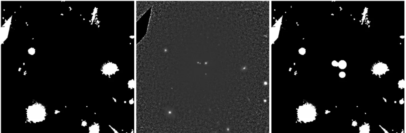
We use sharp divided images to detect any neighboring objects that pollute the signal. Sharp divided (SD) images (see e.g., Márquez et al. 1999, 2003) are obtained by dividing the images by the median filtered corresponding images. This brings out all the small neighboring sources that may have been hidden by the luminous halo of the BCG. We run SExtractor (again) on this SD image, and mask all the objects that are farther than 0.5 arcsec from the BCG coordinates (an example is given in Fig.8), which is the minimum distance required to avoid mask-ing the BCG center. As can be seen in Fig.8, the sources masked based on the SD image detection seem larger on the final mask than in the SD images, as the SD image does not show the true sizes of the objects. We apply a factor of 6 to the minor and major axes of the sources detected by SExtractor on the SD image to create our final mask. This factor allows us to include all the
Fig. 8.Example of the BCG in the cluster Abell 2261, at z= 0.224. Left: segmentation map returned by SExtractor, with the BCG unmasked. The pixels with a value of 1 are masked; those with a value of 0 are unmasked. Middle: sharp divided image in which four knots in the core appear. These knots were drowned in the light of the BCG and are now visible. Right: final mask (including the central objects).
luminosity of the sources and to mask them efficiently. If nec-essary, we identify by eye and draw the regions to be masked ourselves in SAOImage DS9 and create a new mask.
4.2. PSF model
To obtain a successful model of the galaxy profiles that also works for the inner regions, an accurate description of the PSF is needed. While the PSF we used for the photometry may have been sufficient to distinguish stars from galaxies, GALFIT requires the PSF to meet a number of criteria: it must have a very high S/N and a flat and zero background (otherwise any pattern in the background will appear on the model image when con-volved with the PSF); it should match the image (e.g., di ffrac-tion rings and spikes, speckle pattern); and it should be correctly centered (see GALFIT Technical FAQ).
We first subtract from the images the sky background, which is determined by masking all sources and blank areas on the clus-ter image, using the routine calc_background with a 3σ clip-ping method. We then use PSFex, and make a selective sam-ple of the stars that will go into making the PSF. We select all point-like sources with FLAGS= 0, MAG_AUTO ≤ 21, ELON-GATION ≤ 1.1, CLASS_STAR ≥ 0.98, S /N ≥ 20, and an isopho-tal print ISOAREA_IMAGE ≥ 20 pixels.
Since we work on HST observations that cover a small field of view, there may not be many bright stars in the field of the cluster that we could use to compute a PSF. We tried to take sev-eral faint stars and stack them to increase the S/N of the PSF. However, we find that this often results in a PSF with an uneven background that stands out during the model fitting returned by GALFIT, and this usually ends up being a bad fit (too large effective radius, large uncertainties). Since we are working on space observations, the PSF does not vary much, and though it may vary with time, the variations should not be significant (see
Martinet et al. 2017). This means that we can replace the PSF for a given filter by another one in the same filter with a better S/N. Higher S/N PSFs return better fits.
Modeled and theoretical PSFs are available for ACS/WFC and WFC3/IR. However, according to the GALFIT Technical FAQ5, the profiles obtained with models may not be realistic for space-based images, so we prefer to use observed PSFs.
5 https://users.obs.carnegiescience.edu/peng/work/
galfit/TFAQ.html
4.3. Profile fitting
We use GALFIT to fit two different models to our BCGs: a sin-gle Sérsic component or two Sérsic components, to allow di ffer-ent contributions from the inner and outer parts of the galaxies. We also tried to apply other models or combinations of mod-els including a de Vaucouleurs profile, but they always provided worse results (i.e., they gave a worse χ2, and about 30% of the BCGs were not well fitted with one or two de Vaucouleurs pro-files), so here we only discuss the results with Sérsic fittings.
It is necessary to give GALFIT an estimate of all the initial parameters: the effective surface brightness or total magnitude, the effective radius (the radius at which half of the total light of the galaxy is contained), and the elongation or the position angle (PA) of the BCG. These initial guesses are taken from the SExtractor catalogs: MU_EFF_MODEL
or MAG_AUTO, FLUX_RADIUS, ELONGATION, and
THETA_IMAGE. We did not have an estimate of the BCG Sérsic index, so we started from the value corresponding to the de Vaucouleurs profile: n = 4. If the fitting does not converge, we try different Sérsic indices in the range 0.5−10. For the second Sérsic component that accounts for the inner part, the following parameters are considered: MU_EFF_SPHEROID,
SPHEROID_REFF_IMAGE, SPHEROID_SERSICN, and
SPHEROID_THETA_IMAGE. The suffix SPHEROID refers to the bulb component when SExtractor tries to model a disk and a bulb to a galaxy. We consider an elongation (minor-to-major axis ratio, b/a) of 0.90 for the inner part, as an initial guess. The region to fit is a box that is 2.5 rKron wide (cf. GALFIT FAQ), rKronbeing the Kron radius returned by SExtractor. This is large enough to contain all the light from the BCG as well as some sky background, and is a good compromise to obtain good fits of our galaxies.
We first run GALFIT to fit the BCGs with one Sérsic com-ponent. If it does not manage to converge with a Sérsic index of n = 4, we try different values between 0.5 and 10 until it con-verges to a meaningful fit, and reject any fit with returned e ffec-tive radius larger than half the size of the fitting region, which is to say Re ≤ 2.5 rKron/2 pixels. We then use the output parame-ters as initial guesses to fit the outer part of the galaxy and add another Sérsic component to fit the inner part of the galaxy. If it does not converge towards meaningful values, we increment the Sérsic index until it manages to fit the BCG. For pairs of BCGs (two brightest cluster galaxies with similar sizes and mag-nitudes), we fit both of them simultaneously.
Fig. 9.Distribution of P-values as a function of redshift considering a model with one Sérsic component (magenta), and a model with two Sérsic components (cyan). BCGs that could not be fitted by either model are not included.
4.4. Choice of best fit model
The quality of the fit can be estimated from the reduced χ2 (χ2
ν), which should be close to 1. From our results we find that χ2
ν > 1.2 and χ2ν < 0.8 often indicate a bad fit. This happens when the model used to fit the BCG is not adapted, or when the initial parameters given are bad estimates. In this case, GALFIT may also not have converged and/or crashed. To decide whether a second component is really necessary to fit the BCG, or if one component gives equally good results, we use the F-test (Simard et al. 2011;Margalef-Bentabol et al. 2016). As stated in
Bai et al.(2014), as the background noise is not Gaussian, the meaning of χ2
ν is not as significant, and when comparing two models a χ2νcloser to unity does not necessarily mean that it is a better fit. So we prefer to use an F-test.
The test states that if the P-value, determined from the F-value and the number of degrees of freedom, is lower than a probability P0, then we can reject the null hypothesis and con-sider that the second model gives a significantly better result than the simpler one. The F-value is defined as the ratio of the reduced chi-squared values of the two models. GALFIT returns the χ2 and the χ2
νof the fit, but instead of directly considering the out-put χ2νcomputed by GALFIT, we compute χ2νas
χ2 ν=
χ2 nd.o.f.
(1) with nd.o.f. the number of degrees of freedom, which is defined here as the number of resolution elements, nres, minus the num-ber of free parameters in the model, nfree. nrescan be calculated as (seeSimard et al. 2011;Margalef-Bentabol et al. 2016) nres=
npixels
πθ2 , (2)
where npixelsis the number of unmasked pixels used for the fit-ting, and θ is the full width at half maximum (FWHM) of the given PSF in units of pixels, and nd.o.f.is then
nd.o.f.= nres− nfree− 1. (3)
The P-value is then calculated with the routine f.cdf from scipy.stats in python. We set P0 = 0.32, which represents a 1σ threshold value (Margalef, priv. comm.).
Fig. 10.Distribution of redshifts for each model: a single Sérsic com-ponent (magenta) and two Sérsic comcom-ponents (cyan). The overall distri-bution is shown in gray. The semi-filled histograms represent the initial sample, and the unfilled histograms only contain BCGs with appropriate data.
We show the distribution of P-values as a function of redshift in Fig.9. A P-value ≤ P0means that we need a second compo-nent to correctly model the BCG light distribution. We do not represent in this plot the BCGs that could not be fitted by either model: 9 BCGs could only be fitted with a single component, 22 could only be fitted with two components, 2 could only be fitted by fixing the Sérsic index n= 4 (de Vaucouleurs profile), and 2 BCGs could not be fitted or returned a poor fit for either of the models. In Fig.10it appears that BCGs that need a sec-ond component to obtain a good fit tend to be at lower redshifts (peak at z= 0.3), while the distribution for those that were well fitted with a single component is flatter. We also find BCGs with a model with two Sérsic profiles at higher redshifts (14 BCGs at z ≥ 1.0). If the chosen model depended on the distance, we would have expected not to have two component BCGs at higher z, which is not the case.
We must remember that part of our sample (37 BCGs) is studied in a too blue rest frame filter, and for these clusters we are not looking at the same star population. Without taking into account those observed in too blue filters, we find that 55 out of 72 BCGs (76%) at redshift z ≤ 0.8 need a second component, while the trend is reversed at z > 0.8, as 23 out of 38 BCGs (61%) can be nicely modeled with only one component. We also find that most of the BCGs observed with too blue filters (62%) can be modeled with only one Sérsic.
We also want to discover if the existence of these two dis-tinct populations (BCGs with two components at low z, and BCGs with a single component throughout redshift), with a limit around redshift z = 0.8, may be due to the fact that BCGs at higher redshifts are less resolved than their lower redshift coun-terparts. To test this hypothesis, we bring a sample of 44 BCGs at redshifts z ≤ 1.0 to a common physical scale at redshift z= 1.2. We smooth the images with a Gaussian and repeat the previous steps. The σgaussof the Gaussian to apply is calculated as σgauss= p(σ2z=1.2−σ
2 z,cluster)
with σz,clustercomputed from the FWHM of the image we want to degrade, and σz=1.2 the σ at the reference redshift z = 1.2, which was computed as
σz=1.2= σz,cluster∗
pixscalez=1.2 pixscalez,cluster
·
Of the 44 BCGs at z ≤ 1.0 on which we did this test, 30 returned results similar to those obtained with the original (unsmoothed) images. We also found that seven BCGs that were better fit-ted with two Sérsic components can be modeled just as well, according to the F-test, with only one Sérsic after smoothing the images. Surprisingly, the opposite also happened for seven other BCGs: four could not initially be fitted with two components and the other three were close to the P-value limit, Plim = 0.32. As 68% of the tested BCGs showed no significant difference, we can confirm that the lack of resolution for the farthest BCGs does not cause the absence of an inner component for BCGs at higher redshifts.
4.5. BCGs observed in too blue filters
In all that follows, when considering together the results from BCGs better fit with one or two Sérsic components, we con-sider the values obtained for the outer Sérsic component (Re,out≥ Re,in).
As stated before, we have 37 BCGs observed in too blue fil-ters (relative to the 4000 Å break). We must determine if they can be taken into account in our final study. For this, we run a test on 40 clusters with filters available on the blue side of the 4000 Å break as well as appropriate red filters, to check if the returned parameters vary depending on the filters chosen. We find that the absolute magnitude and mean effective surface brightness become fainter as the filter gets bluer. However, the dispersion is too big to simply correct for the offset to bring the BCGs observed in too blue filters to the appropriate red ones, perhaps because the filters on the blue side of the break do not always fall in the same spectral region on the SED (as the SED varies with redshift, and not all clusters were observed with the same filters). The effective radii can have their sizes halved when observed with too blue filters. As for the Sérsic indices, we find that the BCGs that need a second component tend to have Sér-sic indices in bluer filters consistent with those measured in the appropriate red filters. The BCGs which could be fitted with only one Sérsic have indices that vary without any clear pattern. These observations show that we cannot directly consider together the measurements obtained looking at different parts of the SED. Therefore, we chose to exclude the BCGs observed in too blue filters in what follows.
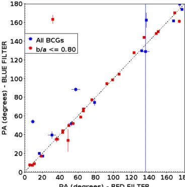
We find however that the position angles (PA) of the BCGs are not affected and remain consistent regardless of the filter cho-sen (see Fig. 11). The PAs of these BCGs will thus be kept. Only one point presents a big difference between the two val-ues (PAred–PAblue> 120◦). We found that the ICL associated with this BCG is more extended in the reddest filter; Ellien et al.
(2019), also show that the ICL tends to be more extended in red-der filters. The other BCGs with a significant difference between the values measured in the two different filters are circular in shape (b/a > 0.80), so the PAs are ill-defined, which also explains the huge error bars.
5. Results
As explained above, we tried fitting the BCGs with one or two Sérsic profiles. In the following the values plotted are those from the best model determined using the F-test (see previous section). The resulting parameters are summarized in Tables2
and3.
Fig. 11.PA measured in the appropriate red filter (x-axis), and measured in a too blue filter (y-axis). In red are BCGs with elongations b/a ≤ 0.80.
Two BCGs were not properly fitted by either model, but were correctly fitted by fixing the Sérsic index n= 4 (corresponding to a de Vaucouleurs profile). We thus kept the parameters obtained with this fit. Two other BCGs were not correctly fitted by either model, and were thus excluded, bringing our sample size to 147 BCGs.
We summarize the total number of galaxies that were fit with each model:
– Sérsic (1 component): 63 BCGs;
– Sérsic+ Sérsic (2 components): 84 BCGs.
Without taking into account the BCGs observed in too blue fil-ters we have:
– Sérsic (1 component): 40 BCGs;
– Sérsic+ Sérsic (2 components): 70 BCGs.
In all the plots shown in this paper, the BCGs better fitted with two Sérsic components will be represented with triangles, and those fitted with only one component with diamonds.
Before drawing conclusions, we need to know if we can con-sider together the results from BCGs better fit with one and with two Sérsic components. In principle, the two subsamples can be put together if, for the two components, we assume that the outer component contains most of the light of the BCG and that the outer profile represents well enough the overall luminosity of the galaxy. The more important the contribution of the inner compo-nent to the total luminosity of the BCG is, the less accurate this statement will be. If an inner component is required to model the BCG, then the resulting outer profile obtained when fitting two components may not be comparable to a profile obtained with only one component.
We show the histogram of the ratio of the inner compo-nent to total fluxes for the 70 BCGs requiring two Sérsic com-ponents (see Fig. 12), and find that 24 BCGs present a very important inner component, which can contribute up to 30% of the total luminosity of the galaxy. If we choose to ignore these 24 BCGs, no obvious difference can be seen in the overall
Table 2. Parameters obtained from fitting the luminosity profiles of the BCGs with GALFIT.
Name Class Model MABS hµei Re n b/a PA Alignment
(mag) (mag arcsec−2) (kpc) (degrees) (degrees)
SpARCS-J0335 1 Sérsic −26.088 25.034 57.488 8.7 0.88 158 4 XDCPJ0044–2033 1 Sérsic −25.073 23.119 12.944 3.39 0.36 11 63 CLJ0152–1357 1 Sérsic −24.859 23.471 21.802 3.59 0.7 49 CLJ015244.18–135715.84 2 Sérsic −24.378 22.698 12.74 4.24 0.75 42 CLJ015244.18–135715.84 1 Sérsic −24.478 22.343 11.331 7.96 1.0 10 RCSJ0220–0333 1 Sérsic −24.511 23.111 10.804 4.08 0.75 24 64 RCSJ0221–0321 1 Sérsic −23.916 22.257 5.667 0.88 0.61 111 63 RCSJ0221–0321 2 Sérsic −24.566 23.098 11.261 5.43 0.74 21 27 XLSSJ0223–0436 1 Sérsic −24.675 23.103 8.146 4.52 0.74 47 69 . . . . SPT-CLJ0000–5748 1 Sérsic2 −25.601 24.306 47.94 1.85 0.53 162 8 ACO2813 1 Sérsic2 −24.891 23.516 49.81 4.7 0.72 175 ACO2813 2 Sérsic2 −24.894 23.362 46.464 1.3 0.53 148 RXJ0056–27 1 Sérsic2 −24.641 23.613 28.883 1.83 0.64 94 SPT-CLJ0102–4915 1 Sérsic2 −24.87 22.478 13.894 1.62 0.87 118 29 SPT-CLJ0102–4915 2 Sérsic2 −25.753 22.069 15.653 1.26 0.57 134 13 RXJ0110+19 1 Sérsic2 −24.411 22.709 26.043 1.1 0.72 44 Abell209 1 Sérsic2 −24.327 21.734 19.715 2.05 0.71 134 23 SPT-CLJ0205–5829 1 Sérsic2 −25.701 26.197 82.853 1.09 0.33 32 8 XMMXCSJ022045.1–032555.0 1 Sérsic2 −24.403 21.638 16.486 2.34 0.91 65 . . . .
Notes. Only the parameters obtained for the chosen model are shown. If fitted by two Sérsic profiles, the parameters of the outer component are given (the parameters for the inner component are then given in Table3). The columns are: full cluster name, class of the galaxy, best model (Sérsic is a model with a single component, Sérsic2 is a model with two components, and Sérsic* fixes the Sérsic index n= 4), absolute magnitude, mean effective surface brightness, effective radius, Sérsic index, elongation (ratio of the major to minor axis), position angle, alignment of the BCG with its host cluster. The full table is available at the CDS.
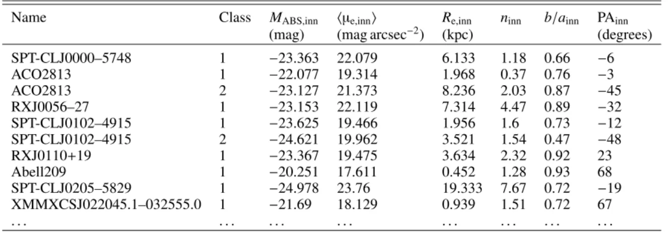
Table 3. Parameters obtained for the inner component, for BCGs fitted with two Sérsic profiles.
Name Class MABS,inn hµe,inni Re,inn ninn b/ainn PAinn
(mag) (mag arcsec−2) (kpc) (degrees)
SPT-CLJ0000–5748 1 −23.363 22.079 6.133 1.18 0.66 −6 ACO2813 1 −22.077 19.314 1.968 0.37 0.76 −3 ACO2813 2 −23.127 21.373 8.236 2.03 0.87 −45 RXJ0056–27 1 −23.153 22.119 7.314 4.47 0.89 −32 SPT-CLJ0102–4915 1 −23.625 19.466 1.956 1.6 0.73 −12 SPT-CLJ0102–4915 2 −24.621 19.962 3.521 1.54 0.47 −48 RXJ0110+19 1 −23.367 19.475 3.634 2.32 0.92 23 Abell209 1 −20.251 17.611 0.452 1.28 0.93 68 SPT-CLJ0205–5829 1 −24.978 23.76 19.333 7.67 0.72 −19 XMMXCSJ022045.1–032555.0 1 −21.69 18.129 0.939 1.51 0.72 67 . . . .
Notes. The columns are: full cluster name, class of the galaxy, absolute magnitude, mean effective surface brightness, effective radius, Sérsic index, elongation (ratio of the major to minor axis), position angle. The full table is available at the CDS.
relations observed in the following. However, we prefer to exclude them as the outer profile may not be comparable to the profile obtained with a single component modeling most of the light of the galaxy. After excluding the galaxies with a very bright inner component and those observed in too blue filters, we obtain the final numbers:
– Sérsic (1 component): 40 BCGs;
– Sérsic+ Sérsic (2 components): 46 BCGs.
In the following plots, BCGs observed in too blue filters are indi-cated by blue squares, and those fit with two Sérsic profiles and
with an important inner component are indicated by light pink squares. We also identify the blue SF BCGs (cf. Sect.3) with red squares and pairs of BCGs with black triangles.
5.1. Evolution with redshift
In order to study the evolution of the BCGs, we consider the dependence of the derived parameters as a function of redshift.
The absolute magnitudes of the BCGs, computed from the total apparent magnitudes (see Table1for the filters considered)
Fig. 12.Histogram of the ratio of the flux of the inner component to the total flux of the BCG, for clusters better fit with two components. Clusters observed in too blue filters are excluded in this plot.
calculated by GALFIT, despite the very big dispersion (4 mag thoughout redshift) tend to become brighter with redshift (see Fig. 13, left). The trend is faint, and can be quantified with a correlation coefficient R = −0.29 and a p-value p = 0.006563 (calculated from the coefficient R and the number of data points N6). By taking a significance level of α= 0.05, we show that we
can reject the null hypothesis (p < α) and conclude that the trend is significant.
There is a moderate trend for BCGs to grow with time (Fig.13, right), as those with the smallest effective radii are at higher redshifts (z ≥ 1.2). The trend in logarithmic scale is quan-tified by a correlation coefficient R = −0.40, and with a p-value of p = 0.000142. BCGs observed in too blue filters generally have smaller effective radii than the others at a given redshift. Those with an important inner component contribution do not appear to occupy a special place in these relations.
The mean effective surface brightness (Fig. 14) shows no significant evolution as a function of redshift (R 0.1), with a very large dispersion (spanning 6 mag at z ≥ 1.25). Seven BCGs at higher redshifts (z ≥ 1.4) can be seen among the galaxies with the brightest mean effective surface brightnesses (hµi ≤ 22 mag arcsec−2). We confirm that nothing peculiar was observed with these BCGs. Those observed in too blue filters and those with an important inner component contribution do not occupy a specific place in the relation.
The vertical gradient in color in Fig.14shows that the large dispersion is also linked to the effective radius. As we go towards the biggest BCGs (increasing effective radii), the relation is shifted towards the fainter mean effective surface brightnesses. This is to be linked with the Kormendy relation, which is shown in Sect.5.2.
Finally, there is no correlation between the Sérsic index and redshift (Fig.15, left). However, in the right panel, we see two different populations: the BCGs that were modeled with only one component generally have high Sérsic indices with a strong peak at n1comp,mean= 4 (without considering the BCGs observed in too blue filters), while the BCGs that were better modeled with two Sérsic components with lower Sérsic indices show a peak at n2comp,mean= 2.0.
5.2. Kormendy relation
The Kormendy relation (Kormendy 1977) links the (mean) e ffec-tive surface brightness of elliptical galaxies to their effective
6 https://www.socscistatistics.com/pvalues/
pearsondistribution.aspx
radius. This relation is plotted in Fig. 16. The different col-ors represent different redshift bins: z ≤ 0.3, 0.3 < z ≤ 0.5, 0.5 < z ≤ 0.9, 0.9 < z ≤ 1.3, and z > 1.3. We show that all the BCGs seem to follow the Kormendy relation with the same slope, but the ordinate at the origin of the line decreases with increasing redshift.
While applying a linear regression to the relation obtained in each redshift bin (R > 0.80, p < α), we find that the slope remains quite constant at all redshift bins, m = 3.33 ± 0.73, whereas the ordinate at the origin varies as c= 2.15 ∗ z + 16.65. 5.3. Inner component
The sample requiring an inner component consists of 46 BCGs. We find that the inner component follows a Kormendy rela-tion (Fig. 17), and is a continuation of the Kormendy relation shown in Fig.16at brighter mean effective surface brightness and smaller effective radius (Re,inn≤ 20 kpc).
We observe a very faint trend for the inner components to have brighter surface brightnesses with decreasing redshift, but the trend is not significant (R = 0.27, p = 0.06237 > α). We do not find any clear correlation (correlation coefficient ≤0.2) between redshift and the absolute magnitude, effective radius, or Sérsic indices of the inner component of the BCGs.
5.4. Alignment of the BCG with its host cluster
Some studies have shown that BCGs tend to have a similar ori-entation, or PA, to that of their host cluster (West et al. 2017;
Durret et al. 2019). As a comparison, we reproduce this study and compare our results with those of these two papers. The PA of the host clusters are taken fromWest et al.(2017) (computed from the moments of inertia of the distribution of red sequence galaxies) andDurret et al.(2019) (computed from density maps of red sequence galaxies), and the PAs of the BCGs are measured here with GALFIT. If measurements are given in both papers, the PAclusterinDurret et al.(2019) was used, unless the PAclusteris ill-defined (when the clusters are circular in shape), in which case the PA fromWest et al.(2017) was used. We did not measure the PA of the host clusters for the clusters that are not presented in the above-quoted papers as our images are not large enough to accurately measure the full extent and shape of the cluster.
We include all BCGs for which the PA of the cluster was measured (73 BCGs), including those observed with too blue fil-ters, as the PA measured by GALFIT is the same regardless of the filter (see Fig.11). We show the histogram of the alignment between the BCGs and their host clusters (defined as the di ffer-ence of PA between that of the cluster and the BCG) in Fig.18.
We find that 39 BCGs (53%) are aligned with their host clus-ter with a difference smaller than 30◦. This already shows a ten-dency for BCGs to align with their host clusters, as a random orientation of the BCGs would result in a flat distribution. BCGs with the highest PA difference tend to be circular in shape (elon-gation= b/a ≈ 1, for which it is more difficult to measure a PA, resulting in high uncertainties). We thus chose to exclude all BCGs with axis ratio b/a ≥ 0.8, in order to eliminate BCGs with ill-defined PAs, as shown in red in the histogram. We then find that 32 out of 58 of BCGs are aligned with their host cluster within 30◦, slightly increasing the percentage to 55%. There is a secondary peak between a PA difference of 30 to 40◦, mainly corresponding to BCGs at redshift z ≥ 0.9. At such high red-shifts, galaxies appear smaller, and therefore the accuracy of the measured PA is probably worse. If we only consider galaxies at z ≤0.9 (blue histogram), we find that 22 BCGs out of 30 (73%)
Fig. 13.Left: absolute magnitude and Right: effective radius in logarithmic scale as a function of redshift. Cyan triangles are BCGs fit by two Sérsic components (the outer component is considered), while the magenta points are BCGs fit with only one Sérsic component. Blue squares represent the BCGs observed in too blue filters, red squares are SF BCGs (see Sect.3), black triangles are pairs of BCGs, and the light pink squares are BCGs with an important inner component contribution.
Fig. 14. Mean effective surface brightness as a function of redshift (color-coding as in Fig. 13). Additional information on the effective radii of the BCGs is shown on the right of the figure.
align with their cluster within less than 30◦. This shows that most BCGs tend to align with their host cluster at least at z ≤ 0.9. 5.5. BCG physical properties as a function of host cluster
properties
We browsed the available bibliography to retrieve the cluster masses and X-ray center coordinates. The corresponding data can be found in Table4. We preferred lensing-based mass esti-mates if they were available. We brought all the masses to M200, applying the conversion factor between M500 and M200: M500= 0.72 M200(Pierpaoli et al. 2003).
We show the richness of the cluster as a function of redshift and cluster mass in Fig. 19. The richness N of the cluster is defined here as the number of red sequence galaxies (found in Sect. 3) in an aperture of 500 kpc radius around the BCG. We obtain different values of N for two different BCGs in the same cluster because the richness is computed in an aperture centered on each BCG.
As can be seen in Fig. 19 (left panel), clusters seem to become richer with decreasing redshift (correlation coefficient
in logarithmic scale R= −0.70 and p-value of p < 10−5). Clus-ters at higher redshifts (z ≥ 1.0) have a lower richness, with a number of detected red sequence galaxies N ≤ 60. The right panel also shows that the most massive clusters are also the rich-est, and the high-redshift clusters (blue points on the plot) with a low richness are also the least massive (M200,c≤ 5 × 10¹⁴M ). This low value of N could in principle be due to the depth of our images as we have a bias due to the distance: at higher redshifts it is more difficult to detect objects, and only the brightest ones can show up.
However, when looking at Fig.20, the left panel shows that we do not observe very massive clusters at high redshifts. So we have no bias due to the distance of the galaxies when mea-suring cluster masses: the masses are measured via lensing or derived from X-ray or SZ maps, which are independent of dis-tance. Thus, we conclude that clusters become richer with time, and this result is not due to the depth of our images. However, although we only observe very massive clusters at lower red-shifts (M200,c ≥ 30 × 1014M at z ≤ 0.8), the masses of the clusters do not vary much with time (R < 0.20). The right panel shows that the very massive clusters only host bigger BCGs: clusters with masses M200,c ≥ 25 × 1014M only have BCGs with effective radii Re≥ 30 kpc. We find no correlation (R ≤ 0.2) between the BCG surface brightnesses or Sérsic indices and the cluster masses.
Using the relation given inBai et al.(2014), we compute an estimate of the BCG masses from the cluster masses: M∗
BCG ∝ M0.6
cluster. We find that the most massive BCGs are also the biggest (moderate correlation with R= 0.46 and p = 0.00007) and also tend to be brighter (R = −0.32, p = 007353). No correlation between the BCGs masses and redshift is seen (R < 0.20).
We also study how the BCGs behave depending on their o ff-sets to the cluster X-ray center. We exclude superclusters and clusters that present several substructures and/or several BCGs. We show the histogram of the offsets in Fig.21, top left panel. We find that 31 out of 61 (51%) are within a 30 kpc radius range from the X-ray center of the cluster, showing that BCGs tend to lie close to the cluster X-ray centers. The two star forming BCGs that have undergone recent mergers and are not at equilibrium are also located at the center of the cluster (DX ≤ 10 kpc). We confirm, however, that there can be a significant offset between the two: 12 out of 61 BCGs (20%) present an offset bigger than 100 kpc. Although the corresponding plots are not shown here,