HAL Id: hal-00299510
https://hal.archives-ouvertes.fr/hal-00299510
Submitted on 11 Apr 2008
HAL is a multi-disciplinary open access
archive for the deposit and dissemination of
sci-entific research documents, whether they are
pub-lished or not. The documents may come from
teaching and research institutions in France or
abroad, or from public or private research centers.
L’archive ouverte pluridisciplinaire HAL, est
destinée au dépôt et à la diffusion de documents
scientifiques de niveau recherche, publiés ou non,
émanant des établissements d’enseignement et de
recherche français ou étrangers, des laboratoires
publics ou privés.
deformation monitoring networks
E. Tanir, K. Felsenstein, M. Yalcinkaya
To cite this version:
E. Tanir, K. Felsenstein, M. Yalcinkaya. Using Bayesian methods for the parameter estimation of
de-formation monitoring networks. Natural Hazards and Earth System Science, Copernicus Publications
on behalf of the European Geosciences Union, 2008, 8 (2), pp.335-347. �hal-00299510�
www.nat-hazards-earth-syst-sci.net/8/335/2008/ © Author(s) 2008. This work is distributed under the Creative Commons Attribution 3.0 License.
and Earth
System Sciences
Using Bayesian methods for the parameter estimation of
deformation monitoring networks
E. Tanir1,2, K. Felsenstein3, and M. Yalcinkaya2
1Vienna University of Technology, Institute of Geodesy and Geophysics, 1040 Vienna, Austria
2Karadeniz Technical University, Department of Geodesy and Photogrammetry Engineering, 61080 Trabzon, Turkey 3Vienna University of Technology, Institute of Statistics and Probability Theory, 1040 Vienna, Austria
Received: 24 October 2007 – Revised: 25 January 2008 – Accepted: 27 March 2008 – Published: 11 April 2008
Abstract. In order to investigate the deformations of an area
or an object, geodetic observations are repeated at differ-ent time epochs and then these observations of each period are adjusted independently. From the coordinate differences between the epochs the input parameters of a deformation model are estimated. The decision about the deformation is given by appropriate models using the parameter estimation results from each observation period. So, we have to be sure that we use accurately taken observations (assessing the qual-ity of observations) and that we also use an appropriate math-ematical model for both adjustment of period measurements and for the deformation modelling (Caspary, 2000). All in-accuracies of the model, especially systematic and gross er-rors in the observations, as well as incorrectly evaluated a priori variances will contaminate the results and lead to ap-parent deformations. Therefore, it is of prime importance to employ all known methods which can contribute to the de-velopment of a realistic model. In Albertella et al. (2005), a new testing procedure from Bayesian point of view in defor-mation analysis was developed by taking into consideration prior information about the displacements in case estimated displacements are small w.r.t. (with respect to) measurement precision.
Within our study, we want to introduce additional parame-ter estimation from the Bayesian point of view for a deforma-tion monitoring network which is constructed for landslide monitoring in Macka in the province of Trabzon in north eastern Turkey. We used LSQ parameter estimation results to set up prior information for this additional parameter es-timation procedure. The Bayesian inference allows evaluat-ing the probability of an event by available prior evidences and collected observations. Bayes theorem underlines that the observations modify through the likelihood function the
Correspondence to: E. Tanir ([email protected])
prior knowledge of the parameters, thus leading to the poste-rior density function of the parameters themselves.
1 Introduction
The technological progress during the last decades has also affected geosciences and the observational methods in all fields of geosciences have changed gradually. Therefore, to-day measurements for deformation monitoring are conducted commonly by satellite based techniques. Consequently, it becomes possible to make deformation monitoring studies in adequate accuracy in less time for larger areas. However, the increasing observational accuracy requires adequate mathe-matical and statistical models. Measurement errors occur no matter how measurements are taken by terrestrial and satel-lite techniques and have to be eliminated from the measure-ments. Determining measurement errors by effective mea-surement analysis is as important in deformation monitoring studies as determining the deformation model itself. In the last decade, attention has shifted towards Bayesian statistics, which has advantages in complex problems and better re-flects the way scientists think about evidence. Recently, the Bayesian statistics has been used efficiently in the areas of engineering, social sciences and medicine (Koch 1990; Yal-cinkaya and Tanir, 2003).
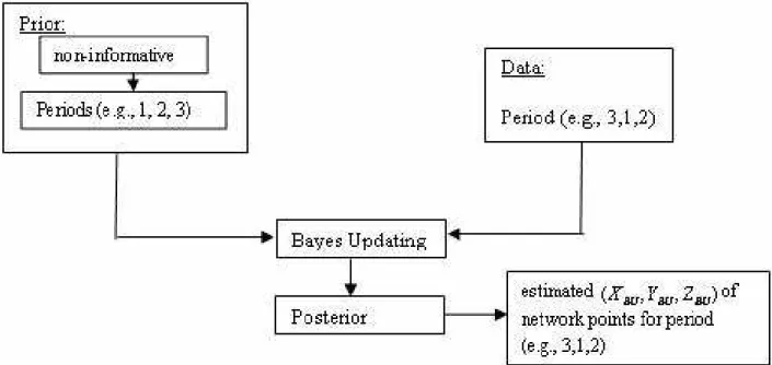
Bayes theorem leads to posterior distribution of unknown parameters given by the data. All inferential problems con-cerning the parameters can be solved by means of poste-rior distributions. Based on these distributions we will es-timate the unknown parameters, establish confidence regions for them and test hypotheses concerning the parameters. In this study, it is aimed to apply Bayes-Updating (BU) and Gibbs-Sampling (GS) algorithms in a geodetic parameter es-timation problem. In addition, the task is to inform the user which algorithm is more useful in the aspect of accuracy and
methodology. We investigated the sensitivity of these algo-rithms due to the use of different prior information.
To apply the Bayes-Updating we introduce the prior in-formation for station coordinates. We started up with non-informative prior and used different epoch observations in different order to stepwisely update prior information. In Gibbs-Sampling algorithm we introduce different starting points w.r.t. point positioning errors. Usually, measure-ments at different points of a network are of different ity concerning their statistical variance. We test the qual-ity of network points estimated coordinates by comparing the Bayesian estimates derived from a Bayes-Updating (con-jugate updating) algorithm or a Gibbs-sampling procedure. The total variation (L1-distance) of the resulting estimates serves as measure of discrepancy for reasons of robustness. The information contained in a network point is evaluated by taking that point as starting point for Gibbs-sampling. The distances (L1-measure) between Bayesian updating and Gibbs-sampling indicate how much imprecision the point adds to the estimation procedure.
We consider the information contained in different data sets as well as the influence of one single network point. The differences of estimation taking data sets in exchanging or-der (concerning prior data set and actual data set) serves as method to evaluate the information contained in the data set.
2 Bayesian parameter estimation methods
2.1 Bayes updating
The basic instrument of Bayesian procedures consists of the updating algorithm via Bayes theorem
π(θ|D) ∝ l(θ, D)π(θ) (1) where π(θ ) denotes the prior distribution and π(θ|D) the posterior distribution of the model parameter. l(θ, D) de-notes the likelihood function of the data. For the network data we use a correlated normal vector y with the mean vec-tor µ and variance-covariance matrix 6. In a conjugate prior approach the prior knowledge about parameters is assessed in the same form as the likelihood. In case of correlated normal observations the corresponding prior is a Normal-Wishart distribution (Felsenstein, 1996). The common prior of µ and the precision matrix P=6−1is split into a normal part as a normal distribution with a mean of m and standard deviation of (bP)−1
µ/P∼ N(m, (bP)−1) (2) with b>0 and Wishart part
P=6−1∼ Wis(a, 3) (3) The weights b, a>0 play the same role as the number of observations in the likelihood. µ is the prior guess for the
mean and 3 a prior guess for the covariance matrix. For the data of the geometric network it is important to specify the prior covariance according to the geometric structure (Eu-clidian distances on surfaces). Once the prior hyper param-eters are specified the posterior can be achieved through the updating of the hyper parameters only. The posterior density is
π(µ, P|D)=f (D|µ, P)π(µ|P)π(P)
m(D) (4)
where f denotes the multivariate Normal distribution with mean µ and precision matrix P. The marginal density is
m(D)= Z
f (D|µ, P)π(µ|P)π(P)dµdP (5) For more details see also Rowe 2002. The hyper parame-ters are computed out of data vectors as following by
m∗= bmb + n ¯y + n (6) and 3∗= 3 + nb b+ n(m− y)(m − y) T + R (7)
where R is the empirical covariance
R=X
i
yiyTi − nyy
T (8)
The Eqs. (6), (7) and (8) are considered as updating algo-rithm for current epoch of a geodetic network with a priori data set of the same network from a different epoch with m∗ posterior mean for current data epoch, b number of obser-vations of different epochs which prior information comes from, m observations’ prior mean of different epochs which prior information comes from, n number of observations of current epoch. 3 variance-covariance matrix of observations of different epoch which prior information comes from, 3∗ posterior variance-covariance matrix of observations of cur-rent epoch. The modelling through a conjugate family of pri-ors is indeed attractive even in case of little informative prior information. Prior distributions carrying as little information as possible can be considered as limits of conjugate priors in the sense
3→ 0 (9)
and b→0. The conjugate property is not restricted to a sin-gle distribution. Mixtures of Normal-Wisharts are conjugate as well allowing more flexibility to the model. For weighting we choose several values of b in our calculations to analyze the sensitivity of the estimates upon the prior distributions (Robert, 2001). Bayesian estimates of the different parame-ters of the network are calculated as posterior means leading to weighted mixtures of the means
m∗j = bmj+ ny
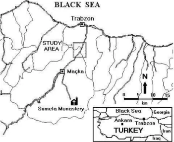
Fig. 1. Location map of study area (Yalcinkaya and Bayrak, 2003).
as the posterior expectations of µ. Here j indicates one Normal-Wishart distribution out of the mixture. aj and bj are altered according to a∗=a+n and b∗=b+n. The
Bayesian estimate of the covariance is
E(6/D)= 1
a+ n − k − 13
∗ (11)
where k is the dimension (k=14, number of network points in this study). Since the specification of a completely infor-mative prior turns out to be practically impossible for the co-variance structure we choose an approach which can be com-pared to a modified empirical Bayes setup. First we take one data set as a learning sample equipped with non-informative prior. By this first step we achieve a reliable prior guess of 6 used as 3. Namely, we insert the empirical covariance matrix of the learning sample as prior covariance matrix. In alternat-ing these startalternat-ing sets and comparalternat-ing the results we analyze the sensitivity of the model concerning the prior covariance structure. Note that Bayesian estimates coincide with stan-dard least-squares estimates in case of non-informative pri-ors.
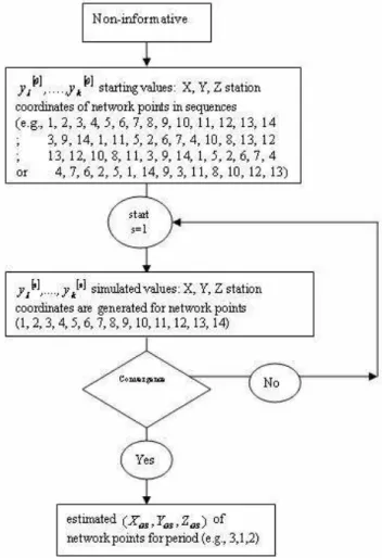
2.2 Gibbs-sampling
Since all measurements in the network are highly correlated the distributions (posterior as well as prior) of the parameters become high dimensional. Therefore an algorithm is needed to handle the posterior distributions which incorporate the special covariance structure of the data. The generic Gibbs algorithm aims at reproducing the posterior density and as-sociated estimates in an automatic manner. Gibbs sampling represents a specific application of general MCMC (Markov Chain Monte Carlo) processes (Robert and Casella, 2004).
The Gibbs sampling algorithm works as follows. The distribution of the k dimensional stochastic variable
Fig. 2. 3D-view of the study area.
y=(y1, ...., yk) is simulated by the following transition from
step s to s+1. The basic idea of the algorithm is the sim-ulation of the full conditional distributions where the com-ponents of the stochastic vector are replaced in turn. Let
y1[0], ...., yk[0]denote a proper starting value for network point coordinates and y1[s], ...., yk[s]the result of the sth step. The components of y1[s+1], ...., yk[s+1]are generated according the conditional distributions D,
Z1∼D(Z/y2[s], ...., yk[s]) Z2∼D(Z/Z1, y3[s], ...., yk[s]) (12)
The iteration for the kth component
reads Zk∼D(Z/Z1, ...Zk−1). The vector
(Z1, ...., Zk)=(y1[s+1], ...yk[s+1]) serves as realization
in the s + 1th step. The conditional distributions are one dimensional and therefore the algorithm does not change in structure if k increases. While working with normal distributions, a data augmentation leads to conditionally independent variables. That ensures several convergence properties of the procedure as well.
In our network we introduced non-informative priors. These priors are based on the Fisher information and are not normalized. The conditional distributions can be obtained di-rectly by the Gibbs sampler if we start the procedure within a certain region. Standard arguments of convergence of the Gibbs sampler fail in the case of non-informative priors. A monitoring of the simulation and the corresponding estimates is needed and we choose with this problem by using data sets as training samples. Therefore we reach a state of the proce-dure where a proper prior is given.
If the Bayesian estimate of the parameter is needed only instead of the complete posterior distribution a version of Gibbs sampling is carried out for computing the parameter estimates. Such algorithms are called EM-algorithm (Expec-tation Maximization) and are originally introduced to calcu-late maximum likelihood estimates. The stepwise calcula-tion of a maximum likelihood estimate involves the cyclic
Fig. 3. Flowchart for BU method.
exchange of the parameters as in the above calculation com-bined with a maximization step (Felsenstein, 2001). If the prior distribution is non-informative maximum likelihood and Bayes estimation coincide for normally distributed data. The results of Bayesian estimates reduce to the calculation of the least square estimates if non-informative priors are used only.
3 Application
3.1 Information about the study area and individual adjust-ment results for different periods
Earthquakes and landslides are two most effective natural hazards in Turkey. The Eastern Black Sea region of Turkey receives a lot of rainfall and experienced very heavy flooding ( ¨Onalp, 1991; Tarhan, 1991; Ocakoglu et al., 2002). This gion undergoes much more landslides compared to other re-gions of Turkey. Landslides on this region of Turkey damage agricultural areas, railways and cause the loss of life. Be-cause of these reasons, scientists put this region as one of the most priority areas for their research. We selected Kut-lug¨un Village in Macka County in the Province of Trabzon in Eastern Black Sea Region of Turkey as study area (Fig. 1). Kutlug¨un landslides damaged the Trabzon-Macka Highway and the Water Pipe Line supplying drinking water to Trab-zon city-centre. Besides, lots of residential estates were af-fected during slow sliding. In order to prevent possible fu-ture damages of landslides at Kutlug¨un village, a geodetic deformation network was established in the year 2000 for landslide monitoring within the project of “Determination
of landslides by dynamic models” by researchers from the Department of Geodesy and Photogrammetry Engineering at Karadeniz Technical University. In this study, repeated GPS surveys at certain time periods, belonging to a geodetic de-formation network in Macka in the province of Trabzon in north eastern Turkey (Fig. 1) are used.
The network consists of 14 points, with four of them (2, 8, 10, and 13) on solid ground. The other points (1, 3, 4, 5, 6, 7, 9, 11, 12, and 14) were placed into moving mate-rial (Fig. 2). All of them were built with pillars. Geodetic deformation measurements were made in November 2000, February 2001 and May 2001 with Ashtech GPS receivers in a static mode. This data was evaluated by Geogenius-2000 software. The outputs of this software are baselines (l) be-tween network points and cofactor matrices of each baseline
(Q) which were used also as input data in the studies of
Yal-cinkaya and Bayrak, 2003, 2005. With these outputs from the GPS software and approximate coordinates for network points, we can write our observation equations in the Gauss Markov Model (GMM) to estimate network point positions by least-squares estimation. The results from least-squares estimation are used as input data for Bayes-Updating and Gibbs-Sampling algorithms in this study.
The GMM is a linear mathematical model consisting of functional and stochastic relations. It relates observations to parameters. In matrix notation it takes the following form
E(l)= Ax l= Ax + ε (13)
E(εεT)= 6 = σ02Q (14) where l is the n×1 vector of observations, E(.) is expecta-tion operator, A is the n×3u matrix of known coefficients, ε
is the n×1 vector of errors, x is the 3u×1 vector of unknown parameters, 6 is the n×n covariance-covariance matrix, Q is the n×n cofactor matrix of observations with u number of network points and n number of baselines. σ02is a priori variance factor. This theoretical model is rewritten to esti-mate parameters (network station coordinates) from real data (baselines between network points) in the following form
l+ v = A ˆx P= Q−1 (15) where P is the n×n weight matrix of observations; v is the n×1 vector of residuals. The estimation function
ˆx=(ATPA)−1(ATPl) is used to get the estimated values of
network point coordinates (see Table 1).
mp(i)=qm2x(i)+m2y(i)+m2z(i) with (i=1, 2, ..., u) number point positioning error for network points are calculated by Qxx=(ATPA)−1 as u×u cofactor matrix of estimated
parameters, Kxx=σ2Qxxu×u variance-covariance matrix
of the estimated parameters and m(xyz)i=√(Kxx)ii with (i=1, 2, ..., u) mean-square errors for estimated coordinates.
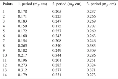
By looking at the mp(i) values of points, three different
groups in each period are determined as accurate, more ac-curate and the most acac-curate. The starting points are se-lected from these groups. I.e., point 4 can be assigned to the first group with the smallest mpvalue, point 3 to the
sec-ond group, and point 13 to the third group with nearly the biggest mp value at every period. The grey rows in Table 2
are used to express the points which are selected as starting points according to their mp(i)values. The starting points are
selected as 1, 3, 4, and 13 (see Table 2). Different point se-quences which are constructed according to such a grouping for network points are used for Gibbs Sampling algorithm later.
3.2 Comparison between different bayes updating and gibbs sampling algorithms
The parameter estimation with Gibbs-Sampling is applied with different starting points and with Bayes updating with different prior information (Roberts and Rosenthal, 1998). The results obtained with different information (starting points and prior information) in two different algorithms are compared. Coordinate parameters estimated from Gibbs-Sampling (GS) algorithm and Bayes-Updating (BU) are called as (XGS, YGS, ZGS) and (XBU, YBU, ZBU). Figures 3
and 4 show flowcharts of BU and GS methods respectively. Parameters of the differences are calculated; one is the dif-ference between Bayes-Updating and Gibbs-Sampling algo-rithms (BU-GS), one is between Gibbs-Sampling algoalgo-rithms and the other is Bayes-Updating algorithms. These differ-ences are calculated as
Fig. 4. Flowchart for GS method.
(BU GS)n=
q
(XBU(j)−XGS(i))2n+(YBU(j)−YGS(i))2n+(ZBU(j)−ZGS(i))2n
(GS)n=
q
(XGS(i)−XGS(k))2n+(YGS(i)−YGS(k))2n+(ZGS(i)−ZGS(k))2n
(BU)n=
q
(XBU(j)−XBU(l))2n+(YBU(j)−YBU(l))2n+(ZBU(j)−ZBU(l))2n (16)
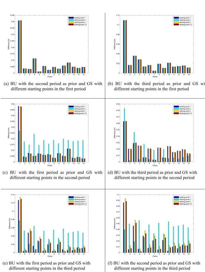
Here, i and k indicate the starting points in Gibbs-Sampling algorithm (e.g., 1, 3, 4, or 13); j and l indicate prior information (e.g., the first, second or third period) and n indicates the number of points in the network. The re-sults are drawn (in Figs. 5 and 6) except for GS. Compar-isons are made by using different types of prior informa-tion in Bayes updating and taking different starting points (4, 3, 13) in Gibbs-Sampling algorithm. For a compari-son between the different algorithms, the smoothness pa-rameters (VR) are calculated on values of different algo-rithms. f (1), f (2), ..., f (n) values are taken as (BU GS) and (BU ) values and (VR) values for all plots are calculated from VR=Pni=2|f (i)−f (i − 1)|.
For the first period, the differences on all points are ap-proximately the same except of point 1 (see Table 3). Be-cause the VR values are nearly the same as for all situations,
(a) BU with the second period as prior and GS with different starting points in the first period
(b) BU with the third period as prior and GS with different starting points in the first period
(c) BU with the first period as prior and GS with different starting points in the second period
(d) BU with the third period as prior and GS with different starting points in the second period
(e) BU with the first period as prior and GS with different starting points in the third period
(f) BU with the second period as prior and GS with different starting points in the third period
Figure 5. Differences between BU and GS Results
Table 1. Adjusted station coordinates for each period. No X(m) Y (m) Z(m) November 2000 (1. period) 1 3710656.9536 3083935.0997 4157818.3179 2 3710501.7100 3084005.1000 4157907.9599 3 3710542.0823 3084033.1843 4157788.0178 4 3710709.5387 3084028.6271 4157648.6440 5 3710480.9725 3084117.3939 4157741.7704 6 3710274.8591 3084218.3811 4157799.2949 7 3710479.6401 3084171.0299 4157677.5811 8 3710205.6285 3084212.3196 4157845.5019 9 3710389.3907 3084138.4578 4157788.8566 10 3710292.4179 3084153.5430 4157861.5580 11 3710442.6596 3084257.8606 4157623.1696 12 3710342.5861 3084401.6708 4157575.3478 13 3710193.7381 3084419.1729 4157702.3677 14 3710280.1589 3084340.5894 4157711.3664 1 3710656.8976 3083935.1534 4157818.2912 February 2001 (2. period) 2 3710501.7145 3084005.0948 4157907.9607 3 3710542.0876 3084033.1875 4157788.0150 4 3710709.558 3084028.6265 4157648.6582 5 3710480.9714 3084117.3930 4157741.7718 6 3710274.8622 3084218.3707 4157799.2936 7 3710479.6437 3084171.0287 4157677.5780 8 3710205.6330 3084212.3114 4157845.5022 9 3710389.3879 3084138.4516 4157788.8570 10 3710292.4275 3084153.5456 4157861.5672 11 3710442.6560 3084257.8451 4157623.1631 12 3710342.5935 3084401.6693 4157575.3520 13 3710193.7406 3084419.1657 4157702.3702 14 3710280.1649 3084340.5867 4157711.3736 1 3710656.8154 3083935.2621 4157818.2686 May 2001 (3. period) 2 3710501.7336 3084005.0773 4157907.9688 3 3710542.0759 3084033.2138 4157788.9525 4 3710709.5795 3084028.6021 4157648.6741 5 3710480.9483 3084117.4034 4157741.7636 6 3710274.8795 3084218.3582 4157799.3071 7 3710479.6411 3084171.0348 4157677.5734 8 3710205.6520 3084212.2917 4157845.5143 9 3710389.3739 3084138.4486 4157788.8531 10 3710292.4434 3084153.5157 4157861.5777 11 3710442.6683 3084257.8356 4157623.1695 12 3710342.6079 3084401.6544 4157575.3566 13 3710193.7515 3084419.1573 4157702.3914 14 3710280.1660 3084340.5752 4157711.3833
it can be concluded for the first period that there is no differ-ence of using different starting points in BU algorithm (see Figs. 5a, 3b).
In case using the first period as a prior in BU for the second period, the differences on all points are approximately the same except for point 1. Figure 5c shows that the differences between GS with starting point 4 and BU become higher for all points except point 1. On the other hand, there is nearly no difference between BU and GS with the starting points
respectively 1, 3 and 13 (see Fig. 5c). In case of using the third period as a prior in updating for the same period, the situation becomes different from the previous case. That is, point 1 gives the biggest value for the difference between GS with the starting point 4 and BU (see Fig. 5d).
Figure 5e denotes that using of the first period as a prior in BU for third period discloses more or less the same be-haviours of the second period (see Fig. 5c) concerning the differences which depend on starting points.
Table 2. (mpcm) point positioning errors for the all network points calculated from individual adjustment results in each period.
Points 1. period (mpcm) 2. period (mpcm) 3. period (mpcm)
1 0.178 0.205 0.237 2 0.171 0.225 0.266 3 0.183 0.247 0.269 4 0.150 0.175 0.207 5 0.172 0.257 0.269 6 0.160 0.243 0.263 7 0.154 0.208 0.246 8 0.265 0.340 0.383 9 0.182 0.249 0.309 10 0.217 0.344 0.286 11 0.196 0.201 0.251 12 0.273 0.283 0.324 13 0.312 0.277 0.371 14 0.179 0.231 0.273
Table 3. VR values for differences between BU and GS Results (cm).
prior period start point prior period start point prior period start point prior period start point VR values: BU-GS differences (m) for 1. period
2. period 1 2. period 4 2. period 3 2. period 13
0.07653 0.07636 0.07659 0.07659
3. period 1 3. period 4 3. period 3 3. period 13
0.19574 0.19577 0.19576 0.19576
VR values: BU-GS differences (m) for 2. period
1. period 1 1. period 4 1. period 3 1. period 13
0.0780 0.0511 0.0780 0.0770
3. period 1 3. period 4 3. period 3 3. period 13
0.1761 0.2870 0.1777 0.1775
VR values: BU-GS differences (m) for 3. period
1. period 1 1. period 4 1. period 3 1. period 13
0.3064 0.2646 0.3956 0.3713
2. period 1 2. period 4 2. period 3 2. period 13
0.2862 0.2160 0.3113 0.3066
In case of using second period as a prior in BU for the third period, the biggest difference can be found also on point 1 with the value nearly 9 cm. With the starting point 4, the differences on all points become higher except point 1 (see Fig. 5f).
3.3 Comparison between different gibbs sampling algo-rithms
As indicated in Sect. 3.1., all network points are divided into groups according to their point positioning errors (mp)
val-ues and this grouping is used for GS Algorithm, to decide
on which point to be started. For the first period, there is no difference using different starting points. For the second pe-riod, there is a big difference between the normal case (take the points in ascending order respectively 1, 2, 3,..,14) and the case 4 (using point 4 as starting). On the other hand, there is slight difference among the normal case and 3 and 13 cases. The same inferences can be made for the third pe-riod. However, the differences are bigger than the second period. E.g. the difference of the normal case and the case 4 is nearly 2 cm in the second period. This difference is nearly 5 cm in the third period. As a result, it can be said that from the most to least effective starting points are respectively 4,
3, 13. However, the degree of effectiveness of point 3 and point 13 are nearly the same.
3.4 Comparison between different bayes updating algo-rithms
In Bayes Updating algorithm, it is an important question which prior information is most informative compared to others. To answer this question in this study, inference should be made in different periods with different prior information. For every algorithm, VR are also calculated. Differences be-tween these algorithms in the aspects of different prior infor-mation are following:
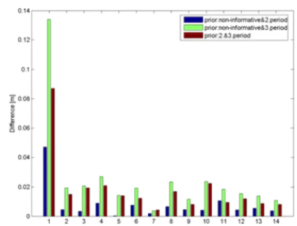
By using of non-informative information and the second period as a prior in the first period, the biggest difference is determined on point 1 with the value 4 cm. The smallest difference on point 5 with the value 0.03 cm is determined. For the same period, by using of non-informative informa-tion and the third period as a prior, the biggest difference is determined on point 1 with the value 13 cm. The smallest difference on point 7 is 0.4 cm. Finally, the biggest differ-ence is determined on point 1 with using the second period and the third period as priors, see Fig. 6a.
For the second period by using non-informative informa-tion and the first period as a prior we get the biggest dif-ference on point 1 with the value 4.72 cm and the smallest difference on point 5 with the value 0.14 cm. By using non-informative information and the third period as a prior, the biggest difference is determined on point 1 with the value 8.73 cm and the smallest difference on point 7 with the value 0.42 cm. For the same period, the first period and the third period are used as prior, the biggest difference is determined on point 1 with the value 13.42 cm and the smallest differ-ence on point 7 with the value 0.24 cm (see Fig. 6b). Almost the same procedures are done for the third period to evaluate Bayes Updating algorithm with different prior information. When we use non-informative information and the first pe-riod as a prior, we calculate the biggest difference on point 1 with the value 13.41 cm and the smallest difference on point 7 with the value 0.33 cm. In case of using non-informative information and the second period as a prior, the biggest dif-ference is determined on point 1 with the value 8.71 cm. The smallest difference can be found on point 7 with the value 0.50 cm. For the same period, first period and the second period were used as priors. This prior information let the biggest difference be on point 1 with the value 4.74 cm and the smallest difference on point 5 with the value 0.08 cm (see Table 4 and Fig. 6c).
3.5 Test of hypotheses for differences between different settings of methods and deformation between the mea-surement periods
In this section we compare the results obtained by differ-ent statistical methods described in previous sections. The
(a) BU by different prior information in the first period
(b) BU by different prior information in the second period
(c) BU by different prior information in the third period
. Differences between BU algorithms
Fig. 6. Differences between BU algorithms.
main question we discuss is whether the method chosen ma-jor influence on the outcome or not. The different methods are examined pairwise on equal estimations of parameters. Therefore we apply a multivariate test for equal mean vectors of parameter estimations. Again, we examine this hypothe-sis testing problem from a Bayesian viewpoint. The prior
Table 4. VR values for differences between different setting of BU algorithms (cm).
BU differences for 1. period
Prior period Prior period Prior period
non- informative 2. period non- informative 3. period 1. period 3. period
0.0935 0.2103 0.1495
BU differences for 2. period
non- informative 1. period non- informative 3. period 1. period 3. period
0.0902 0.1494 0.2094
BU differences for 3. period
non- informative 1. period non-informative 2. period 1. period 2. period
0.2138 0.1551 0.0855
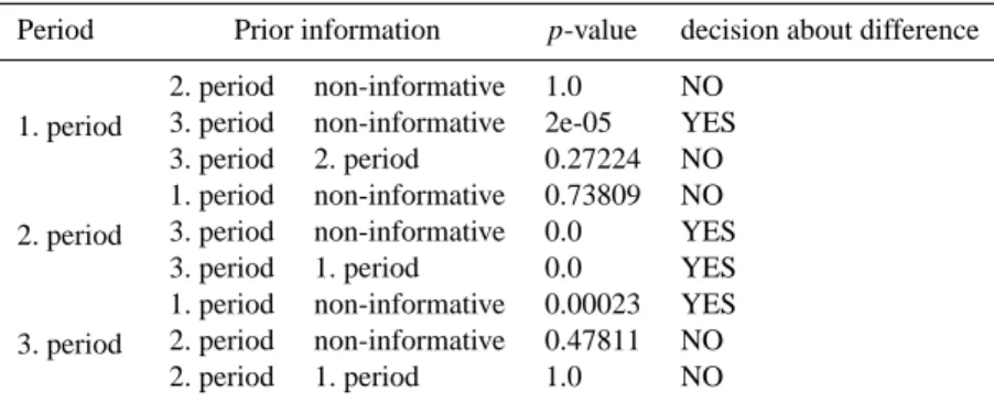
Table 5. p-values for differences between different settings of BU algorithms.
Period Prior information p-value decision about difference
1. period
2. period non-informative 1.0 NO 3. period non-informative 2e-05 YES 3. period 2. period 0.27224 NO 2. period
1. period non-informative 0.73809 NO 3. period non-informative 0.0 YES
3. period 1. period 0.0 YES
3. period
1. period non-informative 0.00023 YES 2. period non-informative 0.47811 NO
2. period 1. period 1.0 NO
distribution used is a Normal-Whishart distributions intro-duced as conjugate prior for the network structure in Sect. 1. The prior information is established in the same way as in the case of parameter estimation. Starting with vague prior the data of period 1, period 2 or period 3 are used as learning samples in turn.
Vague priors might be included in the range of conjugate priors in the sense that the vague prior is found as a limit of proper conjugate priors. Using vague priors for the param-eters, we find that the Bayesian testing statistics approaches classical testing statistics. The basis of the Bayesian decision
BF gives the Bayes-factor as follows
BF =
m(D|H0)
m(D|H1)
(17)
From a Bayesian context, the Bayes factor represents the testing statistics, that is the ratio of the marginal likelihoods on the assumption of the null-hypothesis and alternative hy-pothesis respectively. The marginals follow Eq. (5), note that in case of the alternative hypothesis the dimension of the multivariate Normal distribution differs from the case of
null-hypothesis. Methodological details of Bayesian testing in a multivariate model are explained in Rowe (2002).
Actually, the Bayes factor shows the results of tests. Any-way, Tables 5, 6 and 7 show p-values representing the result as well as for classical tests. Classical p-value, defined from a point null hypothesis, can be generalized in various ways. The p-value will be understood as a posterior p-value. That is the probability, given the data, that a future observation is more extreme (as measured by some test variable) than the data. Since we assessed vague priors in most cases our p-value makes little difference to the classical p-p-value.
In order to decide whether we have significant defor-mation or not between the measurement periods (e.g., be-tween period 1- period 2 or bebe-tween period 2- period 3), the p-values are calculated on the assumption of the null-hypothesis which accept there is no deformation between measurement period and alternative hypothesis which con-tradict with the null-hypothesis. The corresponding p-values for deformation analysis and decision about the deformation are given in Tables 8 and 9.
Table 6. p-values for difference between different settings of GS algorithms.
Period starting point p-value decision about difference
1. period 1 3 1.00000 NO 1 4 1.00000 NO 1 13 1.00000 NO 3 13 1.00000 NO 4 3 1.00000 NO 4 13 1.00000 NO 2. period 1 3 1.00000 NO 1 4 0.00002 YES 1 13 1.00000 NO 3 13 1.00000 NO 4 3 0.00015 YES 4 13 0.00015 YES 3. period 1 3 1.00000 NO 1 4 0.00000 YES 1 13 1.00000 NO 3 13 1.00000 NO 4 3 0.00000 YES 4 13 0.00000 YES
Table 7. p-values for difference between different settings of BU and GS algorithms.
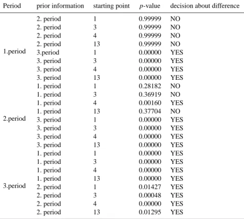
Period prior information starting point p-value decision about difference
1.period 2. period 1 0.99999 NO 2. period 3 0.99999 NO 2. period 4 0.99999 NO 2. period 13 0.99999 NO 3.period 1 0.00000 YES 3. period 3 0.00000 YES 3. period 4 0.00000 YES 3. period 13 0.00000 YES 2.period 1. period 1 0.28182 NO 1. period 3 0.36919 NO 1. period 4 0.00160 YES 1. period 13 0.37704 NO 3. period 1 0.00000 YES 3. period 3 0.00000 YES 3. period 4 0.00000 YES 3. period 13 0.00000 YES 3.period 1. period 1 0.00000 YES 1. period 3 0.00000 YES 1. period 4 0.00000 YES 1. period 13 0.00000 YES 2. period 1 0.01427 YES 2. period 3 0.00048 YES 2. period 4 0.00000 YES 2. period 13 0.01295 YES
Table 8. p-values calculated with the results from Bayes-Uptading for deformation analysis.
Method measurement periods subject prior information used p-values decision for deformation of the deformation in BU for each period
Bayes-Updating (BU)
1. period–2. period non-informative 0.00072 YES
1. period–2. period 3. period 0.99785 NO
2. period–3. period non-informative 0.00000 YES
2. period–3. period 1. period 0.00016 YES
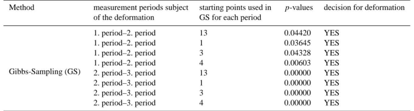
Table 9. p-values calculated with the results from Gibbs-Sampling for deformation analysis.
Method measurement periods subject starting points used in p-values decision for deformation of the deformation GS for each period
Gibbs-Sampling (GS)
1. period–2. period 13 0.04420 YES
1. period–2. period 1 0.03645 YES
1. period–2. period 3 0.04328 YES
1. period–2. period 4 0.00603 YES
2. period–3. period 13 0.00000 YES
2. period–3. period 1 0.00000 YES
2. period–3. period 3 0.00000 YES
2. period–3. period 4 0.00000 YES
4 Conclusions
In this paper we introduced two estimation procedures “Bayes-Updating” and “Gibbs-Sampling” based on Bayes theory for deformation monitoring networks which allows accounting for prior information about the coordinate param-eters. Gibbs-Sampling applies the simulation for the condi-tional distributions of parameter estimation of deformation network points. In Bayes-Updating algorithm, we can an-alyze the sensitivity of the model concerning the prior in-formation coming from different epoch measurements in de-formation network. In order to justify that the prior infor-mation is worth to consider, the significance test is applied on the Bayes-Updating results which varies according to dif-ferent prior information. Concerning usage of these two al-gorithms, Gibbs-Sampling algorithm takes more time com-pared to Bayes-Updating because simulation algorithm of Gibbs-Sampling depends on the information about the qual-ity of starting points itself. In this study we use a network with 14 points, when the user increase the number of net-work points, Gibbs-Sampling becomes complicated for such networks.
Comparing the results of the two parameter estimation procedures we get differences of network point coordinates on cm level. When we consider all these parameter estima-tion results as input data for deformaestima-tion analysis, it should be pointed out here that the estimation procedure which is used in individual epochs has also big importance as defor-mation analysis procedures itself.
The results of significance test for difference between dif-ferent setting of GS algorithm show that the estimate is sensi-tive to the choice of starting point, for example starting point 4 leads to difference in the results, see Table 6. The differ-ences for BU algorithms indicate that third period as a prior information leads to differences on the results more than the other periods, see Table 5 for significance test and Table 4 for variances. From the comparison between BU and GS algorithms, we conclude that third period as a prior informa-tion in BU algorithm and starting point 4 in GS algorithm leads significance of difference on the results. It should be mentioned here third period as a data in BU leads to signif-icance of difference w.r.t. any prior information, see Table 7 for significance test and Table 3 for variance. The hypothesis test for deformation out of BU results exhibits significance of difference between first period-second period and second period-third period except in case of using third period as a prior information, see Table 8. Therefore, we can conclude from this study that the prior information has impact on the results of BU algorithm. The same hypothesis test out of GS results indicates also deformation with evident deformation effect between second period-third period and less significant testing results by p-values near to the critical value 0.05, see Table 9. The season which our 2. period (February) and 3.pe-riod (May) measurements corresponded to is a danger season with spring rainfall and snow melting in East Black Sea Re-gion for landslides. The significance deformation which we got out of our testing for 2. period and 3.period might be a result of this.
Acknowledgements. This study was done during the first author’s
research stay at the Institute of Statistics and Probability Theory at Vienna University of Technology (TU Vienna) and financially supported by Natural Science Institute of Karadeniz Technical University and TU Vienna. The first author is thankful to R. Viertl, head of the Statistics and Probability Theory Institute in TU Vienna, for providing her full scientific facilities during her research stay at this institute.
Edited by: Kang-tsung Chang
Reviewed by: three anonymous referees
References
Albertella, A., Cazzaniga, N., Sans`o, F., Sacerdote, F., Crespi, M., and Luzietti, L.: Deformations detection by a Bayesian ap-proach: prior information representation and testing criteria def-inition, ISGDM2005 – IAG Symposium volume n. 131, 2005. Caspary, W. F.: Concept of network and deformation analysis,
Monograph 11, School of Geomatics Engineering, The Univer-sity of New South Wales, Australia, 2000.
Felsenstein, K.: Mathematische methoden f¨ur die interpretation von risiken, Imago Hominis, 11, 261–269, 2004.
Felsenstein, K.: Bayesian interpolation schemes for monitoring sys-tems. In: Advances in model-oriented design and analysis, 6, Physica-Verlag, Heidelberg, 2001.
Felsenstein, K.: Bayes’sche statistik f¨ur kontrollierte experimente, Vandenhoeck and Ruprecht, G¨ottingen, 1996.
Koch, K. R.: Bayesian Inference with Geodetic Applications, Springer, Berlin, Heidelberg, New York, 1990.
Ocakoglu, F., Gkceoglu, C., and Ercanoglu, M.: Dynamics of a Complex Mass Movements Triggered by Heavy Rainfall: A Case Study from NW Turkey, Geomorphology, 42, 329–341, 2002. ¨
Onalp, A.: Landslides of East Black Sea Region – Reasons, Analy-sis and Controls, 1st National Landslides Symposium of Turkey, Trabzon, Proceedings Paper, 85–95, (in Turkish), 1991. Robert, C. and Casella, G.: Monte Carlo statistical methods
Springer, New York, 2004.
Robert, C.: The Bayesian Choice, Springer, New York, 2001. Roberts, G. and Rosenthal, J.: Markov chain Monte Carlo: Some
practical implications of theoretical results, Canadian J. Statist., 25, 5–32, 1998.
Rowe, D.B.: Multivariate Bayesian Statistics, Chapman and Hall/CRC, London, 2002.
Tarhan, F.: A look to landslides of East Black Sea Region, 1st Na-tional Landslides Symposium of Turkey, Trabzon, Proceedings Paper, 38–63 (in Turkish), 1991.
Yalcinkaya, M. and Bayrak, T.: Dynamic model for monitor-ing landslides with emphasis on underground water in Trabzon province, Northeastern Turkey, Journal of Surveying Engineer-ing, August 2003, 129(3), 115–124. 2003.
Yalcinkaya M., Tanir, E.: A study on using Bayesian statis-tics in geodetic deformation analysis, Proceedings 11th Interna-tional FIG Symposium on Deformation Measurements, Santorini (Thera) Island, Greece, 25–28 May 2003, 2003.
Yalcinkaya, M. and Bayrak, T.: Comparison of static, kinematic and dynamic geodetic deformation models for Kutlug¨un landslide in northeastern Turkey, Natural Hazards, January 2005, 34(1), 91– 110, 2005.