HAL Id: insu-01564674
https://hal-insu.archives-ouvertes.fr/insu-01564674
Submitted on 13 Jan 2021
HAL is a multi-disciplinary open access
archive for the deposit and dissemination of
sci-entific research documents, whether they are
pub-lished or not. The documents may come from
teaching and research institutions in France or
abroad, or from public or private research centers.
L’archive ouverte pluridisciplinaire HAL, est
destinée au dépôt et à la diffusion de documents
scientifiques de niveau recherche, publiés ou non,
émanant des établissements d’enseignement et de
recherche français ou étrangers, des laboratoires
publics ou privés.
Emmanuel Marcq, Arnaud Salvador, Hélène Massol, Anne Davaille
To cite this version:
Emmanuel Marcq, Arnaud Salvador, Hélène Massol, Anne Davaille. Thermal radiation of magma
ocean planets using a 1-D radiative-convective model of H2O-CO2 atmospheres. Journal of
Geo-physical Research. Planets, Wiley-Blackwell, 2017, 122 (7), pp.1539-1553. �10.1002/2016JE005224�.
�insu-01564674�
Thermal radiation of magma ocean planets using a 1-D
radiative-convective model of H
2
O-CO
2
atmospheres
E. Marcq1 , A. Salvador2,3, H. Massol3, and A. Davaille2
1LATMOS/IPSL, Université Paris-Saclay, Guyancourt, France,2FAST, CNRS/Université Paris Sud, Université Paris-Saclay,
Orsay, France,3GEOPS, Université Paris-Saclay, Orsay, France
Abstract
This paper presents an updated version of the simple 1-D radiative-convective H2O-CO2 atmospheric model from Marcq (2012) and used by Lebrun et al. (2013) in their coupled interior-atmosphere model. This updated version includes a correction of a major miscalculation of the outgoing longwave radiation (OLR) and extends the validity of the model (P coordinate system, possible inclusion of N2, and improved numerical stability). It confirms the qualitative findings of Marcq (2012), namely, (1) the existence of a blanketing effect in any H2O-dominated atmosphere: the outgoing longwave radiation (OLR) reaches an asymptotic value, also known as Nakajima’s limit and first evidenced by Nakajima et al. (1992), around 280 W/m2neglecting clouds, significantly higher than our former estimate from Marcq (2012). (2) The blanketing effect breaks down for a given threshold temperature T𝜀, with a fast increase of OLR with increasing surface temperature beyond this threshold, making extrasolar planets in such an early stage of their evolution easily detectable near 4 μm provided they orbit a red dwarf. T𝜀increases strongly with H2O surface pressure, but increasing CO2pressure leads to a slight decrease of T𝜀. (3) Clouds act bothby lowering Nakajima’s limit by up to 40% and by extending the blanketing effect, raising the threshold temperature T𝜀by about 10%.
Plain Language Summary
Recently formed Earth-sized planets experience a “magma ocean” stage, where molten rocks extend from the core up to the surface. These planets are able to cool themselves by radiating more heat through their thick atmospheres than they absorb from their parent star. We have investigated the effect of the total atmospheric content (assumed to consist mostly of water vapor and carbon dioxide) and of the surface temperature of the magma ocean upon the rapidity of the cooling. Our main finding is that there are two stages: for very high surface temperatures, cooling is fast, and only thin clouds can form. Such planets would be quite easily detected since they radiate very efficiently in the infrared range. Conversely, relatively cool surface temperatures lead to cooler upper atmospheres, harboring thick water clouds. Such planets would be very difficult to distinguish from more mature planets such as Earth or Venus from the point of view of a remote observer.1. Introduction
Young telluric planets are expected to harbor very different atmospheres compared to those we already know about. Even restricting the field of study to only secondary atmospheres—so after the lightest elements (He and H2) have escaped—the 107years or more required to significantly alter the composition of C−, N−, or O− bearing volatiles through atmospheric escape may result in much heavier atmospheres than even present-day Venus. Another specificity of such young planets is that their internal heat flux is several orders of magnitude larger than more mature planets like present-day Earth, for example, and can be comparable to the stellar fluxes while in their magma ocean stage; this pushes these atmospheres out of global radiative balance, mak-ing them radiate significantly more energy to outer space than they absorb from their host stars. Since most atmospheric models assume a negligible geothermal heat flux, they cannot be used here. Furthermore, since the interaction between these early atmospheres with both the interior and escape processes is significant, specific coupled models are required to proceed.
However, very dense telluric atmospheres are also expected in other situations, namely, when modeling run-away atmospheres: these atmospheres usually include a full Earth ocean equivalent (300 bar) as atmospheric water vapor. It is therefore of no surprise that some of the earlier models partially relevant for our studies deal
RESEARCH ARTICLE
10.1002/2016JE005224
Key Points:
• Thermal blanketing confirmed at almost equal to 280 W/m2, for steam-dominated atmospheres (Nakajima’s limit) around magma ocean planets
• Thermal blanketing effective only for surface temperatures lower than a threshold, depending mainly upon the atmospheric water content • Detectability prospects for hot extrasolar magma ocean planets orbiting red dwarfs are optimal (contrast over 10%) near 4 micrometer
Correspondence to:
E. Marcq,
Citation:
Marcq, E., A. Salvador, H. Massol, and A. Davaille (2017), Thermal radiation of magma ocean planets using a 1-D radiative-convective model of H2O-CO2atmospheres, J.
Geophys. Res. Planets, 122, 1539–1553,
doi:10.1002/2016JE005224.
Received 28 NOV 2016 Accepted 22 JUN 2017
Accepted article online 27 JUN 2017 Published online 26 JUL 2017
©2017. American Geophysical Union. All Rights Reserved.
with such atmospheres [Komabayashi, 1967; Ingersoll, 1969; Kasting, 1988; Nakajima et al., 1992]. In the context of exoplanetary studies, investigating the inner, runaway-limited edge of the habitability zone has received a lot of recent attention using general circulation models or simple 1-D columns [Leconte et al., 2013; Goldblatt
et al., 2013; Kopparapu et al., 2013; Yang et al., 2014; Yang and Abbot, 2014; Hamano et al., 2015; Kopparapu et al., 2016].
Recently outgassed atmospheres around magma ocean planets and out of global radiative balance were first numerically investigated in the 1980s [Abe and Matsui, 1988]. Such models are still being developed nowadays [Elkins-Tanton, 2008; Marcq, 2012; Lebrun et al., 2013; Hamano et al., 2013, 2015; Lupu et al., 2014; Schaefer et al., 2016], with various levels of complexity or coupling. We aim to present here the most recent updates to the 1-D radiative-convective model of Marcq [2012] used by Lebrun et al. [2013] and Salvador et al. [2017]. We will first detail our improvements in section 2. In section 3, we will review our updated results, and how they bear on the detectability of magma ocean planets. Finally, we will conclude and discuss the limitations of our model in section 4.
2. Model Description
2.1. Thermal Structure
As in Marcq [2012], up to three different physical layers (not to be confused with the computational layers, which are typically a few hundred) are possible in this model. From the bottom up (as can be seen in Figures 7 and 9), they are, namely, the following: (1) unsaturated troposphere, (2) moist troposphere, and (3) meso-sphere. Moist troposphere is present only if the saturation of water vapor is reached at any altitude—if this occurs at the surface, then unsaturated troposphere will not exist, and any water in excess of 100% saturation is assumed to condense and form a water ocean overlying the magma ocean.
2.1.1. Unsaturated Troposphere
This lowermost convective layer follows, as in Marcq [2012], a dry adiabatic lapse rate. In terms of the new pressure coordinate, (𝜕T∕𝜕P)Sfollows Kasting [1988]:
(𝜕T∕𝜕P)S= [ 𝜌vT ( 𝜕Vv∕𝜕T ) P ] ∕[𝜌vCP,v(T) +𝜌cCP,c(T) +𝜌oCP,o(T)], (1) where Vv= 1∕𝜌vis the specific volume of water vapor.
The thermodynamical properties of water vapor are computed using the Fortan NBS/NRC steam tables [Haar
et al., 1984], which implies that H2O is not considered as an ideal gas in our model—this is required since the critical point of water lies within the range of modeled pressures and temperatures. CO2and N2, on the other hand, are always considered as ideal gases since the (T, P) range of our model lies very far from their critical points. CP,c(T) for CO2follows the expression from Abe and Matsui [1988]. CP,o(T) is approximated by the analytic expression CP,o(T) = 1040 + 488(e−688.1 K∕T)2in J/kg/K, fitted in the 300 to 2500 K temperature range from Chase [1998] National Institute of Standards and Technology data.
2.1.2. Moist Troposphere
This layer is still convective, but H2O condensation takes place so that the lapse rate is now given by the following: (𝜕T∕𝜕P)S=[(dPsat∕dT ) +𝜌nR∕Mn ( 1 +𝜕 ln 𝜌v∕𝜕 ln T − 𝜕 ln 𝛼v∕𝜕 ln T )]−1 (2) Here𝜌n=𝜌c+𝜌o, and Mnstands for the weighted molecular mass of the non condensible CO2-N2mixture. Following Kasting [1988], we define𝛼v=𝜌v∕𝜌n, and its derivative𝜕 ln 𝛼v∕𝜕 ln T is computed according to the formula given in Marcq [2012] and Kasting [1988]:
𝜕 ln 𝛼v∕𝜕 ln T = R∕Mn ( 𝜕 ln 𝜌v∕𝜕 ln T ) − Cv,n(T) −𝛼v(𝜕sv∕𝜕 ln T) 𝛼v ( sv− sc ) + R∕Mn (3)
with scstanding for the specific entropy of condensed water.
Wordsworth and Pierrehumbert [2013] recently showed that the above expression is only valid when both
water vapor and the CO2-N2mixture can be considered as ideal gases. Although, strictly speaking, this is not the case in our model regarding H2O, water condensation usually occurs at higher altitudes, and therefore
relatively low pressure and temperature, far from the critical point of water. Departure between our H2O ther-modynamical tables and ideal gas was empirically found to be less than a few percents in these layers, so that we could still make use of the derivation from Kasting [1988] in most situations.
2.1.3. Mesosphere
Since our model does not include yet any radiative transfer for the incoming short wave stellar radiation, we are unable to reproduce any stratosphere (defined as a radiative, nonconvective layer where temperature increases with increasing height). Therefore, we call mesosphere the radiative, nonconvective layer on top of the troposphere. The base of our mesosphere (the tropopause) is reached once the tropospheric temperature falls below a given temperature T0. Although the local radiative equilibrium would allow an iterative calcula-tion of the mesospheric temperature profile, its integrated Rosseland opacity was empirically found to be thin. Our simple model therefore considers this mesosphere as an isothermal layer at the temperature T0, and thus
dT∕dP = 0 there.𝛼vis also considered vertically uniform in this layer. However, it is noteworthy that real gas effects may lead to strong departures from this prescribed isothermal profile, but a more realistic computation of the radiative temperature profile would require the inclusion of stellar radiation.
T0can therefore be understood as the top of atmosphere (TOA) temperature of our model. Kasting [1988] sets it to 200 K, but our model is intended to apply to even hotter atmospheres. There are two options for the final user here: (1) fix T0to a constant temperature; standard choices are 200 K for an H2O-rich mesosphere as Kasting [1988] did, or even colder as long as CO2is a major constituent. For example, TOA temperature is close to 150 K for [Leconte et al., 2013], and this cold TOA temperature issue is also extensively discussed by
Wordsworth and Pierrehumbert [2013]—let us also mention that at the very top of our model, NLTE (nonlocal
thermodynamical equilibrium) effects could kick in for CO2radiative cooling so that even the most precise line-by-line LTE calculations would not be accurate. The second option (2) is to adjust iteratively T0so that the relative divergence of outgoing longwave radiation (OLR) at the top of our model (P = 0.1 Pa, 𝜏i∼ 0):
|| || |
∑
i∈bandskabs,i𝜕OLRi∕𝜕𝜏i
∑
i∈bandskabs,iOLRi
|| ||
|< 0.02 (4) This adjustment results in very cold mesosphere (T0around 150 K or less) even when the surface temperature is very hot. Since Kasting [1988] found that total OLR was not much dependent on his prescribed value T0as long as T0< 240 K—cool mesospheres do not contribute much to the thermal radiation. Therefore, since we do not include yet any radiative stellar heating of these layers (that could dramatically rise their temperature) and following similar temperature profiles from Lupu et al. [2014], we hereafter adopt a fixed value T0= 200 K.
2.2. Radiative Calculations 2.2.1. Short Wave Radiation
Shortwave radiation is not taken into account in this model, as in Marcq [2012]. Its effect on the radiative budget of the planet is parameterized through a bolometric albedo A, so that the absorbed stellar radiation is computed as (1 − A)F∗where F∗is the integrated stellar constant. In this version of the model, A is computed as A = Aclear(1 − e−𝜏c) + Acloude−𝜏cwhere𝜏cstands for the optical depth of the clouds (when present and
considered) in the visible range—this enables a smooth transition when clouds appear and thus avoids any threshold effect. Since the temperature profile is not computed from the radiative fluxes (except optionally for T0, see section 2.1.3), this crude parameterization is valid to estimate the radiative balance of the planet. Please note that this albedo parameterization is only used in coupled interior-atmosphere simulations and is irrelevant when discussing the sole atmospheric subsystem, as is the case in this paper.
The former version of the model used different values for Aclear= 0.2 (Mars like) and Aclouds= 0.7 (Venus like); however, recent progress in dense atmosphere radiative transfer modeling [Leconte et al., 2013; Hamano et al., 2015; Kopparapu et al., 2013; Goldblatt et al., 2013] showed that the albedo of H2O-rich atmospheres is always quite low, even when thick clouds are present. Therefore, following Leconte et al. [2013] who unlike other stud-ies took into account the radiative effect of clouds, the coupled simulations of Salvador et al. [2017] primarily use Aclear= Acloud= 0.2, although the final user can still choose different values for Aclearand Acloud. The albedo could however be substantially higher (equal or above 0.5) for CO2-rich, H2O-poor atmospheres [Kopparapu
et al., 2013, their Figure 5] or for slow rotating planets exhibiting permanent convective clouds near the
sub-stellar point [Yang et al., 2013]. This further highlights the need for an improved short wave radiation scheme in a future version of our model (see section 4.1.2).
2.2.2. Long Wave Radiation
In our model, the thermal radiation encompasses wave numbers between 0 and 10,100 cm−1. This ther-mal radiation can be computed either (1) following the gray approximation in the aforementioned range or (2) using a k correlated radiative transfer code. The former yields cruder estimates of the resulting OLR, but is much faster, and can therefore be used in first, exploratory simulations where no spectroscopic out-put is needed. We use the discrete ordinates radiative transfer (DISORT) [Stamnes et al., 1988] solver with four streams in the whole atmosphere, so that scattering (e.g., by clouds, see after) can be taken into account. We now discuss the sources of long wave opacity provided as inputs to DISORT.
In the gray approximation, the mass absorption coefficients of H2O and CO2are, respectively, set equal to 10−2and 10−4m2/kg following Nakajima et al. [1992]. Our k-correlated code uses the same high-resolution spectrum (truncated at 100 cm−1to avoid any overlap with continuum opacity, see below) computed by KSPECTRUM [Eymet et al., 2016] as Leconte et al. [2013] and also shares the same choice of 16 g values. The set of corresponding 16 k coefficients is then stored in a three-dimensional look-up table (H2O/CO2ratio, temperature, and total pressure including N2) suitable for fast interpolation. This extensive rewriting of the
k-correlated code led us to correct a major mistake in the first published version of Marcq [2012] that resulted in a severe underestimation of the resulting OLR by a factor of about 2. Therefore, the atmosphere and the coupled magma ocean should be cooling faster than previously reported by Lebrun et al. [2013]. This will be further discussed in section 3.4.
Continuum opacity is calculated and added in both gray and k-correlated cases and is unchanged since Marcq [2012]: H2O-H2O continuum opacity is taken from Clough et al. [2005], and CO2-CO2fitted from Venus obser-vations by Bruno Bézard [Bézard et al., 2011; Marcq et al., 2008]. H2O-CO2continuum opacity is not considered, and in any case negligible compared to H2O-H2O [Ma and Tipping, 1992, their Figure 7] and/or CO2-CO2 depending on the dominant species in the atmosphere.
2.2.3. Clouds
Clouds are considered present throughout the atmosphere wherever H2O saturation occurs, i.e., in the moist tropospheric layer. Their radiative effect is taken into account through albedo parameterization for the stel-lar radiation (see section 2.2.1), and in the radiative transfer code for the thermal radiation. Their optical properties and microphysical properties—mass loading,𝜛0(𝜆), g(𝜆), Henyey-Greenstein phase function, and
Qext(𝜆)—still follow the simple parameterization from Kasting [1988] and already used in Marcq [2012]. How-ever, since a realistic modeling of the radiative budget of clouds is not possible in a 1-D atmospheric column model such as ours, the user can choose to disable the scattering of thermal radiation by these clouds. Also, we do not couple our atmospheric model to a microphysical model, so that our cloud layer parameterization probably overestimates their actual thickness—as an example, when running with present-day Earth setup, our model finds thick clouds extending in the whole troposphere, from the surface up to 10 km, with an opti-cal thickness close to 300 at 1 μm. So one can compute OLR with and without taking into account the radiative effects of the cloud cover, knowing that the actual OLR is bracketed between these two extreme situations. Also, it is worth noting that scattering and/or absorbing mesospheric photochemical aerosols (not included in our model) could lead to a further decrease in OLR as well as alter the temperature profile.
3. Results
3.1. OLR Versus Tsurf
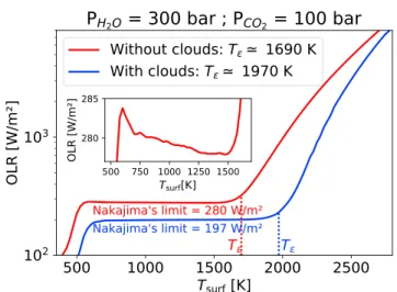
In most situations, water vapor is present in sufficient quantity (i.e., Psurf(H2O)>[Psurf(CO2)∕15bar]1.6× 1 bar according to Figure 5; see section 3.1.2 for further discussion) in the atmosphere. In such a case, the variation of spectrally integrated OLR with respect to the surface temperature displays the features visible in Figure 1. These common features are (#1) the existence of an asymptotic regime at relatively low temperatures, where the OLR is quite low (the so-called blanketing effect) and exhibits very little dependency with surface temper-ature; (#2) at higher surface temperatures, the OLR increases rapidly with surface tempertemper-ature; (#3) optically thick clouds have two main effects: (#3a) they substantially lower the asymptotic OLR, and (#3b) they extend the blanketing effect to higher surface temperatures—at very high surface temperatures, clouds become optically thinner and thinner; thus, both scenarios yield the same OLR.
Features #1 and #2 have been consistently reproduced by all similar radiative-convective models used for both models of atmospheres around magma ocean planets [Hamano et al., 2013; Marcq, 2012] or, more often, studying the runaway greenhouse effect [Kasting, 1988; Nakajima et al., 1992; Goldblatt et al., 2013]. In fact,
Figure 1. Outgoing longwave radiation (OLR) versus surface temperature for a total volatile inventoryPsurf(H2O) = 300bar andPsurf(CO2) = 100bar neglecting (red) or taking into account (blue) the radiative effect of water clouds extending throughout the moist troposphere. The small decrease in OLR forTsurf< T𝜀is shown in insert.
the very existence of this near-asymptotic behavior of OLR versus Tsurfis responsible for the instability char-acterizing the runaway greenhouse effect: a tiny increase in absorbed solar radiation (and also of equal OLR when in global radiative balance) can trigger a rise of surface temperature by several hundreds of kelvins until global radiative balance is restored at a very high surface temperature. Actually, OLR decreases by a few W/m2with increasing surface temperatures below 1400 K for such atmospheres, as shown in the insert from Figure 1. This counterintuitive effect arises in H2O-CO2radiative-convective models as explained by Nakajima
et al. [1992]: thermal brightness for a given wavelength is directly related to vertically integrated lapse rate dT∕d𝜏 above 𝜏 = 1, which usually lies within the moist troposphere. A hotter surface temperature will
there-fore move the moist troposphere upward to lower pressure levels, thus lowering the moist lapse rate. This OLR decrease results in an even more unstable situation as a straight plateau and can be a source of hysteresis in the context of interior-atmospheres models where coupling is performed using the internal heat flux [e.g.,
Salvador et al., 2017]: two very different surface temperatures yield the same OLR and therefore require the
same internal heat flux.
In the context of magma ocean planets, such an efficient blanketing effect can be reached only for planets far enough from their host star (so-called Hamano-type I planets) and thus able to reach global radiative balance below this asymptotic value. This value is also known as Nakajima’s limit (NL) since it was accurately described for the first time by Nakajima et al. [1992]. Further study of NL in our model and comparison with other works is found in section 3.1.2.
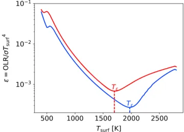
We can define formally the aforementioned blanketing effect through an effective emissivity𝜀 defined as OLR = 𝜎Teff4 = 𝜀𝜎T
surf4—the smaller the value of𝜀, the stronger the blanketing effect. It appears (see Figure 2) that𝜀 exhibits a minimum with respect to Tsurffor a given value Tsurf = T𝜀. Thus, T𝜀provides a self-consistent and physically sound threshold to distinguish the low-temperature regime Tsurf < T𝜀from
the high-temperature regime Tsurf> T𝜀, even for CO2-rich atmospheres which do not exhibit the asymptotic regime at OLR = NL for Tsurf < T𝜀(see Figure 3). The variations of T𝜀with respect to H2O and CO2surface pressures will be addressed in section 3.1.1.
Features #3a and #3b are not reproduced by all models, and heavily dependent on the assumptions regard-ing the physical properties of the cloud layers. Kastregard-ing [1988] already performed a sensitivity study on the radiative effect of cloud layers depending on their vertical location and found their influence from moderate (decreasing OLR by a few tens of percents) to negligible. As previously discussed, our parameterization (clouds extending throughout the whole moist troposphere) yields the optically thickest scenario. Others have faced these problems before [Hamano et al., 2015; Kopparapu et al., 2013], and it appears that no satisfactory repre-sentation of clouds can be performed using a 1-D column model like ours—this is mainly due to the nonlinear radiative effects of clouds upon the OLR. Also, due the complexity of the involved microphysics, even 3-D models are unlikely to yield a satisfactory representation of the clouds in the near future.
Figure 2. Graphical determination ofT𝜀from𝜀 = f(Tsurf)for both OLR plotted in Figure 1.
3.1.1. T𝜺Versus Atmospheric Inventory
Figure 4 shows the behavior of threshold temperature T𝜀as defined in the previous section. As expected, the efficiency of the blanketing effect at higher surface temperatures is dominated by the total water vapor atmospheric content. This reflects the well-known fact that H2O is a much more efficient greenhouse gas than CO2.
Aside from the low H2O-high CO2situation—which does not actually exhibit asymptotic limit for Tsurf< T𝜀,
see section 3.1.2—we can see that with a fixed atmospheric water vapor content, adding more CO2in the atmosphere is actually detrimental to the blanketing effect. This may come as a surprise but can be under-stood as follows. As previously stated here and following Nakajima et al. [1992], the thermal brightness for a given wavelength is related to the vertically integrated lapse rate dT∕d𝜏 above the 𝜏 ∼ 1 level, which for most wavelengths is located in the higher troposphere. Adding more CO2while keeping H2O the same results in a lower humidity ratio𝛼vin the troposphere, which in turn leads to a steeper adiabatic lapse rate (in terms of
dT∕d𝜏, since CO2mass absorption coefficient is much lower than for H2O). This results in an increase of OLR for a given surface temperature, thus weakening the blanketing effect.
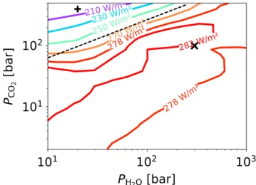
The variations of T𝜀for a large domain in 10 bar< Psurf(H2O) < 300 bar and 5bar < Psurf(CO2) < 100 bar according to Figure 4 are approximated by ΔT𝜀∕T𝜀≈ 0.22ΔPsurf(H2O)∕Psurf(H2O)−0.05ΔPsurf(CO2)∕Psurf(CO2), which yields after integration an approximate analytical parameterization:
T𝜀≈ 1420K [P surf(H2O) 100bar ]0.22[P surf(CO2) 30bar ]−0.05 (5)
Figure 4. Contour plot of threshold temperatureT𝜀versus surface pressuresPsurf(H2O)andPsurf(CO2). Cross sign indicates the atmospheric inventory from Figure 1, and plus sign the atmospheric inventory from Figure 6. Dashed lines indicate the approximate analytical parameterization stated in section 3.1.1.
3.1.2. Nakajima’s Limit Versus Atmospheric Inventory
Figure 5 shows the asymptotic Nakajima’s limit, estimated here using OLR (Tsurf = 800 K) since 800K < T𝜀 in the investigated (PH
2O, PCO2) parameter space. Its most striking feature is a sharp boundary (shown as
a dashed line in Figure 5 between the CO2-dominated atmospheres in the upper left corner (Psurf(H2O)> [
Psurf(CO2)∕15bar ]1.6
× 1 bar, and H2O-dominated atmospheres (everywhere else).
For H2O-dominated atmospheres, NL is remarkably independent of the exact atmospheric composition and/or surface pressure, with values ranging between 275 and 283 W/m2, well above Marcq [2012] uncor-rected estimate of 220 W/m2. This corrected value is in a very good agreement (within 2.5%) with recent runaway greenhouse studies, whether using a line-by-line [Goldblatt et al., 2013] (282 W/m2) or k-correlated [Leconte et al., 2013] (also 282 W/m2) radiative transfer code. This qualitative behavior was also reproduced by older random band or gray models [Nakajima et al., 1992; Kasting, 1988], albeit with larger values for NL on the order of 300 W/m2or more. A detailed physical interpretation about how all steam-dominated atmospheres exhibit this same NL value can be found in Goldblatt et al. [2013]: as long as the mesosphere is cool enough, the T(p) profile in the atmospheric layers that contribute to the OLR is mostly unchanged, although the alti-tude of these layers may vary greatly. The small variations of ±2 W/m2we find for NL originate probably from the fact that we estimate the asymptotic NL with a more computationally robust proxy OLR (Tsurf = 800 K):
Figure 5. Contour plot of OLR (Tsurf= 800K) (indicative of Nakajima’s limit value) versus surface pressuresPsurf(H2O) andPsurf(CO2). Cross sign indicates the atmospheric inventory from Figure 1, and plus sign the atmospheric inventory from Figure 6. A dashed line separates H2O-dominated atmospheres from CO2-dominated atmospheres.
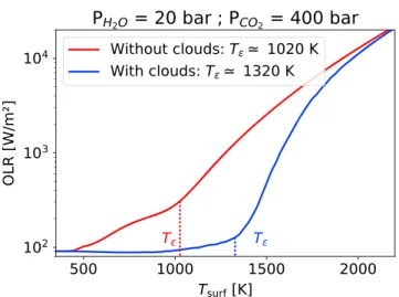
Figure 6. Outgoing longwave radiation (OLR) versus surface temperature for a total volatile inventoryPsurf(H2O) =
20bar andPsurf(CO2) = 400bar neglecting (red) or taking into account (blue) the radiative effect of water clouds extending throughout the moist troposphere.
there is indeed a local maximum for OLR = f (Tsurf) at relatively cool Tsurfvalues for H2O-CO2atmospheres as seen and discussed by Nakajima et al. [1992, their Figure 6], and the OLR at Tsurf= 800 K might be influenced by this maximum and shifted then to slightly higher values compared to the actual NL.
On the other hand, for CO2-dominated atmospheres, the OLR at Tsurf= 800 K is varying with the atmospheric composition and decreases strongly with increasing CO2content (see Figure 5). Further investigations show that for these atmospheres, the function OLR = f(Tsurf)does not exhibit any asymptotic behavior as can be seen in Figure 1 but rather increases monotonically with increasing Tsurfas can be seen in Figure 6—although effective emissivity𝜀 still displays a local minimum with respect to Tsurf, so that our definition of T𝜀remains
valid. Since CO2partial pressure, unlike H2O, is not governed by its saturated vapor pressure in radiatively active layers, the reasoning from Goldblatt et al. [2013] does not apply to these atmospheres, which accord-ingly cannot be said to be experiencing a runaway H2O greenhouse. It is therefore misleading to define a Nakajima’s limit for these atmospheres. One could remark that the present-day Venusian atmosphere, with an OLR near 170 W/m2for P
surf(CO2) = 92 bar and Psurf(H2O) ≈ 3 mbar, is fully representative of this CO2-dominated regime although we did not perform simulations with such a low water abundance. Let us finally note that a CO2-dominated atmosphere is not expected for a recently outgassed atmosphere prior to differential atmospheric escape, so that we will restrict the discussion in the next sections to more typical H2O-dominated atmospheres.
3.2. Vertical Structure and Low Resolution OLR Spectra 3.2.1. Tsurf< T𝜺
A typical atmospheric structure for H2O-dominated atmospheres in the Tsurf< T𝜀regime is shown in Figure 7.
The three-stage structure is well visible here, and in some way reminiscent of an exaggerated present-day Venus: from the bottom up, a clear unsaturated layer with no possible condensation, then a saturated layer where condensation may occur over several scale heights and form thick clouds, underneath a relatively cool (200 K) isothermal mesosphere. Such a structure is here again typical of runaway atmospheres, and extensively discussed by, e.g., Goldblatt et al. [2013]: altering Tsurfin this regime merely squeezes or expands the thickness of the lowermost unsaturated layer, while most of the thermal emission originating from overlying layers (in the uppermost moist troposphere and lower mesosphere) which are at more or less constant temperatures, hereby keep OLR constant with respect to the surface temperature at Nakajima’s limit.
The thermal spectra (with or without taking into account the radiative effect of clouds) originating from the same atmosphere are shown in Figure 8. This spectrum is remarkably independent of surface temperature for Tsurf < T𝜀, and very similar to other runaway atmospheres OLR spectra such as Hamano et al. [2015, their Figure 11] or Goldblatt et al. [2013, their Figure 1]. As could be expected, the spectral features of such atmo-spheres are dominated by water vapor, with some CO2absorption bands barely noticeable near 15 and 4.3 μm. From the spectroscopic analysis of their OLR, these atmospheres cannot be told apart from more evolved
Figure 7.T(z)profile in aTsurf= 1200K< T𝜀≈ 1690K forPsurf(H2O) = 300bar andPsurf(CO2) = 100bar.
planets at global radiative balance and hosting a thick H2O-CO2atmosphere, somewhat analogous to (a much wetter) Venus. This similarity even extends to featuring near infrared windows (of both H2O and CO2in this case) where the brightness temperature can exceed 400 K depending on the cloud cover. An extensive discus-sion on the detectability of such planets can be found in Hamano et al. [2015] for their type I planets, defined as the planets that are able to reach global radiative balance for such relatively low surface temperatures. We further quantitatively discuss the detectability of similar exoplanets in section 3.3.
3.2.2. Tsurf> T𝜺
A typical atmospheric structure in the Tsurf> T𝜀regime is shown in Figure 9. The vertical extension of the
saturated layer is much thinner in this case, and it is also located at much lower pressure levels so that the mass loading (and, therefore, the optical thickness) of the clouds is much lower.
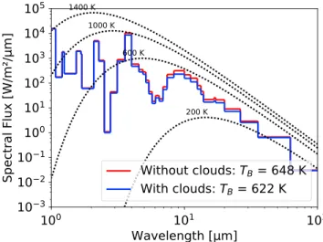
The very high tropopause in these cases results in having most of the thermal emission originating from the hotter, unsaturated troposphere. This enables the OLR to break Nakajima’s limit. For example, the spectrum associated with the atmospheric structure shown in Figure 9 is shown in Figure 10. Their brightness tempera-ture for𝜆 > 10μm is relatively low (equal to the mesospheric temperature), but most of their thermal emission actually comes from shorter wavelength and concentrated in the few near infrared windows of H2O and CO2, below 5μm. Also, the optically thin clouds would have little effect on the spectra in such atmospheres. Our cut-off for thermal IR calculations near 1 micron could be challenged here, since the spectrum shown in Figure 10
Figure 8. Thermal emission spectrum for the atmosphere shown in Figure 7. The blue spectrum takes into account the
radiative effect of clouds, whereas the red spectrum does not. Dotted lines stand for Planck functions at the indicated temperatures.
Figure 9.T(z)profile in aTsurf= 2800K> T𝜀≈ 1690K forPsurf(H2O) = 300bar andPsurf(CO2) = 100bar.
displays significant thermal emission near 1 micron and probably also for shorter wavelength, so that there might be a visible “thermal glow” for such atmospheres, as can be seen in the analogous spectrum of Hamano
et al. [2015, their Figure 1a]. However, the resulting underestimation of OLR is found to be small enough, less
than a few percents as further detailed in section 4.1.2.
3.3. Detectability of Magma Ocean Exoplanets
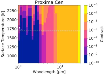
Considering the spectra shown in Figures 8 and 10, we expect a strong influence of the surface temperature (more specifically the Tsurf∕T𝜀ratio) on the detectability of young exoplanets currently in the magma ocean stage. In order to better quantify this detectability, we define the spectral thermal contrast Ciin one of our 36 spectral bands as Ci=(Rp∕R∗)2OLRi∕⟨B(T∗)⟩i, where Rpand R∗stand, respectively, for the planet and the host star radii, OLRifor the planet OLR in a given wave number band, and⟨B(T∗)⟩ithe Planck function averaged upon the same wave number band for the star temperature T∗—that is, assuming that the host star behaves as a blackbody. This contrast underestimates the actual contrast since it does not take into account the reflected stellar component that should be present except for a 180∘ phase angle (e.g., during a primary stellar transit). Results are shown for an Earth-sized planet with a 300 bar −H2O, 100 bar −CO2atmosphere around a solar analog (R∗ = 109.2Rp, T∗ = 5772 K, Figure 11) and a red dwarf similar to Proxima Centauri (R∗ = 15.4Rp,
T∗= 3042 K, Figure 12). The comparison between both plots shows that the contrast is very much improved for a smaller and cooler star, the larger size of the planet relative to its host star more than offsets the shift of the stellar radiation toward longer wavelengths.
Figure 10. Thermal emission spectrum for the atmosphere shown in Figure 9. Dotted lines stand for Planck functions at
Figure 11. Spectral contrast of the thermal emission of an Earth-sized planet with a 300 bar H2O, 100 bar-CO2 atmosphere orbiting against a Sun-like star with respect to surface temperature.T𝜀≈ 1690K is indicated.
There are two considerations to keep in mind when discussing these contrasts. The first consideration deals, obviously, with the instrumental capabilities available as of 2017 or in the foreseeable future. For example, James Webb Space Telescope (JWST) capabilities as stated by Clampin [2011] gives a minimal contrast in the 10−6–10−4range for direct imaging in the near to middle IR. For a single 1 h transit, the expected JWST photon noise of a M dwarf near 4μm at a spectral resolution R ∼ 10 is close to 10−5at 10 pc [Turbet et al., 2016, their Figure 14] and decreases with the inverse of the distance. This photon noise would also decrease as the inverse square root of the number of recorded transits, so that for transits also, the 10−6to 10−4appears a realistic range for our sensitivity. The other, more subtle consideration, deals with the specificity of a detection: are we able to distinguish the thermal emission of a magma ocean planet from the emission of a cooler, older telluric planet?
From the contrasts shown in Figures 11 and 12, it then appears that the highest contrast values (around 10−5 for the Sun,>10−4for Proxima) are reached for𝜆 > 10μm. Although well within the range of detectability in the case of a red dwarf star (but only marginally for a Sun-like star), the emission for these longer wavelengths is not very distinctive with respect to surface temperature since emission always originates from the relatively cool mesosphere. Spectral signatures are most distinctive in the spectral windows that “open up” for Tsurf> T𝜀, but these windows lie in the near IR range where the star is much brighter than the planet, thus hamper-ing the resulthamper-ing contrast, especially for a relatively hot star like the Sun. Therefore, the best diagnostic band is the longest-wavelength spectral window, located in the 3.55–4 μm range (with the 2–2.3 μm band as a
Figure 12. Spectral contrast of the thermal emission of an Earth-sized planet with a 300 bar H2O, 100 bar CO2 atmosphere orbiting against a Proxima Centauri-like star with respect to surface temperature.T𝜀≈ 1690K is indicated.
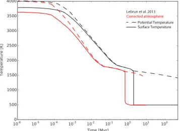
Figure 13. Comparison between the corrected version of the coupled model (in red) and the results of Lebrun et al.
[2013] (in black) for a typical run (their Figure 2i, with a planet-Sun distance of 1 AU,1.435 × 10−2wt % of CO 2and
4.3 × 10⁻²wt % of H
2O). The solid curves stand for the surface temperatures and the dashed curves for the mantle
potential temperatures. The sharp drop in surface temperature indicated that OLR drops below the Nakajima’s limit. Therefore, mantle surface can solidify and condensation of an overlying water ocean may occur afterward.
distant second) in a dense H2O-CO2atmosphere. Although detection of the planet emission within this band is unlikely even for a very hot magma ocean planet around a Sun-like star, it would be well within JWST capa-bilities if a such a magma ocean planet were to orbit a red dwarf within a few hundred parsecs. This optimistic conclusion should however be mitigated by the fact that a Hamano-type I magma ocean planet typically spends less than 105years with T
surf> T𝜀(see section 3.4), thus drastically limiting the detection time
win-dow of such planets. Hamano-type II planets, located close enough to their host stars so that they can reach radiative balance with Tsurf> T𝜀, would remain much longer above the detection threshold, only limited by
the gradual escape of their atmospheres, which results in a secular decline of T𝜀and therefore of Tsurfover mil-lions of years. Finally, it is noteworthy that the only planets that we can hope to detect through their thermal radiation are hot enough (Tsurf> T𝜀) to radiate in their NIR windows regardless of their expected cloud cover according to our cloud model, since these clouds lie at such high altitudes to be optically thin in the NIR range.
3.4. Coupled Evolution of the Atmosphere and Magma Ocean
The atmospheric code developed by Marcq [2012] was one of the building blocks of the model developed by Lebrun et al. [2013] to study the coupled evolution of the atmosphere and magma ocean (MO) of an Earth-sized planet. We therefore checked how its results could be influenced by this update to the atmo-spheric model and correction of the OLR calculation. Figure 13 presents a comparison of the potential and surface temperatures calculated by the two versions of the code, for the conditions shown in Lebrun et al. [2013, their Figure 3i]. Only the cooling time scale differs between the two versions: in the new updated ver-sion, the MO cools down faster but reaches the same temperature at the end of the liquid MO phase. The MO solidification is accelerated by a factor of about 2.5 (8⋅105versus 2⋅106years, respectively), which is consistent with the fact that the corrected NL is now about twice the value from Marcq [2012]. However, this significant correction does not challenge the results about the surface conditions at the end of the MO phase obtained by Lebrun et al. [2013]. Their conclusions about the existence of two types of planets, one condensing water at the end of the MO phase and the other remaining too hot to do so (so-called Hamano-type I and type II planets) are therefore still valid. More results will be presented by Salvador et al. [2017], notably extending the range of investigated volatile inventories.
4. Discussion
4.1. Limitations
Our model is already functional and can be applied to a wide range of planetary atmospheres. There are however some caveats that should be kept in mind before applying this model beyond its validity domain.
4.1.1. Spherical Corrections
When modeling very hot atmospheres (Tsurf> 2500 K) around smaller (Mars-sized) telluric planets, we find that the atmospheric scale height H is not negligible compared to the planetary radius R. This challenges the
common plane-parallel assumption of most models, including ours. However, some corrections can solve or at least alleviate these potential sphericity issues.
First, hydrostatic equilibrium itself is unaffected by sphericity (1-D spherical gradient is𝜕P∕𝜕r instead of
𝜕P∕𝜕z in Cartesian coordinates), but the straightfoward relation between surface pressure and atmospheric
mass needed by interior models [Lebrun et al., 2013; Salvador et al., 2017] is lost. However, numerical radial integration of the density profile is straightforward and yields the required volatile mass.
Adaptations to the radiative transfer code are more complex. We found no publicly available 1-D spherical radiative transfer codes similar to DISORT; Rannou et al. [2010] however provided us with a pseudospherical adaptation of DISORT that takes spherical geometry into consideration only for the incident and emerging beams. This could be used in a future version of our model, provided the mean free path of photons is small compared to the planetary radius. In such a case, a first-order approximation could be to correct the OLR—in W/m2, the area being understood at the planetary surface—for the actual altitude where the thermal radi-ation originates. One way to do so, especially in the case of negligible scattering, would be, for each g bin in the k-correlated code, to locate the altitude zgwhere the physical temperature is equal to the brightness temperature (as computed with the plane-parallel radiative code), and weighting the corresponding spectral flux by(1 + zg2∕R2
)
before integration on the g space. This would enhance the OLR, as well as lead to less intuitive consequences if the effective altitude of thermal emission differs significantly from, e.g., the effec-tive altitude for the absorption of the stellar component (see section 4.1.2). Similar arguments are developed by Goldblatt [2015], and result in an OLR enhancement on the order of 10 W/m2for pure steam atmospheres around Earth-sized planets (up to 30 W/m2for Mars-sized planets).
A last spherical correction would deal with the mesospheric temperature: if we eventually compute it through canceling the divergence of the OLR + absorbed stellar flux at vanishing optical depth, we must keep in mind that the radial divergence operator in spherical coordinates is not identical to the vertical divergence in Carte-sian coordinates (unlike the vertical and radial gradients discussed earlier in this section). The net effect would be a cooling of the mesosphere—the outer surface of the topmost spherical shell cooling to space being larger than the inner surface heated from below in spherical geometry, but the exact extent of this extra cooling is yet to be quantified.
4.1.2. Radiative Shortcomings
As already mentioned before (section 3.2.2), we need in the near future to extend the radiative transfer calcu-lations to shorter wavelengths whenever considering very hot surfaces surrounded with comparatively light atmospheres—this was already highlighted and extensively discussed by Marcq [2012]. Such an extension would encompass visible and near UV (up to 35,000 cm−1) so that we could model absorption and scattering of the stellar component for stars in the G, K, and M spectral classes.
Incidentally, the inclusion of shorter wavelengths in our thermal radiative transfer calculations would solve a possible issue in the case of very hot surfaces under very thin atmospheres, where thermal radiation shortward of 1μm is expected to be significant. However, this is not the case in the parameter space covered in this paper: graphical integration performed upon Hamano et al. [2015, their Figure 1a] spectrum shows that for a relatively hot 2500 K surface under a relatively thin 50 bar pure steam atmosphere, OLR shortward of 1μm only accounts for less than 5% of the total OLR.
This inclusion would yield considerable improvements in our model, namely, (1) a true computation of the spectral and bolometric albedo of these atmospheres using the existing radiative transfer code and (2) as a consequence, open the possibility to improve the computation of the T(p) profile in the upper radiative layers of the atmosphere better than the current isothermal assumption. Of course, Rayleigh scattering would have to be added to the Mie scattering which is the only one considered in the current stage of the model. Spherical corrections to the stellar component of the radiative transfer would be similar to what is proposed in section 4.1.1: weighting in each g bin according to the altitude of effective scattering, defined by a nadir optical depth̄𝜏scat =𝜛0
[
3(1 −𝜛0 )]−1∕2
in an analytical semi-infinite two-stream solution, where𝜛0is the single scattering albedo.
5. Conclusion
Our updated model mostly confirms the qualitative findings from Marcq [2012] and comparable studies such as Hamano et al. [2013]. Including this updated model into the coupled model of Lebrun et al. [2013] also
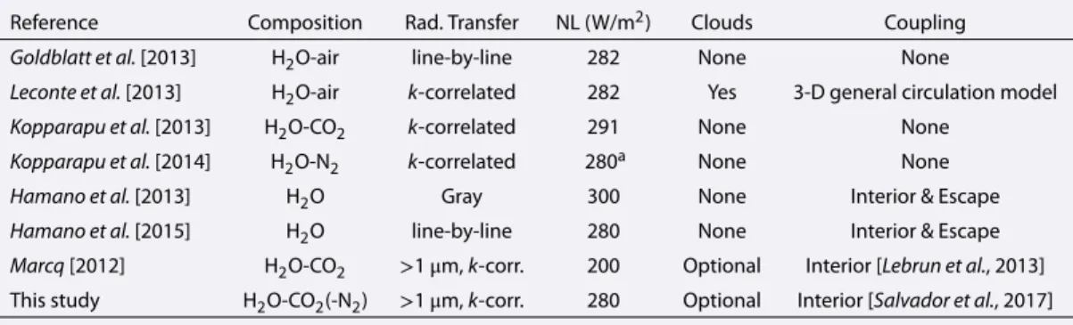
Table 1. Comparison Between Recent H2O-Rich Atmospheric Models
Reference Composition Rad. Transfer NL (W/m2) Clouds Coupling
Goldblatt et al. [2013] H2O-air line-by-line 282 None None
Leconte et al. [2013] H2O-air k-correlated 282 Yes 3-D general circulation model
Kopparapu et al. [2013] H2O-CO2 k-correlated 291 None None
Kopparapu et al. [2014] H2O-N2 k-correlated 280a None None
Hamano et al. [2013] H2O Gray 300 None Interior & Escape
Hamano et al. [2015] H2O line-by-line 280 None Interior & Escape
Marcq [2012] H2O-CO2 >1μm,k-corr. 200 Optional Interior [Lebrun et al., 2013]
This study H2O-CO2(-N2) >1μm,k-corr. 280 Optional Interior [Salvador et al., 2017]
aFor an Earth-mass planet.
confirms its qualitative behavior, as can be seen in Figure 13. The main correction deals with the new estima-tion of Nakajima’s limit in the clear sky case around 280 W/m2, much better in line with comparable recent work (Table 1). The improved numerical stability and switch to an adaptative p grid instead of a fixed z grid also enabled the investigation of a broader input parameter space, so that we could derive an analytic param-eterization of the threshold blanketing temperature (defined as the surface temperature where the effective emissivity peaks) with respect to the surface pressures of H2O and CO2. The new updated coupled model is used by Salvador et al. [2017] to systematically investigate the influence of volatile content on the inner limit of water condensation at the end of the magma ocean phase.
We can also model the effect of a 100%, thick cloud cover, leading to a reduction of the OLR by up to 40% and a raise of about 10% of the threshold blanketing temperature. However, since a proper model of the cloud cover requires a more sophisticated 3-D model like in Leconte et al. [2013], we chose to focus most of our studies on the cloudless case. Current limitations (near IR cutoff, plane-parallel assumption, and lack of stellar radiative transfer) and some hints about how to overcome them were also discussed.
These updates to the model of Marcq [2012] are best understood in the context of recent comparable work for H2O-rich atmospheres, whether around magma ocean planets or for runaway greenhouse studies (see Table 1). Their similarities, far from being redundant, enable detailed cross comparison and provide useful benchmarking during the development or adaptation of new models. We can also see that no model is supe-rior in all points to the others: they all have different strengths and weaknesses, which enables any final user developing their own coupled atmosphere-interior-escape model to select the one best suited to their needs.
References
Abe, Y., and T. Matsui (1988), Evolution of an impact-generated H2O-CO2atmosphere and formation of a hot proto-ocean on Earth,
J. Atmos. Sci., 45, 3081–3101, doi:10.1175/1520-0469(1988)045<3081:EOAIGH>2.0.CO;2.
Bézard, B., A. Fedorova, J.-L. Bertaux, A. Rodin, and O. Korablev (2011), The 1.10- and 1.18-μm nightside windows of Venus observed by SPICAV-IR aboard Venus Express, Icarus, 216, 173–183, doi:10.1016/j.icarus.2011.08.025.
Chase, M. (1998), Nist-JANAF Thermochemical Tables, Am. Chem. Soc., Washington, D. C.
Clampin, M. (2011), The James Webb space telescope and its capabilities for exoplanet science, in The Astrophysics of Planetary Systems:
Formation, Structure, and Dynamical Evolution, IAU Symposium, vol. 276, edited by A. Sozzetti, M. G. Lattanzi, and A. P. Boss, pp. 335–342,
Cambridge Univ. Press, Cambridge, U. K., doi:10.1017/S1743921311020400.
Clough, S. A., M. W. Shephard, E. J. Mlawer, J. S. Delamere, M. J. Iacono, K. Cady-Pereira, S. Boukabara, and P. D. Brown (2005), Atmospheric radiative transfer modeling: A summary of the AER codes, J. Quant. Spectrosc. Radiat. Transfer, 91, 233–244, doi:10.1016/j.jqsrt.2004.05.058.
Elkins-Tanton, L. T. (2008), Linked magma ocean solidification and atmospheric growth for Earth and Mars, Earth Planet. Sci. Lett., 271, 181–191, doi:10.1016/j.epsl.2008.03.062.
Eymet, V., C. Coustet, and B. Piaud (2016), KSPECTRUM: An open-source code for high-resolution molecular absorption spectra production,
J. Phys. Conf. Ser., 676(1), 12005, doi:10.1088/1742-6596/676/1/012005.
Goldblatt, C. (2015), Habitability of waterworlds: Runaway greenhouses, atmospheric expansion, and multiple climate states of pure water atmospheres, Astrobiology, 15, 362–370, doi:10.1089/ast.2014.1268.
Goldblatt, C., T. D. Robinson, K. J. Zahnle, and D. Crisp (2013), Low simulated radiation limit for runaway greenhouse climates, Nat. Geosci., 6, 661–667, doi:10.1038/ngeo1892.
Haar, L., J. Gallagher, G. Kell, and National Standard Reference Data System (U.S.) (1984), NBS/NRC Steam Tables: Thermodynamic and
Transport Properties and Computer Programs for Vapor and Liquid States of Water in SI Units, Hemisphere Publ. Corp., Washington, D. C.
Hamano, K., Y. Abe, and H. Genda (2013), Emergence of two types of terrestrial planet on solidification of magma ocean, Nature, 497, 607–610, doi:10.1038/nature12163.
Hamano, K., H. Kawahara, Y. Abe, M. Onishi, and G. L. Hashimoto (2015), Lifetime and spectral evolution of a magma ocean with a steam atmosphere: Its detectability by future direct imaging, Astrophys. J., 806, 216, doi:10.1088/0004-637X/806/2/216.
Acknowledgments
We wish to thank M. Turbet, J. Leconte, C. Goldblatt, and F. Selsis for fruitful scientific discussions while presenting this model. The authors have been supported by a grant from the Programme National de Planétologie (PNP) sponsored by the Institut National des Sciences de l’Univers (INSU). Arnaud Salvador’s PhD is supported by a grant from the Ministère de la Recherche and Université Paris Sud. Data policy: the source code of this model can be downloaded here: http://marcq. page.latmos.ipsl.fr/radconv1d.html.
Ingersoll, A. P. (1969), The runaway greenhouse: A history of water on Venus, J. Atmos. Sci., 26, 1191–1198, doi:10.1175/1520-0469(1969)026<1191:TRGAHO>2.0.CO;2.
Kasting, J. F. (1988), Runaway and moist greenhouse atmospheres and the evolution of Earth and Venus, Icarus, 74, 472–494, doi:10.1016/0019-1035(88)90116-9.
Komabayashi, M. (1967), Discrete equilibrium temperatures of a hypothetical planet with the atmosphere and the hydrosphere of one component-two phase system under constant solar radiation, J. Meteorol. Soc. Jpn., 45, 137–139.
Kopparapu, R. K., R. Ramirez, J. F. Kasting, V. Eymet, T. D. Robinson, S. Mahadevan, R. C. Terrien, S. Domagal-Goldman, V. Meadows, and R. Deshpande (2013), Habitable zones around main-sequence stars: New estimates, Astrophys. J., 765, 131, doi:10.1088/0004-637X/765/2/131.
Kopparapu, R. K., R. M. Ramirez, J. SchottelKotte, J. F. Kasting, S. Domagal-Goldman, and V. Eymet (2014), Habitable zones around main-sequence Stars: Dependence on planetary mass, Astrophys. J. Lett., 787, L29, doi:10.1088/2041-8205/787/2/L29.
Kopparapu, R. k., E. T. Wolf, J. Haqq-Misra, J. Yang, J. F. Kasting, V. Meadows, R. Terrien, and S. Mahadevan (2016), The inner edge of the habitable zone for synchronously rotating planets around low-mass stars using general circulation models, Astrophys. J., 819, 84, doi:10.3847/0004-637X/819/1/84.
Lebrun, T., H. Massol, E. Chassefière, A. Davaille, E. Marcq, P. Sarda, F. Leblanc, and G. Brandeis (2013), Thermal evolution of an early magma ocean in interaction with the atmosphere, J. Geophys. Res. Planets, 118, 1155–1176, doi:10.1002/jgre.20068.
Leconte, J., F. Forget, B. Charnay, R. Wordsworth, and A. Pottier (2013), Increased insolation threshold for runaway greenhouse processes on Earth-like planets, Nature, 504, 268–271, doi:10.1038/nature12827.
Lupu, R. E., K. Zahnle, M. S. Marley, L. Schaefer, B. Fegley, C. Morley, K. Cahoy, R. Freedman, and J. J. Fortney (2014), The atmospheres of Earthlike planets after giant impact events, Astrophys. J., 784, 27, doi:10.1088/0004-637X/784/1/27.
Ma, Q., and R. H. Tipping (1992), A far wing line shape theory and its application to the foreign-broadened water continuum absorption. III,
J. Chem. Phys., 97, 818–828, doi:10.1063/1.463184.
Marcq, E. (2012), A simple 1-D radiative-convective atmospheric model designed for integration into coupled models of magma ocean planets, J. Geophys. Res., 117, E01001, doi:10.1029/2011JE003912.
Marcq, E., B. Bézard, P. Drossart, G. Piccioni, J. M. Reess, and F. Henry (2008), A latitudinal survey of CO, OCS, H2O, and SO2in the lower atmosphere of Venus: Spectroscopic studies using VIRTIS-H, J. Geophys. Res., 113, E00B07, doi:10.1029/2008JE003074.
Nakajima, S., Y.-Y. Hayashi, and Y. Abe (1992), A study on the ’runaway greenhouse effect’ with a one-dimensional radiative-convective equilibrium model, J. Atmos. Sci., 49, 2256–2266, doi:10.1175/1520-0469(1992)049<2256:ASOTGE>2.0.CO;2.
Rannou, P., T. Cours, S. Le Mouélic, S. Rodriguez, C. Sotin, P. Drossart, and R. Brown (2010), Titan haze distribution and optical properties retrieved from recent observations, Icarus, 208, 850–867, doi:10.1016/j.icarus.2010.03.016.
Salvador, A., H. Massol, A. Davaille, E. Marcq, P. Sarda, and E. Chassefière (2017), The relative influence of H2O and CO2on the primitive surface conditions and evolution of rocky planets, J. Geophys. Res. Planets, 122, doi:10.1002/2017JE005286.
Schaefer, L., R. D. Wordsworth, Z. Berta-Thompson, and D. Sasselov (2016), Predictions of the atmospheric composition of GJ 1132b,
Astrophys. J., 829, 63, doi:10.3847/0004-637X/829/2/63.
Stamnes, K., S.-C. Tsay, K. Jayaweera, and W. Wiscombe (1988), Numerically stable algorithm for discrete-ordinate-method radiative transfer in multiple scattering and emitting layered media, Appl. Opt., 27, 2502–2509, doi:10.1364/AO.27.002502.
Turbet, M., J. Leconte, F. Selsis, E. Bolmont, F. Forget, I. Ribas, S. N. Raymond, and G. Anglada-Escudé (2016), The habitability of Proxima Centauri b. II. Possible climates and observability, Astrono. Astrophys., 596, A112, doi:10.1051/0004-6361/201629577.
Wordsworth, R. D., and R. T. Pierrehumbert (2013), Water loss from terrestrial planets with CO2-rich atmospheres, Astrophys. J., 778, 154, doi:10.1088/0004-637X/778/2/154.
Yang, J., and D. S. Abbot (2014), A low-order model of water vapor, clouds, and thermal emission for tidally locked terrestrial planets,
Astrophys. J., 784, 155, doi:10.1088/0004-637X/784/2/155.
Yang, J., N. B. Cowan, and D. S. Abbot (2013), Stabilizing cloud feedback dramatically expands the habitable zone of tidally locked planets,
Astrophys. J. Lett., 771, L45, doi:10.1088/2041-8205/771/2/L45.
Yang, J., G. Boué, D. C. Fabrycky, and D. S. Abbot (2014), Strong dependence of the inner edge of the habitable zone on planetary rotation rate, Astrophys. J. Lett., 787, L2, doi:10.1088/2041-8205/787/1/L2.