HAL Id: insu-02571753
https://hal-insu.archives-ouvertes.fr/insu-02571753
Submitted on 13 May 2020
HAL is a multi-disciplinary open access
archive for the deposit and dissemination of sci-entific research documents, whether they are pub-lished or not. The documents may come from teaching and research institutions in France or abroad, or from public or private research centers.
L’archive ouverte pluridisciplinaire HAL, est destinée au dépôt et à la diffusion de documents scientifiques de niveau recherche, publiés ou non, émanant des établissements d’enseignement et de recherche français ou étrangers, des laboratoires publics ou privés.
Combining fiber optic DTS, cross-hole ERT and
time-lapse induction logging to characterize and monitor
a coastal aquifer
A. Folch, L. del Val, Linda Luquot, L. Martínez-Pérez, F. Bellmunt, H. Le
Lay, V. Rodellas, N. Ferrer, A. Palacios, S. Fernandez, et al.
To cite this version:
A. Folch, L. del Val, Linda Luquot, L. Martínez-Pérez, F. Bellmunt, et al.. Combining fiber optic DTS, cross-hole ERT and time-lapse induction logging to characterize and monitor a coastal aquifer. Journal of Hydrology, Elsevier, 2020, 588, pp.125050. �10.1016/j.jhydrol.2020.125050�. �insu-02571753�
Journal Pre-proofs
Research papers
Combining fiber optic DTS, cross-hole ERT and time-lapse induction logging to characterize and monitor a coastal aquifer
A. Folch, L. del Val, L. Luquot, L. Martínez-Pérez, F. Bellmunt, H. Le Lay, V. Rodellas, N. Ferrer, A. Palacios, S. Fernández, M.A. Marazuela, M. Diego-Feliu, M. Pool, T. Goyetche, J. Ledo, P. Pezard, O. Bour, P. Queralt, A. Marcuello, J. Garcia-Orellana, M.W. Saaltink, E. Vazquez-Suñe, J. Carrera
PII: S0022-1694(20)30510-2
DOI: https://doi.org/10.1016/j.jhydrol.2020.125050
Reference: HYDROL 125050
To appear in: Journal of Hydrology
Received Date: 2 August 2019
Revised Date: 22 April 2020
Accepted Date: 4 May 2020
Please cite this article as: Folch, A., del Val, L., Luquot, L., Martínez-Pérez, L., Bellmunt, F., Le Lay, H., Rodellas, V., Ferrer, N., Palacios, A., Fernández, S., Marazuela, M.A., Diego-Feliu, M., Pool, M., Goyetche, T., Ledo, J., Pezard, P., Bour, O., Queralt, P., Marcuello, A., Garcia-Orellana, J., Saaltink, M.W., Vazquez-Suñe, E., Carrera, J., Combining fiber optic DTS, cross-hole ERT and time-lapse induction logging to characterize and monitor a coastal aquifer, Journal of Hydrology (2020), doi: https://doi.org/10.1016/j.jhydrol.2020.125050
This is a PDF file of an article that has undergone enhancements after acceptance, such as the addition of a cover page and metadata, and formatting for readability, but it is not yet the definitive version of record. This version will undergo additional copyediting, typesetting and review before it is published in its final form, but we are providing this version to give early visibility of the article. Please note that, during the production process, errors may be discovered which could affect the content, and all legal disclaimers that apply to the journal pertain.
Combining fiber optic DTS, cross-hole ERT and time-lapse induction logging to characterize and monitor a coastal aquifer.
Folch, A.1,2,*, L. del Val1,2, L. Luquot3,4,2, L. Martínez-Pérez1,2,3, F. Bellmunt5, H. Le Lay7, V.
Rodellas8, N. Ferrer1,2, A. Palacios1,2,3, S. Fernández1,2,3, M. A. Marazuela1,2,3, M. Diego-Feliu8, M.
Pool3,2, T. Goyetche1,2,3, J. Ledo5, P. Pezard4, O. Bour6, P. Queralt5, A. Marcuello5, J.
Garcia-Orellana8,9, M.W. Saaltink1,2, E. Vazquez-Suñe3,2 and J. Carrera3,2
1 Department of Civil and Environmental Engineering (DECA), Universitat Politécnica de Catalunya,
Barcelona, Spain.
2 Associated Unit: Hydrogeology Group (UPC-CSIC).
3 Institute of Environmental Assessment and Water Research, CSIC, Barcelona, Spain 4 Laboratoire Géosciences Montpellier, UMR 5243, Montpellier, France.
5 Institut de Recerca Geomodels, Universitat de Barcelona, Spain.
6 Univ Rennes, CNRS, Géosciences Rennes, UMR 6118, 35000 Rennes, France. 7UMR SAS, Agrocampus Ouest, INRA, 35000 Rennes, France
8 Departament de Física, Universitat Autònoma de Barcelona, Bellaterra, Spain.
9 Institut de Ciència i Tecnologia Ambiental (ICTA-UAB), Universitat Autònoma de Barcelona, Bellaterra,
Spain.
* Serra Hunter Fellow /Corresponding author
Keywords: cross hole electrical resistivity tomography, fiber optic distributed temperature
sensing, formation electrical conductivity, sea water intrusion, submarine groundwater discharge, alluvial aquifer
1. Introduction
About 41% of the world population lives in coastal areas (Martínez et al., 2007), where groundwater is the main source of freshwater. Intensive groundwater exploitation has caused seawater intrusion (SWI) in the past decades, bore and soil salinization with important losses in agricultural production globally. Moreover, the impact and magnitude of SWI is expected to be exacerbated by the increase in the freshwater demand due to the population growth, as well as by climate change and sea-level rise. Much progress has been made to characterize SWI in coastal aquifers and to understand the reactions occurring in the reactive mixing zone between terrestrial groundwater and seawater (i.e. subterranean estuary; Anwar et al., 2014; Moore, 2010, 1999; O’Connor et al., 2015; Santos et al., 2009; Spiteri et al., 2008). However, the understanding of the dynamics of mixing and dispersion and its impact on chemical reactions remains a challenge.
Transport processes in coastal aquifers have recently received increasing attention, particularly in relation to the threat of SWI as well as the complex aquifer-ocean interactions. Density-driven circulation significantly affects dispersion, mixing, and reaction behavior of nutrients and contaminants transported by freshwater, and thus, the supply of these compounds to the coastal sea (Brovelli et al., 2007; Dror et al., 2003). The discharge of groundwater to the sea, commonly referred to as submarine groundwater discharge (SGD), has been recognized as a relevant source of dissolved nutrients (Kim et al., 2011; Rodellas et al., 2015) and metals to the ocean (e.g. (Bone et al., 2007; Trezzi et al., 2017; Windom et al., 2006) with important implications for coastal areas. Therefore, quantification of fluxes between coastal aquifers and oceans is critically important, both from a hydrogeological and oceanographic perspective. However, while studying the same process and addressing the same key questions, these two communities have evolved independently.
Fluctuations on the fresh-saltwater interface location and width depend on many factors (e.g. recent and past freshwater inputs, permeability of the aquifer, sea-level, and tidal range). The complexity of coastal systems under natural dynamics is aggravated by global change (e.g. sea-level rise, changes in precipitation, increased urbanization in coastal areas, increase on the demand of hydrological resources, etc.) (Michael et al., 2017; Rufí-Salís et al., 2019). The predicted climate change with its associated sea-level rise will modify flow regimes and groundwater discharge conditions in many coastal areas. All these changes and interactions will affect the inland extension and behaviour of SWI as well as the chemical composition and magnitude of SGD. Additionally, despite the transient behaviour of SWI, its current understanding is mainly based on studies that assume steady-state conditions (Werner et al., 2013), and thus implicitly neglect the transient effects and processes that are occurring at different temporal and spatial scales, such as quality patterns (mixing, cation exchange and/or precipitation/dissolution of different minerals). Furthermore, the behaviour of SWI differs between passive and active SWI (Badaruddin et al., 2015; Werner, 2017), and rain events can also have an important influence in the dynamics of these systems at day time-scale (Cerdà-Domènech et al., 2017; Giambastiani et al., 2017).
The dynamics of the SWI can also be affected by other factors offshore, such as beach geomorphology, tidal regime, wave action and the flux of fresh groundwater that discharges offshore (Michael et al., 2005). Moreover, the structure of the aquifer plays an important role in specific contexts, where the presence of low permeable layer as thin as a few decimeters may form a confining layer dividing the system in two aquifers and modifying the dynamics of the system (Pauw et al., 2017). This kind of lithological structure with a low permeable layer changes the behaviour of the SWI and modifies the way in which groundwater discharges into the sea. Furthermore, layered aquifer systems may exhibit enhanced seasonal exchange due to an increase in the length of the fresh-saltwater interface (Michael et al., 2005). Therefore, due to
the importance of lithological variability on groundwater flow and salinity patterns, detailed field studies are needed to understand these interactions (Pauw et al., 2017).
Traditional methods to characterize inland aquifers are also used to depict groundwater systems in coastal areas. Direct information is obtained from piezometers where hydraulic head, physicochemical parameters and isotopes are measured/sampled to study the SWI and coastal groundwater systems (Re et al., 2014 among others). However, as was stated already by Post in 2005, in order to successfully apply existing and future models that describe three-dimensional flow, transport and geochemical interaction under variable density conditions, a detailed and accurate characterization of the subsurface is required. In recent years, there have been many new techniques focused on this. characterization, which are summarized below.
Due to the correlation between water salinity and bulk or formation electrical conductivity, electrical methods such as electromagnetic methods and electrical resistivity tomography (ERT) represent are interesting tools to monitor SWI. Induction logging can also be used to effectively detect and monitor the saltwater wedge at the meter scale and in the near field around boreholes (Denchik et al., 2014; Garing et al., 2013; Pezard et al., 2015). ERT is widely used for hydrological purposes, such as monitoring contaminant plume migration or estimation of aquifer parameters (Camporese et al., 2011; Cassiani et al., 2006; Koestel et al., 2008; Müller et al., 2010; Nguyen et al., 2009; Perri et al., 2012; Singha et al., 2015 among others). Some examples of its successful application to image the freshwater-saltwater interface in different coastal areas are described by de Franco et al., 2009; Goebel et al., 2017; Morrow et al., 2010; Nguyen et al., 2009; and Zarroca et al., 2014. Nevertheless, although widely used, the sensitivity of the ERT measurements depends on the acquisition methodology. One of the most widespread method consists on positioning the electrodes on the surface. The resolution under this configuration decreases as the acquisition depth increase, preventing the quantitative use of the data from a hydrogeological perspective. An alternative method consists of installing the
electrodes along the piezometers, which contributes having better resolution acquisitions (Perri et al., 2012). Attempts to link bulk electrical conductivity obtained using surface or surface-to-borehole ERT are found in the literature (Beaujean et al., 2017; Huizer et al., 2017; Nguyen et al., 2009). These studies concluded that ERT-derived water salinity is usually underestimated. Therefore, attaching electrodes around and along the piezometers, allows to acquire data near the area of interest and cross-hole, limiting the loss of resolution in depth.
Temperature can also be used as a tracer of environmental processes in groundwater using the temperature contrast between two end-members. Fiber optic distributed temperature sensing (FO-DTS) has already proven to be a useful cost-effective tool to perform detailed monitoring of environmental processes (Selker et al., 2006; Tyler et al., 2009). At present, FO-DTS instruments provide temperature resolution of 0.01ºC, a spatial sampling of 0.25 m along the cable and a temporal resolution of fractions of a minute depending on the configuration chosen (Selker et al., 2006, Simon et al. 2020). The application of this technology in groundwater environments, has been used in both fractured media and unconsolidated aquifers to determine river-aquifer interaction (Briggs et al. 2016; Rosenberry et al.2016), evaluate groundwater preferential paths, identify fracture connectivity, and approximate aquifer hydraulic and thermal properties (Bakker et al., 2015; Bense et al. 2016; Hausner et al., 2016; Klepikova et al., 2014). In coastal aquifers, temperature may be a good indicator for mixing due to the different temperatures of fresh groundwater and seawater. Based on this contrast, Taniguchi (2000) used temperature as a proxy to monitor dynamics in the fresh-saltwater interface at a coastal aquifer in Japan. The same principle was used by Debnath et al., (2015) and Henderson et al., (2008) to monitor interactions between groundwater and sea water using temperature probes and distributed temperature sensing (DTS) respectively. Based on these natural differences in temperature, FO-DTS may be used as a passive sensor to monitor the spatial distribution and temporal fluctuations of the fresh-salt water interface with high-definition. Despite some examples that
combine marine ERT and DTS to monitor tidal pumping and SGD (Henderson et al. 2010), FO-DTS has not been applied yet to characterize SWI.
Given the importance of fresh groundwater preservation and the complexity of coastal aquifer settings, it is doubtful that a single technique is enough to understand the whole system. For this reason, we have developed a research site in a Mediterranean alluvial aquifer (North of Barcelona, Catalunya, Spain), between 40 and 90 m from the seashore, to compare the performance of different characterization methods and provide new insights to be shared among the SWI and SGD scientific communities. Unlike most studies conducted elsewhere, the selected area presents a microtidal regime, which allows focusing on other physical driving forces (waves, storms, groundwater table elevation, etc).
In this paper we present the preliminary results of the jointly application of different novel monitoring techniques with the objective to evaluate temporal variations of a coastal aquifer at different spatial scales. At the site scale, the selected techniques are: 1) Cross-hole electrical resistivity tomography (CHERT) and 2) FO-DTS, as a first attempt to apply this technique to characterize SWI. At meter/borehole scale, for the first time according to the authors knowledge, we deployed a time lapse induction logging (TILL) with an electromagnetic probe to obtain formation conductivity logs at relatively high frequency (one sample every ten minutes) to study aquifer processes at these time scales. These techniques are compared with traditional measures in piezometers (electrical conductivity and temperature) and applied to obtain two snapshots at different times to characterize the beginning and the end of the dry season (June and September 2015).
2. Experimental site
the urban areas of Mataró and Vilassar de Mar (Figure 1). The area is subjected to a Mediterranean semi-arid climate with an average annual precipitation of 610 mm (period 2010-2013). The land use is manly divided into agriculture and urban and natural forest (Rufí-Salís et al., 2019). The watercourse is characterized by torrential and non-permanent water flow, which only develops after heavy rain events.
Figure 1. Location and pilot site setup in the NW Mediterranean basin. a) Maps depicting the location of the field site with respect to the surrounding water bodies and infrastructures. b) Map showing the distribution of the installed piezometers at the experimental site. The color scale indicates the depth of the screened section of each borehole. The red line depicts the position of the vertical cross-sections shown throughout the article, from A (inland) to B (seawards).
The site is located in the lower part of the Argentona stream alluvial aquifer. The geology of the experimental site is dominated by layers of quaternary gravels, sands and clays which are the product of the weathering of the surrounding granitic outcrops (Figure 2) (Martínez-Pérez et al. 2018, Internal communication).
In a distance of 30 to 90 m from the seashore, 16 shallow piezometers were installed in a small area of 30 by 20 meters, 30 m inland from the seashore. Most piezometers are gathered in nests (N1, N2, N3 and N4) of three (15, 20, 25), with depths of around 15, 20 and 25 m (e.g. nest N1 is composed of piezometers N115, N120 an N125). Four stand-alone piezometers were also
piezometers were equipped with at least 2 m of blind pipe at the bottom, followed by 2 m of screened tube just above. The only exceptions were piezometers PP15 and PP20, which were screened 11 and 15 m respectively. The study presented here focuses on a cross-section perpendicular to the sea following the piezometers N225, N325, N125, PP15 and PP20 (Figure 2).
Figure 2. Cross section of the experimental site perpendicular to the seashore (Figure 1b). The different color lines represent the contact between weathered granite and the alluvial formation (red) and between the anthropic materials and the alluvial sediments (Brown). Black lines represent the correlation between fine materials levels in the different piezometers integrating gamma log data for all boreholes (data not shown). Grey layer indicates a continuous layer of silt that crosses all piezometers.
3. Methodology
The methodology described below describes the two stages of the study: (1) initial downhole set-up of both FO-DTS and the distribution of electrodes to perform CHERT, and (2) field surveys of FO-DTS, CHERT and time-lapse induction logging.
3.1. Installation of annulus fiber optic cable and electrodes during site construction
The fiber optic cable (Brugg Kabel AG, Switzerland) and CHERT electrodes lines were placed during piezometers installation in the annular space between the PVC casing and the formation. The procedure consisted of three steps: (1) electrodes assembly; (2) installing the electrodes along the tubing; and (3) fiber optic cable set-up along the piezometer casing (Figure 3).
The assembly of the electrodes aimed at hindering corrosion, since this is one of the main difficulty with semi-permanent electrodes in a saltwater environment. The electrodes, made of stainless steel meshes, were tested in the laboratory by submerging them (and the cables) in a salty solution (55 mS/cm). Then, the electrodes were connected to an electrical cable through which an electrical current was imposed to observe the corrosion. The most sensitive part of the system was the connection between the mesh and the cable. After several tests, we determined that the best strategy to delay corrosion was to fully cover the connection with silicone to minimize the contact with saltwater. The final prototype showed corrosion signs in the laboratory after 20 days of continuous current of 1 A at 3 Hz frequency. The current injected during field experiment is much smaller than 1A and time of injection is only a few mS. This, together with the reducing conditions fonded at the deepest part of the site (Martínez-Pérez et al. 2018, Internal communication), should ensure reliable operation for the foreseeable duration of the project. More details in the CHERT configuration can be found in Palacios et al. 2020. The installation stage consisted of fixing electrodes and fiber optic lines to the casing by means of nylon flanges, which effectively acted as centralizers to protect the two lines (Figure 3). Had the wells been deeper, more sturdy protection and centering system would have been needed. The first casing sections were instrumented outside the well and placed vertically inside the auxiliary drilling tubing with the help of the rig crane. The rest of the casing sections were instrumented just after they had been screwed to the casing string already in place. The casing, thus instrumented, was lowered smoothly into the auxiliary tubing for all piezometers. Special
attention was paid to prevent dragging casing and instrumentation lines during the extraction of the auxiliary tubing. To this end, we tried to minimize the length over which filter sand in the screened interval, or clay pellets elsewhere, overlapped with auxiliary tubing (Figure 3). The whole operation requires the pro-active collaboration of drillers, who were carefully trained on what we were trying to do.
The deepest piezometers of each nest, and the stand-alone piezometers (PP15 and PP20) were equipped with 36 electrodes (Figure 2) to perform both vertical and cross-hole electrical resistivity tomography (CHERT). Distances between electrodes were 40 cm, 50 cm and 68 cm for piezometers with depths of 15 m, 20 m and 25 m, respectively. In the Argentona site, the distance between nests and pumping wells varies from around 10 m to 26 m while the distance between PP20 and P15, the shallowest piezometers equipped with CHERT, is of 12.7 m. In the line perpendicular to the coastline, the CHERT has an aspect ratio (horizontal distance between boreholes divided by depth of boreholes) between 0.6 and 0.8.
In order to perform FO-DTS, fiber optic cables must be installed in all the piezometers of the site. This made it difficult because the cable needed to be cut to extract the auxiliary tubing (Figure 3). The end of the cable was passed through the tubing to minimize the number of cable segments (or fusions) connections, which cause a loss in signal. In hindsight, this has proven a severe hindrance.
The connections between fusions were done with a Prolite-40 Fusion Splicer (PROMAX, Spain) and an EFC-22 fiber optic cutter (Ericson, Sweden). Two continuous lines of fiber optic cable were set up along the site period. Line 1 included wells from nest N1 and N3, and stand-alone wells PP15 and PP20 period. Line 2 included wells PS25, N220, N215, N225. The total length of fiber optic cable installed was of 1,900 m approximately, with 17 connections.
Figure 3. a) Schematic description of piezometer nest monitoring system, including CHERT electrodes (actually, 32 electrodes were installed in each piezometer) and fiber optic cable for DTS. (b) photo of the electrodes and cable installation in the piezometric tube. During extraction of the drilling auxiliary pipe (c), the fiber cable has to be cut, requiring fusion points. The black bar represents the nylon flanges to fix the electrodes and the fiber optic cable on the piezometer.
3.2. Data acquisition
All surveys were performed in 2015. CHERT data were acquired on July 3rd and September 8th in
boreholes N125, N225, N325, PP20 and PP15. Temperature with FO-DTS was measured on June 25th – 26th and September 10th, in all piezometers, for durations spanning between one and four
hours. Time-lapse induction logging (TLIL) were recorded only in borehole N3-20 on May 11th
and 12th. During all field surveys, head levels, groundwater temperature and electrical
conductivity were measured in all piezometers including water EC vertical profiles in PP20 using a CTD-Diver Schlumberger.
CHERT was done in four pairs of piezometers to obtain a cross-section perpendicular to the coastline, from PP20 to N225. The acquisitions were made using 72 electrodes in total. To maximize resolution, the cross-hole configurations used were dipole-dipole, pole-tripole, and Wenner, following Bellmunt et al. (2016) (Figure 4). We used a ten-channel Syscal Pro resistivity meter and an optimized survey design which allowed to record normal and reciprocal measurements: a total of 5842 data points per cross-hole panel in 30 minutes. The recording of a complete CHERT took 2 hours.
Figure 4. Electrode configurations for the acquisition of CHERT. A and B designate the current electrodes, and M and N the potential electrodes. In the cross-hole dipole-dipole array (CH AB-MN), the current electrodes are in the first borehole while potential electrodes are in the second borehole. In the cross-hole pole-tripole array (CH AMN-B/A-BMN), a current is imposed in the two boreholes while potential electrodes are in the same borehole.
CHERT apparent resistivities from July and September 2015 were inverted using the acquisition performed in July as a baseline for the time-lapse inversion. Both datasets were scanned to remove data points with large errors (differences of more than 10% between normal and reciprocal measurements), and compared to keep exactly the same electrode configuration in both acquisitions. For time-lapse inversion, the same set-up was preserved to ensure that the
changes observed in time are only related to changes in the aquifer system and not to experimental artefacts. The inversion was made with BERT (Günther et al., 2006), which builds on PyGIMLi (Generalized Inversion and Modeling Library) (Rücker et al., 2017), a finite-element code that incorporates inversion with an iteratively regularized Gauss-Newton method coupled with local optimization of the objective function using the conjugate gradients method. The regularization includes a geostatistical operator that helped removing borehole footprints from the images, caused by the high sensitivity of the method around the electrodes. More detail on the inversion is described by Palacios et al. 2020.
3.2.3. Time-lapse induction logging (TLIL)
The EM51 downhole induction probe from Geovista® has the capacity to perform all measurements through PVC tubing in those cases where downhole measurements are complicated by the unconsolidated nature of the sediment. The sonde was deployed the 11th
and 12th of May 2015 to measure formation electrical conductivity at meter-scale around
piezometer N320. We choose this piezometer instead of N325 because of electrode interference with induction measurements. Logging was performed in a repeated or so-called "time-lapse" manner over short amounts of time, with a period of 10 minutes between profiles. Compared with the aforementioned techniques, induction logging has shorter acquisition times, allowing to characterize variations in groundwater temperature and/or salinity at short time-scales. Only upward profiles were used in this study despite downward profiles were also recorded.
When comparing field surveys from July and September, the contribution of the surface conductivity of the grains was suppressed by using the following expression by Waxman and Smits (1968), in which the total formation conductivity is given by the sum of the conductivity
(1)
𝐶
𝑜=
𝐶𝐹𝑤+ 𝐶
𝑠where is the formation electrical conductivity (mS/m), 𝐶0 𝐶𝑊 is the groundwater conductivity, is the dimensionless formation factor and is the surface conductivity of the pore space at
𝐹 𝐶𝑆
the interface with mineral grains, typically associated to the presence of clay. The electrical formation factor is a petrophysical parameter that depends on matrix porosity and pore 𝐹 connectivity and describes the efficiency of the fluid-filled pore-space to conduct current. As the Argentona site is close to the sea, groundwater conductivity is expected to be high due to salinity, and the term can be considered negligible. Even if it was not the case, by computing 𝐶𝑆 the difference in conductivities between two surveys, and assuming that is constant because 𝐶𝑆 the sediment remains undaunted, the conductivity changes observed in the time-lapse are only related to changes in pore fluid conductivity(𝐶𝑊).
3.2.3. Fiber Optic Distributed Temperature Sensing (FO-DTS)
Temperatures were obtained from both fiber optic lines with an Ultima XT Distributed Temperature Sensor (Silixa, UK). Spatial sampling is set up at 25 cm, with a spatial integration length of 0.5 meter. The sampling period was set to approximately 1 minute, with an integration time of 10 to 30 seconds. Data sets collected in June 2015 had an integration time of 10 seconds. In order to keep consistency between June and September data, the June data were summed up every 30 seconds. The signal was calibrated using two reference baths of 57 L of water placed in a portable cooler (Ice Cube, Igloo, USA). Temperature was homogenised with aquarium bubblers, and monitored with RBRsolo-T temperature loggers with and accuracy of 0.02 °C (RBR, Canada). One of the baths, common to both lines, was kept at 0 °C thanks to a well-mixed ice and water mixture, whereas a separate bath at ambient temperature was installed in each line.
Four different datasets were calibrated, one for each FO line (line 1 and line 2) and one for each field survey (June and September). The calibration approach was adapted to the peculiarities of each dataset: (1) The two datasets bellowing to Line 1 (June and September) were calibrated with the single ended calibration (Hausner et al., 2011) as no anomalies were found in the fiber connections or calibration baths. (2) For Line 2 datasets, both June and September acquisitions presented different types of anomalies, forcing to perform the temperature inversion with different methodologies for each of them.
In the case of the data gathered during June 2015 for line 2, no data from the thermometer monitoring the ambient temperature was available to perform the calibration. Moreover, the differential attenuation between segments of the fiber optic cable connected to form the complete line was different. These two issues prevented the use of a single-ended calibration as in the case of line 1 datasets. To solve this, we first had to correct the differential attenuation using another calibration point along the fiber optic line. We choose the screened interval of the 25 m depth piezometer N425. At this depth, the temperature remains constant for the monitoring period (hours), and we could use the temperature data recorded by the pressure-temperature sensor permanently installed at that depth. Secondly, we calculated the inversion parameters using the ice-bath and the new calibration point.
In the case of the data collected during the field campaign in September 2015 for line 2, the same problem related to the different differential attenuations between glass segments was solved. Moreover, only part of the reference thermometer data could be used. Thus, the temperature data was extrapolated to those acquisitions times where no temperature from the thermometer was available. This could be done since the monitoring period was small, thus changes in the bath temperature in time were negligible. So ,for this dataset double-ended calibration (van de Giesen et al., 2012) could be applied to account for the change in the differential attenuation.
4. Results
4.1. Cross hole electrical resistivity tomography (CHERT)
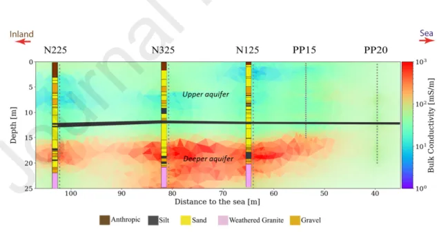
The bulk conductivity (C0) cross-section perpendicular to the coast obtained by CHERT (Figure 5)
shows a very flat SWI wedge located 2 m below a continuous layer of silt identified at 12 m depth. However, the higher spatial resolution obtained with CHERT between wells PP15 and PP20 appear to indicate two different SWI areas, one in the upper part of the aquifer, close to PP20 and another one in the deeper part of the aquifer. These data do not correlate with the EC measured in the piezometers. Indeed, the EC measurements from fully screened piezometers (PP15 and PP20) show relatively constant values of EC between 4 and 12 m depth (Figure 6). Below this depth, there is a general continuous increase in EC towards seawater conductivities that does not correlate with CHERT data. Whereas EC patterns observed in PP15 and PP20 are likely to be artificially affected by the use of fully screened piezometers, further research is required to appropriately understand the difference on conductivity patterns derived from EC measurements in the piezometers and CHERT.
Figure 5. Bulk electrical conductivity model obtained from CHERT data. The anomaly in red, extending throughout the cross-section, 2 m below the continuous layer of silt placed at 12 m depth (in grey), indicates the presence of seawater in the aquifer. The stratigraphic columns of the Argentona site are displayed as a reference for interpretation.
The higher spatial resolution obtained with CHERT allows differentiating two different mixing zones that could be indicative of two different discharging areas: a shallow one with a recirculation cell perhaps influenced by seawater infiltration from waves/storms, and a deeper one discharging away offshore. However, more data is required to verify these hypotheses, as the conductivity measured in the piezometers (Supplementary material, Table 1), shows higher values (i.e. lower resistivity) in the deepest part of the aquifer.
Figure 6. EC profiles recorded at the fully screened piezometer PP20 (Figure 2) in 2015. Fresh and sea water values are marked with a dashed line in the figure for comparison.
The ratio between the bulk electrical conductivity from June and September is a good tool to evaluate the seasonal variation in salinity (Figure 7). Whilst, ratios below 1 (color blue) indicate a decrease of conductivity, ratios above 1 (color red) indicate an increase. The maximum changes occur between 15 and 20 m depth, with a general increase in conductivity mainly in the coarser materials between the piezometers N3 to PP20. This trend is consistent with groundwater level evolution (data not shown) that tend to decrease between 2 and 4 cm between June and September. However, this evolution is not clear in the water electrical
conductivity changes measured in the piezometers (Supplementary material, Table 1). There are changes along the vertical electrical conductivity profiles measured with the EC probe, most significant in June, due to the presence of sediments with different grain size that cause different flow distributions along the 2 m screened intervals of most piezometers. Furthermore, compared with piezometers data, CHERT models shows the extension of the area affected by this increase of conductivity in the sands as well as in the weathered granite.
In the upper part of the aquifer there are no significant variations of conductivity as indicated by data obtained in the piezometers PP15 and PP20 (Supplementary material, Table 1), pointing out that a relatively stable SWI between June and September at shallow depths.
Figure 7. Cross-section of the bulk electrical conductivity (C0) ratio between June and September 2015 CHERT
surveys. The colour scale varies from a decrease to half of the value of C0 compared to June 2015 (blue), to an
increase by two in the value of C0 compared to June 2015 (red). The main change during summer is a twofold
increase in bulk EC observed 2 m below the silt layer at -12 m depth represented in grey. The stratigraphic columns of the Argentona site are displayed as a reference for interpretation.
4.2 Time-lapse induction logging (TLIL)
Time-lapse downhole measurements were carried out in piezometer N320 only and at the onset of the dry season (May 2015). Downhole measurements are repeated every 15 minutes in the
same hole, in a time-lapse mode, and surface conductivity (Cs) and formation factor (F) were
considered constant (Equation 1). Consequently, changes in bulk electrical conductivity are attributed to changes in groundwater conductivity due to changes in pore fluid temperature and/or salinity with time.
Figure 8. a) Downhole Induction logging (IL) profiles of formation electrical conductivity (C0) measured in borehole
N320 (Figure 1) on May 11th, 2015 (profiles IL1, IL2 and IL3) between 3:00 and 3:45 PM, and on May 12th, 2015 at
11:30 AM (profile IL23). (b) Stratigraphic column of N325 (Figure 2) located 1.5 m away from N320 (c) Pore fluid conductivity ratios (∆C0), taking the May 12th, 2015 profile IL23 as reference. Grey shadings across the entire figure
point at levels where high frequency conductivity changes between profiles recorded on May 11th, 2015 were
detected.
We considered that changes in formation conductivity (C0) were directly proportional to changes
measured a month later in the same piezometer (Supplementary materials, Table 1). The maximum C0 values were obtained below 14 m depth, in agreement with piezometers data and
the June 2015 CHERT acquisition/cross-section. In this way, groundwater at the top of the screened interval for N320 showed values in agreement with the conductivity of 13.3 mS/cm measured in this piezometer in June.
When considering C0 changes over short periods of time (10's of minutes), some depth intervals
present significant changes between May 11th and 12th, 2015 (Figure 8a). Changes can be
revealed by calculating pore fluid conductivity ratios (∆C0) of each profile taking the May 12th,
2015 profile (IL23) as reference. Close to the surface (from 3 to 9 m depth), were we can find fresher groundwater, all ratios exhibit a decrease in conductivities overnight, with changes up to 30% (Figure 8c, Pore fluid conductivity ratios (∆C0)). This decrease can be due to a decrease
in groundwater temperature or salinity overnight, or both in the same time period. In the same depth interval, smaller changes of 5 to 10% are noticed between IL3 and IL4 (Figure 8c, orange and green profiles) that is in less than 15 minutes. These smaller changes appear in decimeter-thick intervals (near 5.5 and 6.5 m depth) and point at small changes in groundwater temperature or salinity in a very short time. These high frequency conductivity changes (grey sections in Figure 8) are attributed to the presence of preferential flow pathways with relatively high fluid flow at these depths. It can be noticed that the TLIL method identified small zones of preferential flow that cannot be identified with CHERT.
In the brackish to sea-water saturated region below 9 m depth, very little conductivity changes were registered, in occasions less than 0.5%. These horizons correspond to finer grained materials where fluid flow is troublesome. Between 14.5 and 15.5 m depth, noticeable changes up to 5% are measured over a meter-thick interval. These tiny changes underline the precision of TLIL measurements. Below 16 m depth (Figure 8c), no significant changes in C0 are observed
4.3. Fiber optic distributed temperature sensing (FO-DTS)
Rather than presenting the results as temperature depth profiles, we choose to interpolate the data with a simple linear interpolation perpendicular to the sea to highlight the spatial patterns (Figure 9). Unlike the geophysical techniques, which provide a wider distribution of measures in the subsurface, FO-DTS data concentrates on several vertical lines. Therefore, the uncertainty of the interpolation is larger, and any future qualitative analysis would be better based on the un-processed temperature data (i.e. the vertical temperature depth profiles). However, interpolated plots allow a good qualitative analysed and comparison between the different techniques performed in this study.
The general distribution of temperature follows the same trend as piezometer measurements (Supplementary material, Table 2), with higher temperatures inland and lower closer to the sea (Figure 9). However, all temperatures measured in the piezometers are higher than those measured with DTS. While the maximum temperature in groundwater according to the FO-DTS is below 19.40 °C, several temperature measurements in piezometers are above this value. This pattern is observed in the wells with a 2 m screened interval as well as those completely screened (PP15 and PP20), where the complete cross-section tends to show higher temperature. The higher values measured in the piezometers compared with the distribution observed with the FO-DTS indicates that temperature in piezometers is significantly altered by atmospheric temperature. In contrast, the fiber installed in the annular space of the piezometers, measured temperatures much closer to the expected subsurface temperatures.
The highest influence of the atmospheric temperature is above the first 3 m depth, corresponding to the non-saturated zone. In this regard, the annual thermal oscillation extinction point was estimated to be less than 15 m depth applying the solution proposed by Stauffer et al., (2013) with the local atmospheric temperature in the period May-September
2015 (data not shown). Between June and September, this influence can be reduced to 12 m depth. Considering that neither the vertical nor the horizontal distribution of temperature underground is homogenous, different effects can condition groundwater temperature distribution. However, the small influence of atmospheric temperature on groundwater temperature at shallow depths indicate that groundwater flow in this area is relatively important, which is in accordance with the coarser grain of the materials found in the upper part of the aquifer.
In June (Figure 9a), the temperatures are generally lower than in September, showing more spatial changes in the upper part of the aquifer than at the bottom. It is clear that there are two sources of temperature anomalies relating to the coldest and hottest temperatures of the cross-section. The coldest anomaly located between N325 and N125 is attributed to the local effect of surface recharge from a discontinuous sewerage discharge channel close to the site, as also observed in temperature data from the N4 nest (data not shown) which is located close to this discharge area. The warmest temperature of the cross-section is observed in the inland part of the experimental site (between N225 and N325) highlighting the thermal effect of groundwater flow recharged inland. The coldest temperatures of the cross-section are measured at the deepest part of the aquifer at the bottom of a thick pack of sands below 18 m and close to the weathered granite. Since this is the most affected area by SWI, the coldest temperatures derived from FO-DTS data are related to the intrusion of colder seawater, in contrast with the warmer temperatures observed inland. In this regard, the small areas with the coolest temperatures around at depth of 11 m, close to N125 and PP15, could also be indicating the presence of a shallower saltwater wedge.
Figure 9. Thermal profiles of the June and September field surveys resulting from linear interpolation of data in each borehole. Temperatures above 20 °C are all drawn with the same color. The stratigraphic columns of the Argentona site are displayed as a reference for interpretation. Grey layer indicates a continuous layer of silt that crosses all piezometers
In September (Figure 9b), temperature distribution is similar to June, but with slightly higher values. The non-saturated zone, as well as the deepest part of the cross-section, shows higher temperatures. As in June, the warmest temperatures are located at the innermost and shallow part of the aquifer and the coldest temperatures at the deepest part of the aquifer, closer to the sea. However, there is a slight increase of the coldest temperatures in the deeper part of the aquifer, which could be related to the higher temperatures along the profile due to the dry season, an increase of sea water temperature, or both. In the same way, when considering only
the shallow part of the aquifer, the coldest temperature corresponds to the part of the profile closest to the sea. However, during summer there is an increase in sea water temperature in the shallow depths that does not seem to affect the temperature distribution in the upper part of the aquifer in the closer zone to the sea.
5. Discussion and integration of techniques
The combination of techniques applied in the Argentona site allows describing the behaviour of the system at the beginning and at the end of the dry season. The shallowest part of the aquifer does not show important salinity changes during the studied period. On the other hand, the deepest part of the aquifer shows an increase in salinity over the season, mainly observed in the bottom part of the sedimentary formation. Despite the basement showing a high electrical conductivity, the values measured remain constant during the studied period (i.e. low flow). This lack of dynamism is in agreement with the low transmissivity obtained through short pumping tests (Martínez-Pérez et al. 2018, Internal communication). At borehole scale, induction logging revealed the presence of preferential flow paths at different depths.
Whereas each applied technique provides partial information of the coastal aquifer, the combination of techniques allows obtaining a comprehensive understanding of the characteristics and hydrodynamics of this complex system. CHERT and FO-DTS provide important information at the site scale, whereas TLIL characterizes the system at the meter-scale. With CHERT and FO-DTS data we can differentiate two behaviours in the aquifer. While CHERT identified the main active area of SWI intrusion occurring in the deepest part, FO-DTS does not show important changes between both surveys. However, FO-DTS and TLIL highlighted that the shallowest part of the aquifer is an active system with fresh groundwater flow occurring; a statement that cannot be made by looking only at CHERT.
The active area identified with TLIL in the deepest part of the aquifer at 15 m depth (Figure 8), corresponds to the upper part of the active area identified with CHERT (Figure 7). On the contrary, no significant changes are observed with TLIL below 16 m unlike what was found by CHERT. These differences between both methods could be related to the fact that both are deployed at different spatial and temporal scales. In this way, CHERT could point more to seasonal changes, while TLIL may be related to more instantaneous changes. Whilst we cannot evaluate the capacity of CHERT to identify hourly or daily changes with the data collected, we infer that it would be possible to capture such changes with a proper experimental design that allows to acquire data with a high temporal frequency. More research is needed to understand this issue, increasing the number of points were Co is measured and/or by increasing the
temporal frequency of CHERT profiles.
Despite the high density of piezometers in the field site, and the screening of the piezometer on only 2 m, these techniques provide higher spatial resolution than direct measurements. Furthermore, they can give more representative information of the SWI extent, especially CHERT. In this regard, CHERT data correlates relatively well with water electrical conductivity of most piezometers in the different locations and depths along the study site. However, CHERT provides a 2D representation of the shape and extent of the seawater intrusion and its seasonal variations. This information would be impossible to obtain using only point measurements from piezometers. This is particularly relevant in fully screened piezometers.
Temperature measured with FO-DTS in the annular space of the boreholes (i.e., closer to the aquifer matrix) is lower than temperature measured in the piezometers, pointing out the influence of atmospheric/soil conditions on groundwater measurements from piezometers. The changes in formation electrical conductivity measured with TLIL may indicate preferential flows at a smaller scale than the other techniques, giving information that cannot be obtained and/or approximated with traditional monitoring methods. Only tracer tests in the screened
intervals could generate similar data but with lower spatial and temporal resolution, and at higher costs.
The study site is located in the Mediterranean basin and therefore subjected to a microtidal regime. In other oceanic coastal areas, the effect of tides is more significant and can influence the dynamics of the system. It is expected that in open sea areas the applied methods could improve the characterization of the system. That is particularly relevant for the FO-DTS, as higher tides increase the dynamism of the SWI, increasing the thermal influence of the sea boundary condition on the aquifer. This assumption could explain why the influence of the sea has been found to be minor in this study, despite various studies indicate that temperature can be used as a useful SWI tracer. In the same way, the application of this technique in those areas with important thermal contrast between sea and groundwater temperature could give better results. Finally, the connection to the sea and the thermal properties of the geological materials could limit the application of this technique.
6. Conclusions and future challenges
Different approaches and techniques (direct groundwater measurements from piezometers, CHERT, FO-DTS and TLIL) have been combined for the first time to study a 25-m thick microtidal coastal aquifer during the dry season (before and after summer 2015). CHERT profiles allow a better definition of the shape and distribution of the seawater intrusion, as well as its seasonal changes, than data obtained from point groundwater measurements from piezometers. In this case study, the combination of the different techniques has allowed improving the understanding of the hydrogeological system by: 1) A proper characterization of the extend and shape of the SWI, 2) differentiating two different zones with different dynamics in the deep and upper part of the aquifer and 3) identifying preferential flow paths over different time and spatial intervals. The distribution of the SWI does not follow the typical shape, with main
changes between 15 and 18 m depth. Despite minor changes in salinity measured in the shallower part of the aquifer, data provided by TLIL and FO-DTS indicate that it is an active system.
Although precise characterization of the aquifer was achieved by combining different geophysical techniques, the groundwater discharge process to the coastal sea (i.e. SGD) is still a challenge. Considering the information obtained from the techniques applied, there are two different mixing zones that could be related to two different discharge areas: a shallow recirculation cell closer to the sea, mainly influenced by wave setup and storm effects (in addition to the terrestrial hydraulic gradient), and a deep discharge area, acting at a more seasonal scale, and likely discharging offshore. However, the extension of the discharge of the deep aquifer into the sea is not fully clear. More data are required to fill the blank between the site and the sea, but also inland, to improve the understanding of the system. Yet, a higher temporal and spatial resolution of the already applied techniques will also improve the understanding of the system considering the following:
- Higher temporal resolution of CHERT would allow understanding how mixing is occurring and the origin of salinity in the shallow part of the aquifer (convective zones, wave effect, etc.). At the same time, higher temporal resolution would allow understanding why at the end of the dry season there is a decrease of salinity simultaneously with an increase of salinity in the deeper part of the aquifer.
- TLIL could be applied in more piezometers at the same time to study the changes in conductivity and check whether these changes correspond to preferential flows at decimeter scale. In the same way, using this technique with higher frequency could allow understanding if these potential preferential flow paths respond to to the heterogeneity of the system and/or the recharges/discharges processes occurring at different temporal scales (storms events versus seasonal dynamics).
- FO-DTS has allowed obtaining more information in areas with no TLIL data and/or where the conductivity changes are not significant to obtain representative data with CHERT. Nevertheless, only minor differences between both surveys are measured. Therefore, the potential use of temperature as a tracer using FO-DTS needs to be evaluated for a longer period of time as its distribution is significantly affected by the thermal characteristics of the boundary conditions (atmosphere, recharge inland, sea, etc.) and therefore changing along seasons. In this way, it is important to consider that the boundary conditions tend to change in a similar way along seasons but with some lag and different extreme values.
Although more research is needed, the application of the presented techniques in a well-characterized study area such as the Argentona site has allowed describing the effectiveness of FO-DTS, CHERT and TLIL to characterize coastal areas dynamics. This information has pointed out the potential of these techniques to be applied in other areas. In this way, the best technique to use when characterizing coastal aquifers dynamics will depend on the temporal and spatial resolution required. The importance of fresh water flow in the system can also indicate which methods should be combined and the amount of data that is required. The structure of the aquifer (unconfined/confined vs multilayer aquifer), and the boundary conditions (recharge patterns, thermal contrast between boundaries, etc.) can also condition the combination of techniques to be used. Lastly, studying zones in small basins as the Mediterranean or on the contrary in open ocean conditions, will also influence the approach to apply due to the different dynamics of costal aquifer in both areas. In all cases, the electrical conductivity and temperature data obtained with the CHERT, FO-DTS and TLIL is expected to be more representative than the same data obtained in the piezometers.
Aknowlegments
This work was funded by the projects CGL2013-48869-C2-1-R/2-R and
CGL2016-77122-C2-1-R/2-R of the Spanish Government. We would like to thank SIMMACGL2016-77122-C2-1-R/2-R (Serveis Integrals de
Manteniment del Maresme) and the Consell Comarcal del Maresme in the construction of the
research site. The authors want to thank the support of the Generalitat de Catalunya to MERS
(2018 SGR-1588). This work is contributing to the ICTA ‘Unit of Excellence’ (MinECo,
MDM2015-0552). Part of the funding was provided by the French network of hydrogeological observatories
H+ (hplus/ore/fr/en) and the ANR project EQUIPEX CRITEX (grant ANR-11-EQPX-0011). V
Rodellas acknowledges financial support from the Beatriu de Pinós postdoctoral program of the
Generalitat de Catalunya (2017-BP-00334). M. Diego-Feliu acknowledges the economic support
from the FI-2017 fellowships of the Generalitat de Catalunya autonomous government
(2017FI_B_00365). This project also received funding from the European Union’s Horizon 2020
research and innovation programme under the Marie Sklodowska-Curie Grant Agreement No
722028.
7. References
Anwar, N., Robinson, C., Barry, D.A., 2014. Influence of tides and waves on the fate of nutrients in a nearshore aquifer: Numerical simulations. Adv. Water Resour. 73, 203–213.
https://doi.org/10.1016/J.ADVWATRES.2014.08.015
Badaruddin, S., Werner, A.D., Morgan, L.K., 2015. Water table salinization due to seawater intrusion. Water Resour. Res. 51, 8397–8408. https://doi.org/10.1002/2015WR017098 Bakker, M., Calj, R., Schaars, F., Made, K.-J. van der, Haas, S. de, 2015. An active heat tracer
experiment to determine groundwater velocities using fiber optic cables installed with direct push equipment. Water Resour. Res. 51, 2760–2772.
https://doi.org/10.1002/2014WR016632
Beaujean, J., Nguyen, F., Kemna, A., Antonsson, A., Engesgaard, P., 2017. Calibration of seawater intrusion models: Inverse parameter estimation using surface electrical resistivity tomography and borehole data. Water Resour. Res. 50, 6828-6849 https://doi.org/10.1002/2013WR014020
Bellmunt, F., Marcuello, A., Ledo, J., Queralt, P., 2016. Capability of cross-hole electrical configurations for monitoring rapid plume migration experiments. J. Appl. Geophys. 124, 73–82. https://doi.org/10.1016/J.JAPPGEO.2015.11.010
Bense, V.F., Read, T., Bour, O., Le Borgne, T., Coleman, T., Krause, S., Chalari, A., Mondanos, M., Ciocca, F., Selker, J.S., 2016. Distributed Temperature Sensing as a downhole tool in hydrogeology. Water Resour. Res. 764, 52, 9259–9273.
https://doi.org/10.1002/2016WR018869
Bone, S.E., Charette, M.A., Lamborg, C.H., Gonneea, M.E., 2007. Has submarine groundwater discharge been overlooked as a source of mercury to coastal waters? Environ. Sci. Technol. 41, 3090–3095. https://doi.org/10.1021/es0622453
Briggs, M.A., Buckley, S.F., Bagtzoglou, A.C., Werkerma, D.D. and Lane, J.W., 2016. Actively heated high-resolution fiber-optic-distributed-temperature sensing to quantify
streambed flow dynamics in zones of strong groundwater upwelling. Water Resour. Res. 52, 5179 - 5194. https://doi.org/10.1002/2015WR018219
Brovelli, A., Mao, X., Barry, D.A., 2007. Numerical modeling of tidal influence on density-dependent contaminant transport. Water Resour. Res. 43. W10426.
https://doi.org/10.1029/2006WR005173
Camporese, M., Cassiani, G., Deiana, R., Salandin, P., 2011. Assessment of local hydraulic properties from electrical resistivity tomography monitoring of a three-dimensional
synthetic tracer test experiment. Water Resour. Res. 47. https://doi.org/10.1029/2011WR010528
Cassiani, G., Bruno, V., Villa, A., Fusi, N., Binley, A.M., 2006. A saline trace test monitored via time-lapse surface electrical resistivity tomography. J. Appl. Geophys. 59, 244–259. https://doi.org/10.1016/J.JAPPGEO.2005.10.007
Cerdà-Domènech, M., Rodellas, V., Folch, A., Garcia-Orellana, J., 2017. Constraining the temporal variations of Ra isotopes and Rn in the groundwater end-member: Implications for derived SGD estimates. Sci. Total Environ. 595, 849-857.
.https://doi.org/10.1016/j.scitotenv.2017.03.005
de Franco, R., Biella, G., Tosi, L., Teatini, P., Lozej, A., Chiozzotto, B., Giada, M., Rizzetto, F., Claude, C., Mayer, A., Bassan, V., Gasparetto-Stori, G., 2009. Monitoring the saltwater intrusion by time lapse electrical resistivity tomography: The Chioggia test site (Venice Lagoon, Italy). J. Appl. Geophys. 69, 117–130.
https://doi.org/10.1016/J.JAPPGEO.2009.08.004
Debnath, P., Mukherjee, A., Singh, H.K., Mondal, S., 2015. Delineating seasonal porewater displacement on a tidal flat in the Bay of Bengal by thermal signature: Implications for submarine groundwater discharge. J. Hydrol. 529, 1185–1197.
https://doi.org/10.1016/j.jhydrol.2015.09.029
Denchik, N., Pezard, P.A., Neyens, D., Lofi, J., Gal, F., Girard, J.-F., Levannier, A., 2014. Near-surface CO2 leak detection monitoring from downhole electrical resistivity at the CO2
Field Laboratory, Svelvik Ridge (Norway). Int. J. Greenh. Gas Control 28, 275–282. https://doi.org/10.1016/J.IJGGC.2014.06.033
Dror, I., Amitay, T., Yaron, B., Berkowitz, B., 2003. Salt-pump mechanism for contaminant intrusion into coastal aquifers. Science 80, 950. https://doi.org/10.1126/science.1080075
Garing, C., Luquot, L., Pezard, P.A., Gouze, P., 2013. Geochemical investigations of saltwater intrusion into the coastal carbonate aquifer of Mallorca, Spain. Appl. Geochemistry 39, 1– 10. https://doi.org/10.1016/J.APGEOCHEM.2013.09.011
Giambastiani, B.M.S., Colombani, N., Greggio, N., Antonellini, M., Mastrocicco, M., 2017. Coastal aquifer response to extreme storm events in Emilia-Romagna, Italy. Hydrol. Process. 31, 1613–1621. https://doi.org/10.1002/hyp.11130
Goebel, M., Pidlisecky, A., Knight, R., 2017. Resistivity imaging reveals complex pattern of saltwater intrusion along Monterey coast. J. Hydrol. 551, 746–755.
https://doi.org/10.1016/j.jhydrol.2017.02.037
Günther, T., Rücker, C., Spitzer, K., 2006. Three-dimensional modelling and inversion of dc resistivity data incorporating topography - II. Inversion. Geophys. J. Int. 166, 506–517. https://doi.org/10.1111/j.1365-246X.2006.03011.x
Hausner, M.B., Kryder, L., Klenke, J., Reinke, R., Tyler, S.W., 2016. Interpreting Variations in Groundwater Flows from Repeated Distributed Thermal Perturbation Tests. Groundwater 54, 559–568. https://doi.org/10.1111/gwat.12393
Henderson, R.D., Day-Lewis, F.D., Lane, J.W., Harvey, C.F., Lanbo, L., 2008. Characterizing Submarine Ground-Water Discharge Using Fiber-Optic Distributed Temperature Sensing and Marine Electrical Resistivity. Sageep 1–11. https://doi.org/10.4133/1.2963319 Henderson, R.D., Day-Lewis, F.D., Abarca, E., Harvey, C.F, Karam, H.N., Liu, L., Lane, J.W., Jr.,
2010. Marine electrical resistivity imaging of submarine groundwater discharge:
sensitivity analysis and application in Waquoit Bay, Massachusetts, USA. Hydrogeology J. 18, 173-185. https://doi.org/10.1007/s10040-009-0498-z
Huizer, S., Karaoulis, M.C., Oude Essink, G.H.P., Bierkens, M.F.P., 2017. Monitoring and simulation of salinity changes in response to tide and storm surges in a sandy coastal
aquifer system. Water Resour. Res. 53, 6487–6509. https://doi.org/10.1002/2016WR020339
Kim, G., Kim, J.-S., Hwang, D.-W., 2011. Submarine groundwater discharge from oceanic islands standing in oligotrophic oceans: Implications for global biological production and organic carbon fluxes. Limnol. Oceanogr. 56, 673–682.
https://doi.org/10.4319/lo.2011.56.2.0673
Klepikova, M. V., Le Borgne, T., Bour, O., Gallagher, K., Hochreutener, R., Lavenant, N., 2014. Passive temperature tomography experiments to characterize transmissivity and connectivity of preferential flow paths in fractured media. J. Hydrol. 512, 549–562. https://doi.org/10.1016/j.jhydrol.2014.03.018
Koestel, J., Kemna, A., Javaux, M., Binley, A., Vereecken, H., 2008. Quantitative imaging of solute transport in an unsaturated and undisturbed soil monolith with 3-D ERT and TDR. Water Resour. Res. 44, W12411. https://doi.org/10.1029/2007WR006755
Martínez, M.L., Intralawan, A., Vázquez, G., Pérez-Maqueo, O., Sutton, P., Landgrave, R., 2007. The coasts of our world: Ecological, economic and social importance. Ecol. Econ. 63, 254– 272. https://doi.org/10.1016/j.ecolecon.2006.10.022
Martínez-Perez, L., Marazuela, M.A., Luquot, L., Folch, A., del Val, L., Goyetche, T., Diego-Feliu, M., Ferrer, N., Rodellas, V., Bellmunt, F., Ledo, J., Pool, M., Garcia-Orellana, J., Pezard, P., Saaltink, M., Vazquez-Suñe, E., Carrera, J., 2018. Integrated methodology to characterize hydro-geochemical properties in an alluvial coastal aquifer affected by seawater intrusion (SWI) and submarine groundwater discharge (SGD). 25th Saltwater Intrusion Meeting. Gdansk, Poland.
Michael, H.A., Mulligan, A.E., Harvey, C.F., 2005. Seasonal oscillations in water exchange between aquifers and the coastal ocean. Nature 436, 1145–1148.
https://doi.org/10.1038/nature03935
Michael, H.A., Post, V.E.A., Wilson, A.M., Werner, A.D., 2017. Science, society, and the coastal groundwater squeeze. Water Resour. Res. 53, 2610–2617.
https://doi.org/10.1002/2017WR020851
Moore, W.S., 1999. The subterranean estuary: a reaction zone of ground water and sea water. Mar. Chem. 65, 111–125. https://doi.org/10.1016/S0304-4203(99)00014-6
Moore, W.S., 2010. The Effect of Submarine Groundwater Discharge on the Ocean. Ann. Rev. Mar. Sci. 2, 59–88. https://doi.org/10.1146/annurev-marine-120308-081019
Morrow, F.J., Ingham, M.R., McConchie, J.A., 2010. Monitoring of tidal influences on the saline interface using resistivity traversing and cross-borehole resistivity tomography. J. Hydrol. 389, 69–77. https://doi.org/10.1016/J.JHYDROL.2010.05.022
Müller, K., Vanderborght, J., Englert, A., Kemna, A., Huisman, J.A., Rings, J., Vereecken, H., 2010. Imaging and characterization of solute transport during two tracer tests in a shallow aquifer using electrical resistivity tomography and multilevel groundwater samplers. Water Resour. Res. 46, W03502. https://doi.org/10.1029/2008WR007595 Nguyen, F., Kemna, A., Antonsson, A., Engesgaard, P., Kuras, O., Ogilvy, R., Gisbert, J., Jorreto,
S., Pulido-Bosch, A., 2009. Characterization of seawater intrusion using 2D electrical imaging. Near Surf. Geophys. 7, 377-390. https://doi.org/10.3997/1873-0604.2009025 O’Connor, A.E., Luek, J.L., McIntosh, H., Beck, A.J., 2015. Geochemistry of redox-sensitive trace
elements in a shallow subterranean estuary. Mar. Chem. 172, 70–81. https://doi.org/10.1016/J.MARCHEM.2015.03.001
Palacios, A., Ledo, J. J., Linde, N., Luquot, L., Bellmunt, F., Folch, A., Marcuello, A., Queralt, P., Pezard, P. A., Martínez, L., Bosch, D., and Carrera, J., 2020. Time-lapse cross-hole
Mediterranean aquifer, Hydrol. Earth Syst. Sci. Discuss., https://doi.org/10.5194/hess-2019-408, accepted.
Pauw, P.S., Groen, J., Groen, M.M. A., van der Made, K.J., Stuyfzand, P.J., Post, V.E. A., 2017. Groundwater salinity patterns along the coast of the Western Netherlands and the application of cone penetration tests. J. Hydrol. 551, 756–767.
https://doi.org/10.1016/j.jhydrol.2017.04.021
Perri, M.T., Cassiani, G., Gervasio, I., Deiana, R., Binley, A., 2012. A saline tracer test monitored via both surface and cross-borehole electrical resistivity tomography: Comparison of time-lapse results. J. Appl. Geophys. 79, 6–16.
https://doi.org/10.1016/j.jappgeo.2011.12.011
Pezard, P.A., Abdoulghafour, H., Denchik, N., Perroud, H., Lofi, J., Brondolo, F., Henry, G., Neyens, D., 2015. On Baseline Determination and Gas Saturation Derivation from Downhole Electrical Monitoring of Shallow Biogenic Gas Production. Energy Procedia 76, 555–564. https://doi.org/10.1016/j.egypro.2015.07.910
Re, V., Sacchi, E., Mas-Pla, J., Menció, A., El Amrani, N., 2014. Identifying the effects of human pressure on groundwater quality to support water management strategies in coastal regions: A multi-tracer and statistical approach (Bou-Areg region, Morocco). Sci. Total Environ. 500–501, 211–223. https://doi.org/10.1016/j.scitotenv.2014.08.115
Rodellas, V., Garcia-Orellana, J., Masqué, P., Feldman, M., Weinstein, Y., 2015. Submarine groundwater discharge as a major source of nutrients to the Mediterranean Sea. Proc. Natl. Acad. Sci. U. S. A. 112, 3926–30. https://doi.org/10.1073/pnas.1419049112 Rosenberry, D.O., Briggs, M.A., Delin, G. and Hare, D.K. 2016. Combined use of thermal
methods and seepage meters to efficiently locate, quantify, and monitor focused groundwater discharge to a sand-bed stream. Water Resour. Res. 52, 4486-4503.
https://doi.org/10.1002/2016WR018808
Rücker, C., Günther, T., Wagner, F.M., 2017. pyGIMLi : An open-source library for modelling and inversion in geophysics. Comput. Geosci. 109, 106–123.
https://doi.org/10.1016/j.cageo.2017.07.011
Rufí-Salís, M., Garcia-Orellana, J., Cantero, G., Castillo, J., Hierro, A., Rieradevall, J., Bach, J., 2019. Influence of land use changes on submarine groundwater discharge. Environ. Res. Commun. 1, 031005. https://doi.org/10.1088/2515-7620/ab1695
Santos, I.R., Burnett, W.C., Dittmar, T., Suryaputra, I.G.N.A., Chanton, J., 2009. Tidal pumping drives nutrient and dissolved organic matter dynamics in a Gulf of Mexico subterranean estuary. Geochim. Cosmochim. Acta 73, 1325–1339.
https://doi.org/10.1016/J.GCA.2008.11.029
Selker, J.S., Thévenaz, L., Huwald, H., Mallet, A., Luxemburg, W., Van De Giesen, N., Stejskal, M., Zeman, J., Westhoff, M., Parlange, M.B., 2006. Distributed fiber-optic temperature sensing for hydrologic systems. Water Resour. Res. 42, W12202.
https://doi.org/10.1029/2006WR005326
Simon, N., Bour, O., Lavenant, N., Porel, G., Nauleau, B., Pouladi, B., Longuevergne, L, 2020. A comparison of different methods to estimate the effective spatial resolution of FO-DTS measurements achieved during sandbox experiments, Sensors 20, 570.
doi:10.3390/s20020570)
Singha, K., Day-Lewis, F.D., Johnson, T., Slater, L.D., 2015. Advances in interpretation of subsurface processes with time-lapse electrical imaging. Hydrol. Process. 29, 1549–1576. https://doi.org/10.1002/hyp.10280
Spiteri, C., Slomp, C.P., Charette, M.A., Tuncay, K., Meile, C., 2008. Flow and nutrient dynamics in a subterranean estuary (Waquoit Bay, MA, USA): Field data and reactive transport
modeling. Geochim. Cosmochim. Acta 72, 3398–3412. https://doi.org/10.1016/J.GCA.2008.04.027
Stauffer, F., Bayer, P., Blum, P., Giraldo, N.M., Kinzelbach, W., Bayer, P., Blum, P., Giraldo, N.M., Kinzelbach, W., 2013. Thermal Use of Shallow Groundwater. CRC Press. https://doi.org/10.1201/b16239
Taniguchi, M., 2000. Evaluations of the saltwater-groundwater interface from borehole temperature in a coastal region. Geophys. Res. Lett. 27, 713–716.
https://doi.org/10.1029/1999GL002366
Trezzi, G., Garcia-Orellana, J., Rodellas, V., Masqué, P., Garcia-Solsona, E., Andersson, P.S., 2017. Assessing the role of submarine groundwater discharge as a source of Sr to the Mediterranean Sea. Geochim. Cosmochim. Acta 200, 42–54.
https://doi.org/10.1016/J.GCA.2016.12.005
Tyler, S.W., Selker, J.S., Hausner, M.B., Hatch, C.E., Torgersen, T., Thodal, C.E., Schladow, S.G., 2009. Environmental temperature sensing using Raman spectra DTS fiber-optic methods. Water Resour. Res. 45, W00D23. https://doi.org/10.1029/2008WR007052
van de Giesen, N., Steele-Dunne, S.C., Jansen, J., Hoes, O., Hausner, M.B., Tyler, S., Selker, J., 2012. Double-ended calibration of fiber-optic Raman spectra distributed temperature sensing data. Sensors 12, 5471–5485. https://doi.org/10.3390/s120505471
Waxman, M.H , Smits, L.M., 1968. 1863-A - Electrical Conductivities in Oil-Bearing Shaly Sands. Soc. Pet. Eng. J. 8, 107–122.
Werner, A.D., Bakker, M., Post, V.E.A., Vandenbohede, A., Lu, C., Ataie-Ashtiani, B., Simmons, C.T., Barry, D.A., 2013. Seawater intrusion processes, investigation and management: Recent advances and future challenges. Adv. Water Resour. 51, 3–26.