Global distribution of tropospheric ozone from satellite measurements using the empirically corrected tropospheric ozone residual technique: Identification of the regional aspects of air pollution

HAL Id: hal-00300972

https://hal.archives-ouvertes.fr/hal-00300972

HAL is a multi-disciplinary open access

archive for the deposit and dissemination of sci-entific research documents, whether they are pub-lished or not. The documents may come from teaching and research institutions in France or abroad, or from public or private research centers.

L’archive ouverte pluridisciplinaire HAL, est destinée au dépôt et à la diffusion de documents scientifiques de niveau recherche, publiés ou non, émanant des établissements d’enseignement et de recherche français ou étrangers, des laboratoires publics ou privés.

Global distribution of tropospheric ozone from satellite

measurements using the empirically corrected

tropospheric ozone residual technique: Identification of

the regional aspects of air pollution

J. Fishman, A. E. Wozniak, J. K. Creilson

To cite this version:

J. Fishman, A. E. Wozniak, J. K. Creilson. Global distribution of tropospheric ozone from satellite measurements using the empirically corrected tropospheric ozone residual technique: Identification of the regional aspects of air pollution. Atmospheric Chemistry and Physics Discussions, European Geosciences Union, 2003, 3 (2), pp.1453-1476. �hal-00300972�

ACPD

Print Version Interactive Discussion

c

EGU 2003

Atmos. Chem. Phys. Discuss., 3, 1453–1476, 2003 www.atmos-chem-phys.org/acpd/3/1453/

c

European Geosciences Union 2003

Atmospheric Chemistry and Physics Discussions

Global distribution of tropospheric ozone

from satellite measurements using the

empirically corrected tropospheric ozone

residual technique: Identification of the

regional aspects of air pollution

J. Fishman1, A. E. Wozniak1, 2, 3, and J. K. Creilson1, 2

1

Atmospheric Sciences Research, NASA Langley Research Center, Hampton, Virginia, USA 2

Science Applications International Corporation (SAIC), Hampton, Virginia, USA 3

Currently at Department of Meteorology, University of Maryland, College Park, Maryland, USA

Received: 30 January 2003 – Accepted: 12 March 2003 – Published: 17 March 2003 Correspondence to: J. Fishman ([email protected])

ACPD

Print Version Interactive Discussion

c

EGU 2003

Abstract

Using coincident observations of total ozone from the Total Ozone Mapping Spectrom-eter (TOMS) and stratospheric ozone profiles from the Solar Backscattered Ultraviolet (SBUV) instruments, detailed maps of tropospheric ozone have been derived on a daily basis over a time period spanning more than two decades. The resultant climatological

5

seasonal depictions of the tropospheric ozone residual (TOR) show much more detail than an earlier analysis that had used coincident TOMS and Stratospheric Aerosol and Gas Experiment (SAGE) ozone profiles, although there are many similarities between the TOMS/SAGE TOR and the TOMS/SBUV TOR climatologies. In particular, both TOR seasonal depictions show large enhancements in the southern tropics and

sub-10

tropics in austral spring and at northern temperate latitudes during the summer. The much greater detail in this new data set clearly defines the regional aspect of tropo-spheric ozone pollution in northeastern India, eastern United States, eastern China, and west and southern Africa. Being able to define monthly climatologies for each year of the data record provides enough temporal resolution to illustrate significant

interan-15

nual variability in some of these regions.

1. Introduction

Over the past several years, a number of studies have used information from the Total Ozone Mapping Spectrometer (TOMS) instrument to glean insight into the distribution of tropospheric ozone and the processes that influence its budget (e.g. Fishman et

20

al., 1990; Kim and Newchurch, 1996; 1998; Hudson and Thompson, 1998; Ziemke et al., 1998; 2000; Fishman and Balok, 1999; Thompson et al., 2003). The primary challenge in each of these studies is the separation of the relatively small tropospheric component, generally 5 to 15%, from the total column and then validating the resultant product against existing data sets, usually derived from ozonesonde measurements.

25

ACPD

Print Version Interactive Discussion

c

EGU 2003

and the derived measurements have generally shown good agreement with available validation data sets.

In the current study, we have taken a different approach using as many TOMS mea-surements as possible to derive a tropospheric product. In simplest terms, we con-struct a daily global distribution of the stratospheric component of the total ozone field

5

which should contain only large-scale structure. Next, we use gridded TOMS data at a resolution of 1◦ latitude by 1.25◦longitude to examine a tropospheric product with equivalent resolution. The stratospheric column ozone (SCO) is derived from measure-ments from Solar Backscattered Ultraviolet (SBUV) instrumeasure-ments because they provide the best spatial resolution with enough frequency that relatively good global coverage

10

can be obtained. In the tropics, the subtropics most of the time, and at middle latitudes during the summer and autumn seasons, the distribution of ozone in the stratosphere is invariant enough that observations over five days are generally representative of an average distribution over that 5-day period. Using this methodology, we have produced daily tropospheric ozone residual (TOR) maps between 50◦N and 50◦S from 1979 to

15

2000. A gap exists in this dataset as no TOMS satellite operated between May 1993 and July 1996 and the aerosol index needed for one of the corrections we apply is not available between August 1996 and July 1997.

In an earlier study, Fishman et al. (1990) presented the first climatology of tropo-spheric ozone derived from the TOR technique using the difference between TOMS

20

total ozone and the SCO by subtracting the SCO determined from SAGE (Strato-spheric Aerosol and Gas Experiment) and SAGE II measurements. The relatively infrequent SAGE profiles (normally ∼30 per day) allowed only for the calculation of climatological seasonal (Fishman et al., 1990) or bimonthly (Fishman et al., 1991) dis-tributions. From these studies, enhanced TOR values were found during the Northern

25

Hemisphere (NH) summers and over the tropical South Atlantic Ocean during austral spring. Although there are many similarities between the climatological TOMS/SAGE TOR and the TOMS/SBUV TOR, there are likewise some important differences that come to the fore because the data set available using the current methodology is much

ACPD

Print Version Interactive Discussion

c

EGU 2003

richer. Some of the more interesting regions include northeastern India, eastern United States, eastern China, and west and southern Africa.

As examples of the kinds of studies that can be performed with this new data set, we show that the high spatial resolution of the data can provide new insights into the vertical distribution of ozone over relatively pristine regions where altitude variations

5

are easily quantified (Jiang and Yung, 1996; Kim and Newchurch, 1998; Newchurch et al., 2001). We also demonstrate how the TOR relates to the observed distribution of ozone at the surface during an air pollution episode. Lastly, we show how these data correlate to the population distribution over densely populated areas in India and China.

10

For the most part, TOMS total ozone data (http://toms.gsfc.nasa.gov/ozone/ozone.

html) have primarily been used for global- or quasi-hemispheric-scale studies. The primary purpose of this paper is to demonstrate the regional utility of a new global tro-pospheric ozone database (http://asd-www.larc.nasa.gov/TOR/data.html) derived from the total ozone archive. The examples we present illustrate only a small fraction of

15

studies that can be conducted in the forthcoming years by the scientific community as this data set is utilized.

2. Data

2.1. TOMS total ozone measurements

TOMS total ozone measurements have been available from several satellites since

20

November 1978 (seehttp://toms.gsfc.nasa.gov). Nimbus-7 operated from November 1978 through April 1993; the Earth Probe satellite operated at a relatively low orbit of 540 km and provided higher spatial resolution from July 1996 through December 1997 and then was boosted to a higher orbit of 740 km to obtain complete global coverage. For the current study, Nimbus-7 TOMS data from 1979 through 1993 and Earth Probe

25

ACPD

Print Version Interactive Discussion

c

EGU 2003

Earth Probe have been used in this study to take advantage of the availability of the aerosol index information that is part of the correction we apply to the measurements (Torres and Bhartia, 1999). In early 2001, it was discovered that the TOMS aboard the Earth Probe satellite was experiencing instrument problems and the quality of the total ozone measurements had degraded.

5

Known data anomalies in the total ozone measurements include a significant cross track bias and, unrelated to the instrument problems, the presence of tropospheric aerosols. A Fast Fourier Transform (FFT) routine is applied to the daily gridded TOMS fields to reduce the cross track bias that appears in the data fields as a wave number 14 due to orbital equator crossings. The presence of tropospheric aerosols is determined

10

by the aerosol index data fields and is corrected in the total ozone measurements using the method described by Torres and Bhartia (1999). Summaries of the TOMS instrumental and operational characteristics and ozone data products can be found in Heath et al. (1975) and McPeters et al. (1993; 1996).

2.2. SBUV ozone profiles and the empirical correction

15

Vertical ozone profiles, as well as total ozone measurements, have been derived from measurements made by the backscattered ultraviolet technique since 1970 when the BUV instrument was launched on Nimbus-4 (Heath et al., 1975). A modified ver-sion of that instrument, the SBUV, was launched in October 1978 on the Nimbus-7 spacecraft by NASA and was operational until June 1990 (see http://code916.

20

gsfc.nasa.gov/Public/Space based/sbuv/sbuv.html). Several subsequent launches of a second generation SBUV instrument, the SBUV/2, have been made by the Na-tional Oceanic and Atmospheric Administration (NOAA) on the NOAA-9, NOAA-11, and NOAA-14 satellites launched in 1984, 1988, and 1994, respectively (see http:

//orbit35i.nesdis.noaa.gov/crad/sit/ozone/.

25

The SBUV and SBUV/2 instruments rely on BUV radiance measurements at 12 wavelengths to derive total ozone and vertical ozone profiles. The nadir-looking SBUV instruments complete 14 orbits per day, with a revisit time of approximately 5 days. In

ACPD

Print Version Interactive Discussion

c

EGU 2003

this study we use data records from the 1979 through 1990 SBUV archive and from the 1989 through 2000 SBUV/2 archive. The ozone profile data are archived as 12 Umkher layer amounts in Dobson Units (DU) as seen in Fishman and Balok (1999). The SBUV data were processed by using the Version 6.0 algorithm; SBUV/2 data were processed with a Version 6.1 algorithm to implement a calibration correction specific

5

to the NOAA- 11 SBUV/2 instrument. A description of the Version 6 processing algo-rithm can be found in Bhartia et al. (1996). SBUV and SBUV/2 data sets are available from the NOAA National Environmental Satellite, Data, and Information Service (see

http://orbit-net.nesdis.noaa.gov/crad/sit/ozone). For convenience, references made in this study to the SBUV data set apply to the combined SBUV and SBUV/2 data sets.

10

The integrated amount of ozone in the stratosphere is determined from SBUV pro-files integrated from the tropopause to the top of the atmosphere. Before integration above the tropopause, each SBUV profile is empirically corrected so that the amount of ozone below the tropopause is set equal to the monthly climatological amount deter-mined from the Logan (1999) analysis. This quantity is then subtracted from the SBUV

15

total ozone column to derive the stratospheric component (Fishman and Balok, 1999). That value (i.e. the integrated ozone amount above the tropopause derived from the SBUV measurement) is then used as input to derive a stratospheric ozone field using other such measurements over a five-day period to determine the field for the central day. That quantity is then subtracted from the concurrent TOMS total ozone amount to

20

calculate the TOR for this study. Tropopause height information for the current study uses gridded (2.5◦ latitude by 2.5◦ longitude) analyses provided by the National Cen-ters for Environmental Prediction (NCEP). These analyses are produced every 6 h and the value closest to the time of the SBUV observation is used in the current study.

For the discussion presented in the following sections, we present monthly maps that

25

have been derived from the TOR distribution calculated daily and then averaged over the month. Thus, each 1◦ latitude by 1.25◦longitude pixel shown in each seasonal cli-matology is an average of ∼1600 points (∼90 days × ∼18 years). For comparison, the seasonal climatologies described in Fishman et al. (1990) and Fishman and Brackett

ACPD

Print Version Interactive Discussion

c

EGU 2003

(1997) were derived by binning the individual TOR values derived from TOMS/SAGE into 5◦ latitude by 10◦ longitude boxes over ∼7 years of observations; the result was ∼13 data points per each box and each box consisted of an area 40 times the resolu-tion of the present study. From such a data density, more than half the 1◦ latitude by 1.25◦ longitude boxes would contain no data.

5

3. Results

3.1. Climatological distribution

A considerable effort has been ongoing to ensure consistency in the use of different satellite instruments to measure ozone (WMO, 1998). As different versions of satel-lite data sets are released, retrieved total ozone amounts are modified to take into

10

account certain measurement artifacts that may not have been identified previously. Depending on what release of the satellite data set is used, comparisons with com-puted TOR values have been found to vary by as much as ∼5 DU (Fishman and Brackett, 1997). Previous studies (e.g. Fishman et al., 1990; Hudson and Thomp-son, 1998; Ziemke et al., 1998; 2000; Fishman and Balok, 1999; Thompson et al.,

15

2003) show good agreement between satellite-derived ozone amounts and integrated ozone derived from ozonesonde measurements. Globally averaged, the TOR value in this study is 31.5 DU. For comparison, the average of the TOMS/SAGE TOR was 32.7 DU in Fishman et al. (1990) and 27.5 DU in Fishman and Brackett (1997), using Version 5 (modified to approximate Version 6) and Version 7 of the TOMS data archive

20

releases, respectively. The current study uses a preliminary Version 8 release of the TOMS archive (see discussion in Sect. 2.1; tentative public release date for Version 8 is 2003).

As part of the current study, we compared the stratospheric column ozone amounts using SAGE with the empirically corrected SBUV profiles generated in this study. Using

25

ACPD

Print Version Interactive Discussion

c

EGU 2003

value of 29.9 DU was derived, or ∼9% higher than the TOR when compared with the TOMS/SAGE TOR values when identical sets of TOMS data were used.

The TOMS/SAGE TOR distribution (Fishman et al., 1990) highlighted a number of significant differences between the seasons and between the two hemispheres. One of the most important findings was that the NH summer shows extensive pollution

5

throughout the middle latitudes. The highest regions appeared to be nonspecific plumes downwind of North America, Europe and Asia. Lowest concentrations were observed over the western tropical Pacific.

In the present TOMS/SBUV seasonal depictions shown in Fig. 1, the regional as-pects of these enhancements are significantly better resolved than in the analyses

10

derived using TOMS and SAGE. In the June–July–August (JJA) NH summertime de-piction, for example, highest TOR values are located throughout the eastern United States and throughout eastern Asia. Prominent high values are also seen emanat-ing off the west coast of the United States as well as along the Ganges River Valley in northeastern India. Perhaps the largest difference between the TOMS/SAGE and

15

TOMS/SBUV TOR distributions is what is observed over eastern Asia.

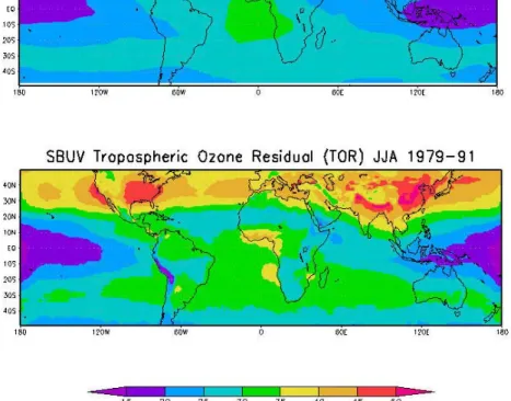
Figure 2 shows for comparison the NH summer distribution for the two data sets us-ing only observations from 1979 through 1991 to capture the same period of measure-ments described in Fishman and Brackett (1997). Considerable detail is now seen over northern India, as well as over central and eastern China, revealing distinct regions of

20

pollution in an area that showed only relatively slightly enhanced levels of TOR in the TOMS/SAGE depiction. In fact, the original TOMS/SAGE TOR over northwest India showed a relative minimum, which was interpreted to be associated with the relatively higher elevations and lack of population in the Tibetan Plateau. The greater detail in the present analysis shows a better-defined, relatively small region of low ozone over

25

the higher elevations. However, just south of that region in the Ganges River Valley, extending west of Delhi and eastward through Bangladesh and northern Burma, much higher values of ozone are observed. High values are now seen throughout central and eastern China.

ACPD

Print Version Interactive Discussion

c

EGU 2003

In the TOMS/SAGE depiction in Fig. 2, the highest TOR values come from the north-ern reaches of the depiction off the east coast of Asia, whereas this region now shows less of an enhancement although a plume downwind of Asia is still evident. The present analysis shows higher values over the landmasses of both the eastern United States and eastern Asia, whereas the older TOMS/SAGE analysis suggested

some-5

what larger concentrations downwind of these continents rather than over the pollution source regions. Whereas the older analysis indicated high values over all of Europe (>45 DU), the current analysis shows lower values (35 to 45 DU) over Europe relative to Asia and the United States.

During the same season, another interesting enhancement is found over the south

10

coast of West Africa. In the TOMS/SAGE depiction, a generally elevated region was seen over the Atlantic Ocean. In the current TOMS/SBUV analysis, this region of enhancement is now much better defined over the coastal landmass of the countries of Liberia, Ivory Coast, Ghana, Togo, Benin, and Nigeria where population density is relatively high. Just north of these elevated regions, considerably lower concentrations

15

(∼25 DU) are found over the Sahara Desert. However, the higher land values seen in this area are opposite the land-sea difference observed over most of northern Africa and the subtropical North Atlantic Ocean and the Mediterranean Sea. Over these ocean areas, the TOR values are higher. Such an artifact has been noted as TOMS “GHOST” (global hidden ozone structures from TOMS) values and has been noted

20

by Cuevas et al. (2001). Some evidence of GHOST is also seen off the west coast of Namibia, a feature clearly observed in the TOMS data shown in Fishman et al. (1990), which used version 5 of the TOMS archive. Most of this artifact was removed in Version 7 (McPeters et al., 1996) when a better cloud algorithm was used to add column ozone amounts in regions where stratus clouds were the dominant cloud type

25

present. The ozone maximum over the South Atlantic off the west coast of Namibia and Angola was shown to be a result of the pollution flowing in the easterlies off of western Africa in combination with the long-range transport from Brazil being carried across the Atlantic after convection elevated the precursors to ozone formation from

ACPD

Print Version Interactive Discussion

c

EGU 2003

biomass burning (Fishman et al., 1996). When viewed from the satellite perspective, the higher values were a result of the addition of the two ozone sources being integrated to produce one sustained region of elevated ozone.

In their discussion of GHOST effects, Cuevas et al. (2001) presented only climato-logical data for the month of July. Because of the seasonality of regional pollution at

5

northern temperate latitudes, sharp delineation along the California coast is a maxi-mum during this time of the year, whereas our TOR analyses show that the land-sea contrast off the coast of Namibia is most enhanced during the biomass burning season of September–October. In TRACE-A, it was shown that the ozone precursors sit off the Namibian west coast and photochemically generate ozone (Fishman et al., 1996),

10

which leads to the September–October–November (SON) depiction in Fig. 1 but ap-pears to a lesser extent in the JJA depiction. It would be interesting to see if the GHOST effect exhibits a similar seasonality in this region. Determination of how much land-sea difference observed in TOMS is caused by tropospheric ozone and how much is an artifact of the retrieval process needs to be examined in future studies.

15

In the SON depiction in Fig. 1, higher values are still seen over the Liberia-to-Nigeria coast and are distinctly separated from the ozone maximum off the Namibian coast. In addition to the broad general maximum observed over the South Atlantic, relatively higher values are also found over the interior of the South American continent and a distinct plume even seems to be emanating from the highly urban Sao Paulo-Rio

20

de Janeiro region. In contrast, there is a well-defined deficit of ozone over the Sahara Desert with the highlands of the desert (northern Chad and northern Niger/southern Al-geria) clearly seen in the SON depiction as well as in the December–January–February (DJF) analysis. The higher terrain of the southwestern Arabian Peninsula is coincident with lower TOR values in this region. Another region of interesting difference is the very

25

low values of TOR over western South America defining in much better detail the loca-tion of the Andes Mountains. This feature is most noticeable in the March–April–May (MAM) and JJA depictions.

ACPD

Print Version Interactive Discussion

c

EGU 2003

southern subtropics relative to what was observed in the TOMS/SAGE depiction, even though both show distinct enhancements over the southern Indian Ocean stretching to Australia (Fishman et al., 1991). Downwind of southern Africa (i.e. to the east), the transport of pollutants off the coast of South Africa and Madagascar appears to be better defined. A relatively small plume appears to originate from Australia.

5

In the Northern Hemisphere, some intriguing enhancements are seen that were not previously observed. Over the southern United States, there is a region of enhance-ment over Texas and Louisiana that did not show up in the TOMS/SAGE TOR. There also seems to be an enhanced region off the California coast, a finding consistent with the modeling study of Stohl et al. (2002), who calculate highest CO concentrations in

10

the eastern Pacific as a result of anthropogenic emissions and subsequent transport from eastern Asia into this region during this time of the year. Higher amounts of ozone are seen in the extreme eastern North Atlantic just south of the Strait of Gibraltar, which is likewise a GHOST region noted by Cuevas et al. (2001).

In the NH spring months, the most pronounced pollution feature is observable over

15

northeastern India and central China. A plume of elevated ozone across the North At-lantic is also present. At this time of the year an enhancement over west central Africa (Congo, Democratic Republic of the Congo (formerly Zaire), and Gabon) is apparent. Depending on the year, somewhat higher values are also seen over northern Brazil. The very low values over the Andes are well defined in this depiction.

20

3.2. Regional scale validation

Fishman et al. (1990) performed a detailed comparison of the TOR with climatological ozonesonde measurements at a number of sites with the conclusion that the satel-lite method captured the absolute amount, seasonality, and interhemispheric gradient reasonably well. Subsequent validation studies comparing against ozonesondes

like-25

wise conclude that the monthly or seasonally averaged amount of tropospheric ozone can be determined to an accuracy of better than 20% (e.g. Kim and Newchurch, 1996; 1998; Fishman and Brackett, 1997; Ziemke et al, 1998; Thompson and Hudson, 1999);

ACPD

Print Version Interactive Discussion

c

EGU 2003

such agreement is not surprising because all these studies use the same TOMS mea-surements as the starting point to derive the tropospheric component. The data used for comparison in this study use the combined 16-year Nimbus-7 and NOAA-11 ozone profile data set with nearly 3000 ozonesonde measurements from 11 stations. SBUV profiles were required to be within a 5◦-latitude by 5◦-longitude box around the station

5

location and on the same day as the sounding. The average differences between the empirically corrected TOMS/SBUV TOR and corresponding tropospheric ozone inte-gral constructed from ozonesonde measurements is 4.0 DU, or ∼13%, again compa-rable with all the previous studies cited above.

However, the real strength from the technique presented here is its ability to extract

10

meaningful ozone distributions on a considerably smaller scale than has previously been investigated. Kim and Newchurch (1996; 1998) have presented interesting stud-ies over South America and Indonesia examining seasonality and trends over a few specific regions, but the large database presented herein lends itself to regional stud-ies nearly anywhere in the world. One example of this richness is detailed in the

depic-15

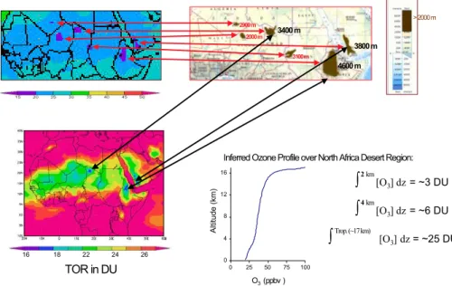
tions shown Fig. 3. The upper left panel is an enlargement of the December-February climatology shown in Fig. 1. This enlargement over northern Africa details the lower values described in the preceding section and compares the location of these lower values with an elevation map of this region shown on the right. At this time of year, locally generated pollution should be minimal and we assume that any regional

varia-20

tions are not a result of local sources. Higher elevations where the altitude is >2000 m are shown in a darker shade of brown. The lower left panel is the same data set in the upper left panel but with a much smaller range of colors (10 DU vs. 50 DU) that bring out additional detail. In the lower left panel, TOR values <18 DU are shown in dark blue and correspond to the higher elevated areas in northern Africa ranging between

25

3400 and 4600 m. Thus, if we assume that the ozone concentration is uniform over the Sahara Desert because there are no inherent sources of pollution, especially dur-ing these photochemically inactive months, the followdur-ing information can be inferred in the lowlands on the fringes of this desert area: A typical TOR value is ∼25 DU;

ACPD

Print Version Interactive Discussion

c

EGU 2003

∼6 DU is below ∼4000 m; and 2 to 3 DU is below ∼2000 m. Unfortunately, there are no ozonesonde measurements in this region, but some measurements at similar latitudes (in India and Hawaii) at the same time of the year suggest that the inferred profile in the lower right portion of the figure is reasonable. This inferred profile could serve as important validation of how sensitive backscatter techniques capture ozone amounts

5

in the lower parts of the atmosphere (Newchurch et al., 2001).

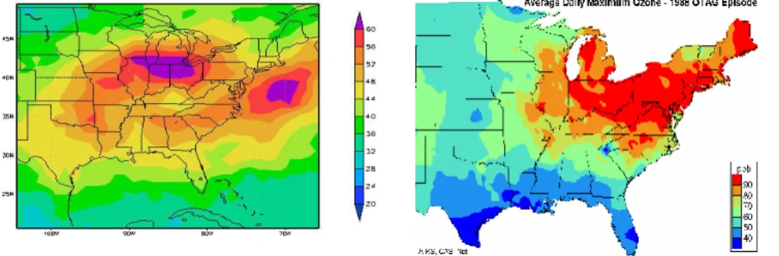
Fishman and Balok (1999) show how the evolution of a regional scale air pollution episode can be inferred from daily TOR maps used in conjunction with meteorological and satellite observations. The relationship between surface ozone concentration and TOR is one that requires considerably more study, but the data sets shown in Fig. 4

10

definitely confirm the strong influence of one upon the other. Fishman et al. (1990) show that both 500 hPa ozone concentrations and TOR values peak during the sum-mer over Wallops Island with values of ∼70 ppb and 45 DU, respectively. Obviously, the shape of the ozone profile is critical for determining how much integrated ozone is in the tropospheric column, but TOR amounts of ∼55 DU (as generally observed over the

15

eastern United States in Fig. 4) and average concentrations of ∼85 ppbv that become well mixed throughout a considerable portion of the lower tropospheric would be con-sistent with the relationship found in the Wallops Island ozonesonde data base. Analo-gously, examining the difference between the areas on either side of the Appalachians with the integrated amount of ozone in the mountains, a deficit of ∼8 DU is observed.

20

With an altitude difference of 1 km between the mountains and the surrounding terrain, an average concentration of ∼90 ppbv would be calculated, again consistent with the observed maximum concentrations measured at the surface.

Both highest surface and TOR values extend along the northern Midwestern indus-trial states from Illinois to western Pennsylvania in the east. The TOR is also elevated

25

off the east coast where there are no surface observations; Fishman and Balok (1999) determined that this offshore reservoir of ozone was likely responsible for the subse-quent episode that formed over the southern United States. It should be noted that the surface depiction shown in this analysis was derived from data from more than 500

ACPD

Print Version Interactive Discussion

c

EGU 2003

EPA monitoring stations in the eastern United States. Nowhere else in the world does there exist such a dense ozone monitoring network over such a large area. Without such a dense data network on this scale, validation studies at only a few sites may incorrectly be assumed to be representative of a larger region, when, in fact, such sites can also be controlled by local features, such as local circulation effects and the

prox-5

imity of nearby sources that result in local measurements being highly dependent on prevailing wind direction.

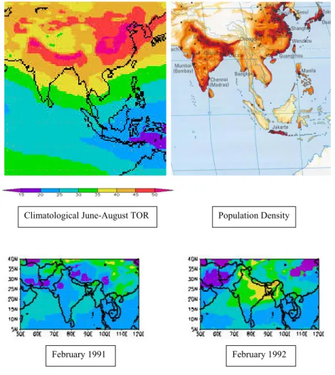
Figure 5 shows for comparison the summertime TOR with population density maps (Oxford Atlas of the World, 2000) over India, China, and southeast Asia. The similarity between these two distributions is obvious and illustrates how the climatologically high

10

pollution values due to anthropogenic activity are captured by the technique described in the current study. Higher TOR values are observed in every season in these regions and for every year in which data exist. Unlike the surface measurements shown in Fig. 4, there are only a handful of monitoring sites in India (Lal et al., 1998; 2000) and the spatial density is much too sparse to derive any reasonable pattern of the type

15

depicted in Fig. 4.

The much greater data density offered in the current technique allows for accurate depictions of smaller areas of the world to be examined on shorter temporal scales. Whereas Fishman et al. (1990) concentrated on the climatology of TOR and Fishman and Balok (1999) examined a specific case study using daily maps, the data presented

20

in this study highlights the seasonal distribution of specific regions using monthly av-erages; from such depictions, interannual variability of the TOR fields over a 21-year period (with some data missing between 1993 and 1997) can be discussed. As an example of such interannual variability, Fig. 5 also shows how ozone abundance over northeastern India changed between two consecutive Februarys: 1991 and 1992. The

25

average amount of ozone in this region is ∼35% greater in 1992 than in 1991 (33 DU vs. 25 DU). The presence of a strong El Ni ˜no from 1991 to 1993 resulted in the formation of an extensive ridge in the mean tropospheric flow over northern India in January and February 1992 and a relatively high average surface pressure during February 1992

ACPD

Print Version Interactive Discussion

c

EGU 2003

relative to most other years. The relationship between the El Ni ˜no/Southern Oscillation (ENSO) and ozone abundance over this and other regions of the world is part of an ongoing study (Creilson et al., 2002; Fishman et al., 2002), but preliminary analysis suggests that there is a significant relationship between the efficiency of in situ ozone production and the phase of the ENSO cycle. The meteorological conditions brought

5

on by the existence of a strong El Ni ˜no may have been conducive to much more ozone production in 1992 than in other years.

4. Summary and conclusions

We have presented a new data set describing the distribution of tropospheric ozone using TOMS and SBUV measurements obtained from 1979 through 2000. Because

10

of the large number of data going into the TOR calculations compared with the ear-lier amount of data obtained using SAGE and TOMS, smaller scale climatological fea-tures are evident that had not been previously noted. Among these feafea-tures, enhanced ozone distributions over the eastern United States, China, India, and western Africa are observable during NH summer. The previous enhancement observed over the

tropi-15

cal South Atlantic Ocean is distinguishable as separate plumes from southern Africa and South America during the biomass burning season of September and October. Although this study has focused on seasonal and monthly average distributions, daily TOR maps are available between 1979 and 2000 excluding the period from May 1993 through July 1997, primarily because satellites carrying TOMS instruments were not

20

operating. Derivation of daily maps incorporates a five-day average of SBUV mea-surements to separate the stratospheric component, a feature not desirable when the stratospheric ozone distribution is highly variable on a day-to-day basis. However, the summaries presented in this study have only described one-month averages or longer. On these time scales, the errors potentially caused by daily stratospheric variability

25

(generally not a problem in the tropics and subtropics) cancel each other out because of the high number of measurements that comprise these monthly averages.

ACPD

Print Version Interactive Discussion

c

EGU 2003

The planned launch of the Ozone Monitoring Instrument (OMI) aboard NASA Earth Observing System’s Aura in 2004 (seehttp://eos-chem.gsfc.nasa.gov/) will provide a total ozone data product similar to TOMS, but with a horizontal footprint as small as 13 km by 24 km at nadir to ∼100 km at the extreme off-nadir portion of the orbital track. This capability will allow for much higher resolution information to be obtained. With

5

the stratospheric measurement capabilities of other Aura instruments taking measure-ments at the same time (HIRDLS: High Resolution Dynamic Limb Sounder; and MLS: Microwave Limb Sounder), the concurrent SCO distribution should be much better than the current SBUV five-day average used in the present study. Thus, the ability to re-solve regional information from satellite measurements should be improved

consider-10

ably due to the availability of these future capabilities. The data set described in this study (http://asd-www.larc.nasa.gov/TOR/data.html) will ideally serve as a prototype of the type of information that will be available as the above new instruments become operational. As is the case will all satellite data sets, ongoing efforts are being carried out to ensure the data set’s accuracy and utility. Metadata is being developed so that

15

the user is made aware of the caveats for specific observations when screening criteria are invoked (see Fishman et al., 1990). Certainly, the quality of the data will improve as we understand the operational deficiencies of the current instruments, but most importantly, as new capabilities become a reality with the launch of future satellites.

References

20

Bhartia, P. K., McPeters, R. D., Mateer, C. L., Flynn, L. E., and Wellemeyer, C.: Algorithm for the estimation of vertical ozone profiles from the backscattered ultraviolet technique, J. Geophys. Res., 101, 18 793–18 806, 1996.

Creilson, J. K., Fishman, J., and Balok, A. E.: Intercontinental transport of tropospheric ozone: A study of its seasonal transport and variability across the North Atlantic utilizing tropospheric

25

ozone residuals, presented at IGAC/CACGP Scientific Conference, Crete, Greece, 2002. Cuevas, E., Gill, M., Rodriguez, J., Navarro, M., and Hoinka, K. P.: Sea-land total ozone di

ACPD

Print Version Interactive Discussion

c

EGU 2003

Fishman, J. and Balok, A. E.: Calculation of daily tropospheric ozone residuals using TOMS and empirically improved SBUV measurements: Application to an ozone pollution episode over the eastern United States, J. Geophys. Res., 104, 30 319–30 340, 1999.

Fishman, J. and Brackett, V. G.: The climatological distribution of tropospheric ozone derived from satellite measurements using Version 7 TOMS and SAGE data sets, J. Geophys. Res,

5

102, 19 275–19 278, 1997.

Fishman, J., Watson, C. E., Larsen, J. C., and Logan, J. A.: Distribution of tropospheric ozone determined from satellite data, J. Geophys. Res, 95, 3599–3617, 1990.

Fishman, J., Fakhruzzaman, K., Cros, B., and Nganga, D.: Identification of widespread pollu-tion in the southern hemisphere deduced from satellite analyses, Science, 252, 1693–1696,

10

1991.

Fishman, J., Hoell Jr., J. M., Bendura, R. D., McNeal, R. J., and Kirchhoff, V. W. J. H.: NASA GTE TRACE-A experiment (September–October 1992): Overview, J. Geophys. Res., 101, 23 865–23 879, 1996.

Fishman, J., Creilson, J. K., and Balok, A. E.: Interannual variability of regional enhancements

15

of tropospheric ozone determined from two decades of satellite observations, presented at 34 Scientific Assembly, Committee on Space Research (COSPAR), Houston, TX, 2002. Heath, D. F., Krueger, A. J., Roeder, H. A., and Henderson, B. D.: The solar backscatter

ultraviolet and total ozone spectrometer (TOMS/SBUV) for Nimbus G, Opt. Eng., 14, 323– 331, 1975.

20

Hudson, R. D. and Thompson, A. M.: Tropical tropospheric ozone from total ozone mapping spectrometer by a modified residual method, J. Geophys. Res., 103, 22 129–22 145, 1998. Jiang, Y. and Yung, Y. L.: Concentrations of tropospheric ozone from 1979 to 1992 over tropical

Pacific South America from TOMS data, Science, 272, 745–748, 1996.

Kim, J. H. and Newchurch, M. J.: Climatology and trends of tropospheric ozone over the eastern

25

Pacific Ocean: The influences of biomass burning and tropospheric dynamics, Geophys. Res. Lett., 23, 3723–3726, 1996.

Kim, J. H. and Newchurch, M. J.: Biomass-burning influence on tropospheric ozone over New Guinea and South America, J. Geophys. Res., 103, 1455–1461, 1998.

Lal, S., Naja, M., and Jayaraman, A.: Ozone in the marine boundary layer over the tropical

30

Indian Ocean, J. Geophys. Res., 103, 18 907–18 917, 1998.

Lal, S., Naja, M., and Subbaraya, B. H.: Seasonal variations in surface ozone and its precursors over an urban site in India, Atmos. Env., 34, 2713–2724, 2000.

ACPD

Print Version Interactive Discussion

c

EGU 2003

Logan, J. A.: An analysis of ozonesonde data for the troposphere: Recommendations for testing 3-D models, and development of a gridded climatology for tropospheric ozone, J. Geophys. Res., 104, 16 115–16 149, 1999.

McPeters, R. D., Krueger, A. J., Bhartia, P. K., Herman, J. R., Oakes, A., Ahmad, Z., Cebula, R. P., Schlesinger, B. M., Swissler, T., Taylor, S. L., Torres, O., and Wellemeyer, C. G.: Nimbus

5

7 Total Ozone Mapping Spectrometer (TOMS) data products user’s guide, NASA RP-1323, Natl. Aeronaut. and Space Admin., Greenbelt, Md., 85, 1993.

McPeters, R. D., Bhartia, P. K., Krueger, A. J., Herman, J. R., Schlesinger, B. M., Wellemeyer, C. G., Seftor, C. J., Jaross, G., Taylor, S. L., Swissler, T., Torres, O., Labow, G., Byerly, W., and Cebula, R. P.: Nimbus 7 Total Ozone Mapping Spectrometer (TOMS) data products

10

user’s guide, NASA RP-1384, Natl. Aeronaut. and Space Admin., Greenbelt, Md., 67, 1996. Newchurch, M. J., Liu, X., and Kim, J. H.: Lower-tropospheric ozone (LTO) derived from TOMS

near mountainous regions, J. Geophys. Res, 106, 20 403–20 412, 2001.

Oxford Atlas of the World (8thEdition): Oxford University Press, New York, 304, 2000. Satellite Atlas of the World: Helicon Publ., Oxford, UK, 224, 2001.

15

Stohl, A., Eckhardt, S., Forster, C., James, P., and Spichtinger, N.: On the pathways and timescales of intercontinental air pollution transport, J. Geophys. Res., 107, D23, 4684, doi:10.1029/2001JD001396, 2002.

Thompson, A. M., and Hudson, R. D.: Tropical tropospheric ozone (TTO) maps from Nimbus 7 and Earth Probe TOMS by the modified-residual method: Evaluation with sondes, ENSO

20

signals, and trends from Atlantic regional time series, J. Geophys. Res., 104, 26,961-26,975, 1999.

Thompson, A. M., Oltmans, S. J., Schmidlin, F. J., Logan, J. A., Fujiwara, M., Kirchoff, V. W. J. H., Posny, F., Coetzee, G. J. R., Hoegger, B., Kawakami, S., Ogawa, T., Johnson, B. J., V ¨omel, H., and Labow, G.: The 1998–2000 SHADOZ (Southern Hemisphere

Ad-25

ditional Ozonesondes) tropical ozone climatology. 1. Comparison with TOMS and ground-based measurements, Geophys. Res., 108, D2, 8238, doi: 10.1029/2001JD000967, 2003. Torres, O. and Bhartia, P. K.: Impact of tropospheric aerosol absorption on ozone retrieval from

backscattered ultraviolet measurements, J. Geophys. Res., 104, 21 569–21 577, 1999. Vukovich, F. M., Brackett, V. G., Fishman, J., and Sickles II, J. E.: A 5-year evaluation of the

30

tropospheric ozone residual at nonclimatological periods, J. Geophys. Res, 102, 15 927– 15 932, 1997.

ACPD

Print Version Interactive Discussion

c

EGU 2003

Vertical Distribution of Ozone, edited by N. Harris, R. Hudson, and C. Phillips, SPARC Re-port no. 1, World Meteorological Organization Global Ozone Research and Monitoring Pro-jectReport No. 43, Geneva, 1998.

Ziemke, J. R., Chandra, S., and Bhartia, P. K.: Two new methods for deriving tropospheric column ozone from TOMS measurements: Assimilated UARS MLS/HALOE and

convective-5

cloud differential methods, J. Geophys. Res., 103, 22 115–22 127, 1998.

Ziemke, J. R., Chandra, S., and Bhartia, O. K.: A new NASA data product: Tropospheric and statospheric column ozone in the tropics derived from TOMS measurements, Bul. Amer. Meteorl. Soc., 81, 580–583, 2000.

ACPD

Print Version Interactive Discussion

c

EGU 2003

Seasonal depictions of climatological Tropospheric Ozone Residual (TOR) 1979-2000

SBUV Tropospheric Ozone Residual (TOR) SON 1979-2000 SBUV Tropospheric Ozone Residual (TOR) DJF 1979-2000

SBUV Tropospheric Ozone Residual (TOR) JJA 1979-2000

SBUV Tropospheric Ozone Residual (TOR) MAM 1979-2000

Figure 1. Climatological depiction of tropospheric ozone residual obtained from the empirical correction technique using all available TOMS and SBUV measurements between 1979 and 2000. The four panels correspond to NH winter (DJF: December-January-February), spring (MAM: March-April-May), summer (JJA: June-July-August), and autumn (SON: September-October-November). Units on the color bar are Dobson Units (DU).

Fig. 1. Climatological depiction of tropospheric ozone residual obtained from the empirical correction technique using all available TOMS and SBUV measurements between 1979 and 2000. The four panels correspond to NH winter (DJF: December–January–February), spring (MAM: March–April–May), summer (JJA: June–July–August), and autumn (SON: September– October–November). Units on the color bar are Dobson Units (DU).

ACPD

Print Version Interactive Discussion

c

EGU 2003

Figure 2. TOR JJA distribution using the SAGE/TOMS technique described in Fishman and Brackett [1997] (top panel) and TOR calculated using the current technique. Both data sets use available measurements during the same period of time, 1979-1991.

Fig. 2. TOR JJA distribution using the SAGE/TOMS technique described in Fishman and Brackett (1997) (top panel) and TOR calculated using the current technique. Both data sets use available measurements during the same period of time, 1979–1991.

ACPD

Print Version Interactive Discussion c EGU 2003 3400 m 2000 m 3100 m 4600 m 3800 m 2900 m 16 18 22 24 26 TOR in DU

Inferred Ozone Profile over North Africa Desert Region:

∫2 km[O3] dz = ~3 DU ∫4 km[O3] dz = ~6 DU ∫Trop. (~17 km) [O3] dz = ~25 DU 0 4 8 12 16 0 25 50 75 100 O3 (ppbv ) Altitude (km) > 2000 m

Figure 3. A series of panels illustrate the relationship between observed TOR during northern hemisphere winter over Sahara region of north Africa and elevated terrain. The upper left panel is an enlargement of the DJF climatological distribution shown in Figure 1. Areas <20 DU (in blue) correspond to the regions on the map indicated by the red arrows where the terrain height is > 2000 m as indicated by the terrain color scale in the far upper right (from Satellite Atlas of the World, 2001). The lower panel is the same region with enhanced color scale where areas <17 DU (in blue) are indicated by black arrows showing elevations > 3400 m. The ozone profile in the lower right depicts the climatological vertical distribution of ozone consistent with the three criteria determined from the altitude-ozone deficits.

Fig. 3. A series of panels illustrate the relationship between observed TOR during northern hemisphere winter over Sahara region of north Africa and elevated terrain. The upper left panel is an enlargement of the DJF climatological distribution shown in Fig. 1. Areas <20 DU (in blue) correspond to the regions on the map indicated by the red arrows where the terrain height is >2000 m as indicated by the terrain color scale in the far upper right (from Satellite Atlas of the World, 2001). The lower panel is the same region with enhanced color scale where areas <17 DU (in blue) are indicated by black arrows showing elevations >3400 m. The ozone profile in the lower right depicts the climatological vertical distribution of ozone consistent with the three criteria determined from the altitude-ozone deficits.

ACPD

Print Version Interactive Discussion

c

EGU 2003

F

Figure 4. Distribution of TOR during July 2-13, 1988, and analysis of average daily surface maximum ozone concentration during an air pollution episode over the eastern United States during the same days.

Fig. 4. Distribution of TOR during 2–13 July 1988, and analysis of average daily surface maxi-mum ozone concentration during an air pollution episode over the eastern United States during the same days.

ACPD

Print Version Interactive Discussion c EGU 2003 Fe

Figure 5. Top two panels illustrate the climatological JJA TOR distribution over India and southeast Asia with the distribution of population density. Bottom two panels illustrate the interannual variability over this region of February 1991 and February 1992.

Climatological June-August TOR Population Density

February 1991 February 1992

Fig. 5. Top two panels illustrate the climatological JJA TOR distribution over India and southeast Asia with the distribution of population density. Bottom two panels illustrate the interannual variability over this region of February 1991 and February 1992.