Spectral actinic flux in the lower troposphere: measurement and 1-D simulations for cloudless, broken cloud and overcast situations

(1)

HAL Id: hal-00303887

https://hal.archives-ouvertes.fr/hal-00303887

Submitted on 10 Mar 2005

HAL is a multi-disciplinary open access

archive for the deposit and dissemination of sci-entific research documents, whether they are pub-lished or not. The documents may come from teaching and research institutions in France or abroad, or from public or private research centers.

L’archive ouverte pluridisciplinaire HAL, est destinée au dépôt et à la diffusion de documents scientifiques de niveau recherche, publiés ou non, émanant des établissements d’enseignement et de recherche français ou étrangers, des laboratoires publics ou privés.

Spectral actinic flux in the lower troposphere:

measurement and 1-D simulations for cloudless, broken

cloud and overcast situations

A. Kylling, A. R. Webb, R. Kift, G. P. Gobbi, L. Ammannato, F. Barnaba, A.

Bais, S. Kazadzis, M. Wendisch, E. Jäkel, et al.

To cite this version:

A. Kylling, A. R. Webb, R. Kift, G. P. Gobbi, L. Ammannato, et al.. Spectral actinic flux in the lower troposphere: measurement and 1-D simulations for cloudless, broken cloud and overcast situations. Atmospheric Chemistry and Physics Discussions, European Geosciences Union, 2005, 5 (2), pp.1421-1467. �hal-00303887�

(2)

ACPD

5, 1421–1467, 2005

Spectral actinic flux in the lower troposphere A. Kylling et al. Title Page Abstract Introduction Conclusions References Tables Figures J I J I Back Close

Full Screen / Esc

Print Version Interactive Discussion

EGU

Atmos. Chem. Phys. Discuss., 5, 1421–1467, 2005 www.atmos-chem-phys.org/acpd/5/1421/

SRef-ID: 1680-7375/acpd/2005-5-1421 European Geosciences Union

Atmospheric Chemistry and Physics Discussions

Spectral actinic flux in the lower

troposphere: measurement and 1-D

simulations for cloudless, broken cloud

and overcast situations

A. Kylling1,*, A. R. Webb2, R. Kift2, G. P. Gobbi3, L. Ammannato3, F. Barnaba3, A. Bais4, S. Kazadzis4, M. Wendisch5, E. J ¨akel5, S. Schmidt5, A. Kniffka6,

S. Thiel7, W. Junkermann7, M. Blumthaler8, R. Silbernagl8, B. Schallhart8,

R. Schmitt9, B. Kjeldstad10, T. M. Thorseth10, R. Scheirer11, and B. Mayer11

1

Norwegian Institute for Air Research, Kjeller, Norway

2

Physics Department, University of Manchester Institute of Science and Technology, Manchester, UK

3

Istituto di Scienze dell’Atmosfera e del Clima-CNR, Roma, Italy

4

Laboratory of Atmospheric Physics Aristotle University of Thessaloniki, Greece

5

Leibniz-Institut f ¨ur Troposph ¨arenforschung, Leipzig, Germany

6

Institut f ¨ur Meteorologie, Universit ¨at Leipzig, Leipzig, Germany

(3)

ACPD

5, 1421–1467, 2005

Full Screen / Esc

EGU 7

Institut f ¨ur Meteorologie und Klimaforschung, Garmisch-Partenkirchen, Germany

8

Institute of Medical Physics, University of Innsbruck, Innsbruck, Austria

9

Meteorologie Consult GmbH, Germany

10

Department of Physics, Norwegian University of Science and Technology, Trondheim, Norway

11

Deutsches Zentrum f ¨ur Luft- und Raumfahrt (DLR), Oberpfaffenhofen, Wessling, Germany

∗

now at: St. Olavs Hospital, Trondheim University Hospital, Norway

Received: 25 January 2005 – Accepted: 3 March 2005 – Published: 10 March 2005 Correspondence to: A. Kylling (arve.kylling@helse-sunnmore.no)

(4)

ACPD

5, 1421–1467, 2005

Full Screen / Esc

EGU Abstract

In September 2002 an extensive campaign to study the influence of clouds on the spectral actinic flux in the lower troposphere was carried out in East Anglia, England. Measurements of the actinic flux, the irradiance and aerosol and cloud properties were made from four ground stations and by aircraft. For cloudless conditions the

measure-5

ments of the actinic flux were reproduced by a 1-D radiative transfer model within the measurement and model uncertainties of about ±5%. For overcast days 1-D radia-tive transfer calculations reproduce the overall behaviour of the actinic flux measured by the aircraft. Furthermore the actinic flux is increased by between 60–100% above the cloud when compared to a cloudless sky with the largest increase for the optically

10

thickest cloud. Similarily the below cloud actinic flux is decreased by about 55–65%. Just below the cloud top the downwelling actinic flux has a maximum which is seen in both the measurements and the model results. For broken clouds the traditional cloud fraction approximation is not able to simultaneously reproduce the measured above cloud enhancement and below cloud reduction in the actinic flux.

15

1. Introduction

Clouds exhibit large variations in their optical properties on both small and large scales. Furthermore their shapes have an infinite multitude of realisations. Thus, due to their nature clouds are a challenge to treat realistically in radiative transfer calcula-tions. Clouds are important for the radiative energy budget of the Earth (Ramanathan

20

et al.,1989), and they influence the amount of radiation available for photochemistry

(Madronich, 1987). For example the reflection of radiation by clouds increases the

NO concentration in the upper troposphere which leads to enhanced ozone formation rates (Thompson,1994). Clouds may also both decrease and increase the amount of biologically harmful UV irradiance at Earth’s surface, e.g.Mims and Frederick(1994).

25

(5)

ACPD

5, 1421–1467, 2005

Full Screen / Esc

EGU

them as a single homogeneous layer. This approach is and has been used for a number of studies. The limitations of this approximation is evident especially when considering broken cloud conditions. However, apparently horizontally homogeneous clouds may exhibit large variations and the corresponding radiative effects may locally be large (Cahalan et al.,1994).

5

Experimental investigations of the effect of clouds on the radiation of importance for the photochemistry of the atmosphere have been carried out by several groups. Many of these have measured the photolysis frequencies J(O1D) and J(NO₂) while rather few have investigated the spectral actinic flux. The spectral actinic flux is needed to calcu-late the photolysis frequency (Madronich,1987) and is also the quantity calculated by

10

radiative transfer models used in photochemistry applications.

The J(O1D) photolysis frequency was measured byJunkermann(1994) from a hang-glider above snow surfaces and within and above stratiform clouds. The photolysis fre-quency increased by a factor of 2 above the cloud compared to cloudless conditions. Snow on the ground increased the cloudless photolysis frequency with the increase

be-15

ing largest for conditions with high visibility.Vil `a–Gureau de Arellano et al.(1994) made tethered-balloon measurements of the actinic flux integrated between 330 and 390 nm in cloudy conditions. They found excellent agreement between a delta-Eddington radia-tive transfer model and the measurements during total overcast conditions. For partial cloudiness (≤7 oktas) there was a larger disagreement between the measurements

20

and the model simulations (their Fig. 2).Kelley et al.(1995) reported actinometer mea-surements of the J(NO₂) photolysis frequency during cloudless and cloud conditions. They reported a J(NO₂) in-cloud enhancement of up to 58%. Fr ¨uh et al.(2000) com-pared aircraft measurements of J(NO₂) with model simulations for clear and cloudless situations for altitudes up to 2.5 km. Cloud input to the model was provided by

simulta-25

neous measurements of thermodynamic, aerosol particle, and cloud drop properties. For the cases studied, cloudless and total cloud cover, the measurements and model simulations agreed to within 10%. Shetter and M ¨uller (1999) made measurement of the spectral actinic flux which was used to calculate various photolysis frequencies.

(6)

ACPD

5, 1421–1467, 2005

Full Screen / Esc

EGU

For flights over the Pacific Ocean photolysis frequency enhancements due to clouds of about a factor of 2 over cloudless values were reported. Crawford et al.(2003) and

Monks et al.(2004) investigated the cloud impacts on surface UV spectral actinic flux during cloudless and cloudy situations. Wavelength dependent enhancements and re-ductions compared to a cloudless sky were observed when during partial cloud cover

5

the sun is unoccluded and occluded respectively.

On the theoretical side, numerous model studies have investigated the 3-D effects of clouds. Most of these have focused on cloud albedo and energy budget studies, cloud absorption anomaly (Stephens and Tsay,1990) and satellite retrievals (

Cham-bers et al.,1997). Also they mostly examine how heterogeneties change radiance and

10

flux values at fixed locations. A more generally description framework has been devel-oped byV ´arnai and Davies(1999) who consider how individual photons are influenced by heterogeneties as they move along their paths within a cloud layer. Rather few stud-ies have looked at the effect on the actinic flux. The first study of 3-D cloud effects on the actinic flux was made byLos et al. (1997). They considered hexagonal clouds for

15

various cloud fractions with a Monte Carlo model. Molecular and aerosol scattering was not included in their simulations. Trautmann et al. (1999) investigated the spatial distribution of the actinic flux for 2-D clouds in an aerosol free atmosphere with both a Monte Carlo model and the Spherical Harmonic Discrete Ordinate Method (SHDOM,

Evans,1998). Among their conclusions was the finding that the plane-parallel

approx-20

imation generally underestimates the photodissociation coefficients in and below the cloud. Brasseur et al. (2002) performed 3-D model investigations of the impact of a deep convective cloud on photolysis frequencies and photochemistry. The radiative impacts were quantified with SHDOM and enhancement factors of the local spectral actinic flux relative to the incoming flux were calculated. Increase of the actinic flux of

25

factors of 2 to 5, compared to cloudless values, were found above, at the top edge and around the deep convective cloud. This enhanced actinic flux produced enhanced OH concentrations (120–200%) in the upper troposphere above the clouds and changes in ozone production (+15%). It is noted that the full 3-D radiative transfer problem may be

(7)

ACPD

5, 1421–1467, 2005

Full Screen / Esc

EGU

solved by a number of different methods. While all are computationally demanding, the 3-D problem is nevertheless solvable. The main challenge with 3-D radiative transfer in the presence of clouds is to specify the cloud input.

The earlier experimental studies of the influence of clouds on the actinic flux and photolysis frequencies have either been part of a larger campaign with a different main

5

focus and/or been performed by a single platform. As part of the influence of clouds on the spectral actinic flux in the lower troposphere (INSPECTRO) project a dedicated measurement campaign was carried out with the aim to characterize the cloud, aerosol and radiation within a well defined area. In the following the measurements are de-scribed first followed by a brief description of the radiative transfer model used for the

10

data interpretation. The method used to derive a cloud optical depth is discussed next. This is followed by a discussion of the measured and simulated spectral actinic fluxes under cloudless, overcast and broken cloud conditions. Finally the paper is summa-rized.

2. Measurements

15

The INSPECTRO 2002 campaign took place in September in East Anglia, England. It began with a one week intercomparison of all radiation instrumentation at the Wey-bourne station. The following three weeks the instruments were in operation at four different stations located such as to cover a grid of approximately 12×12 km2, see Table1.

20

Aircraft measurements were carried out on 11 of the total of 20 campaign days. A list over all instruments utilized in the present study is given in Table2. Further details are provided below.

(8)

ACPD

5, 1421–1467, 2005

Full Screen / Esc

EGU

2.1. Ground measurements

Ground measurements were made at four locations north-east of the international air-port of Norwich. Two of the stations, Briston and Aylsham, were inland while the other two, Weybourne and Beeston Regis, were on the coast, see Table1. All stations made irradiance and downwelling actinic flux measurements. Both scanning and diode array

5

spectrometers were in use, Table2. The instruments and their calibration have been described earlier by Webb et al. (2002) and references therein. At the start of the campaign an instrument comparison was performed in Weybourne with all instruments present. The JRC travelling reference spectroradiometer performed irradiance mea-surements during the intercomparison and also travelled to all locations afterwards to

10

check the stability of each instrument and the possible effects of transportation. Typ-ically, the agreement between the various independently calibrated instruments was within ±10% which is within their measurement uncertainties of about ±5%.

At Weybourne the Vehicle-Mounted Lidar System (VELIS,Gobbi et al.,2000) was in operation throughout the campaign. Measurements from VELIS was used to retrieve

15

the aerosol backscatter and extinction profiles at 532 nm using the methods described inGobbi et al.(2004) andBarnaba and Gobbi(2004). These aerosol optical properties were used as input to radiative transfer simulations. In addition VELIS provided cloud bottom altitude and cirrus cloud information.

2.2. Airborne platforms

20

During the INSPECTRO campaign the Partenavia P68C aircraft operated by the Leibniz-Institute for Tropospheric Research (IfT) measured the down- and up-welling ir-radiances and actinic fluxes. The irir-radiances are measured by the so-called Albedome-ter (Wendisch et al.,2001,2004;Wendisch and Mayer,2003). The actinic fluxes are measured by the actinic flux density meter (AFDM) described byJ ¨akel et al.(2005). In

25

addition to the radiation instrumentation the IfT-Partenavia has various instruments for measurement of particle size distribution and concentrations. A Particle Volume

(9)

Moni-ACPD

5, 1421–1467, 2005

Full Screen / Esc

EGU

tor (PVM) was used to measure the liquid water content with an error of about ±10%. The water droplet effective radius defined as the ratio of the third to the second moment of the droplet size distribution was deduced from Fast Forward Scattering Spectrome-ter Probe (Fast-FSSP) measurements with an error of about ±4%. Finally, the aircraft was equipped with sensors for measurement of standard avionic and meteorological

5

parameters.

Albedo measurements in the UV and visible were performed by the Cessna 182 light aircraft from the University of Manchester Institute of Science and Technology. A temperature stabilised Optronic 742 wavelength-scanning spectroradiometer mea-sured the up- and downwelling irradiances at selected wavelengths. From the

irra-10

diance measurements at various altitudes the albedo of the below surface was de-rived. In addition, the albedo at 312 and 340 nm was deduced from measurements of the NILU-CUBE instrument (Kylling et al.,2003a) suspended below a hot air balloon. These albedo measurements are described byWebb et al.(2004).

3. Radiative transfer model

15

The uvspec model from the libradtran package (www.libradtran.org) was used to sim-ulate the measurements. Input to the model are profiles of the neutral atmosphere taken from the U.S. standard atmosphere (Anderson et al.,1986). The aerosol optical depth profile was taken from the VELIS measurements. The aerosol single scattering albedo and asymmetry factor were set to 0.98 and 0.75, respectively. Changes in the

20

solar zenith angle during a single measurement scan are accounted for. Temperature dependent ozone cross sections are taken from Bass and Paur (1985). The ozone column was taken from the GRT Brewer instrument and assumed to be homogeneous over the measurement area. To get good agreement between measured and mod-elled UV spectra, see Sect.5.1.1, an additional 10 DU was added to the ozone column

25

as the values from the instrument appeared to be low. The Rayleigh scattering cross section is calculated according to the formula ofNicolet (1984). The surface albedo

(10)

ACPD

5, 1421–1467, 2005

Full Screen / Esc

EGU

was deduced from aircraft measurements reported by Webb et al. (2004). Here the values in their Table 1 is adopted and adjusted down to be at the lower error margin for the lowest wavelengths. The radiative transfer equation is solved by the discrete ordinate algorithm developed byStamnes et al.(1988). This algorithm has been mod-ified to account for the spherical shape of the atmosphere using the pseudo-spherical

5

approximation (Dahlback and Stamnes,1991). The pseudo-spherical radiative transfer equation solver was run in 16-stream mode. The extraterrestrial spectrum was adopted from several sources. Between 280 and 407.8 nm the Atlas 3 spectrum shifted to air wavelengths was used. Atlas 2 (Woods et al., 1996) was used between 407.8 and 419.9 nm. Above 419.9 nm the solar spectrum in the Modtran 3.5 radiation model

10

was used (Anderson et al.,1993). The uncertainty in the model simulations is for a given condition controlled by the uncertainties in the input parameters. The effect of uncertainties in input parameters on the accuracy of model simulations have been in-vestigated bySchwander et al.(1997) andWeihs and Webb (1997). Here it is noted that the present model for irradiances agree with other models and measurements to

15

within ±3–5% under well defined cloudless conditions (Mayer et al.,1997;Kylling et al.,

1998;Van Weele et al.,2000). Comparison between the model and the albedometer

(ALB) have been reported byWendisch and Mayer (2003) to be within ±10% for the downelling irradiances. The model agrees with ground based actinic flux measure-ments within ±6% (Bais et al.,2003), and airborne actinic flux measurements within

20

±5% for altitudes between 3000–12 000 m (Hofzumahaus et al.,2002).

4. Cloud optical depth

To quantify the effect of clouds on the actinic flux a measure is needed of the cloud optical depth over the domain. From the surface irradiance measurements the e ffec-tive cloud optical depth was derived using the method ofStamnes et al.(1991). The

25

effective cloud optical depth is determined by comparing the irradiance at a wavelength where absorption by ozone is negligible with model-generated irradiances for various

(11)

ACPD

5, 1421–1467, 2005

Full Screen / Esc

EGU

cloud optical depths. It is assumed that the cloud is vertically homogeneous and that the effective droplet radius is 10 µm. By effective cloud optical depth is meant the op-tical depth that when used in the model best reproduces the measurements. Hence, the effective cloud optical depth includes both aerosol and cloud optical depths. Mostly due to northerly winds, both lidar and sunphotometers showed very low aerosol

abun-5

dances throughout the campaign, with typical 500 nm aerosol optical depth values ranging between 0.05 and 0.15. Hence, it may be assumed that the estimated effective cloud optical depths are not significantly affected by aerosols. In addition to the cloud optical depth, the cloud transmittance is derived by taking the ratio of the measured irradiance to the cloudless modelled irradiance. Except for the GRT spectroradiometer

10

a wavelength region centered at 380 nm and weigthed with a triangular function with a bandpass of 5 nm was used to estimate the effective cloud optical depth and the cloud transmittance. For the GRT instrument a wavelength region centered at 350 nm was used.

The derivation of a cloud optical depth by this method is based on a direct

com-15

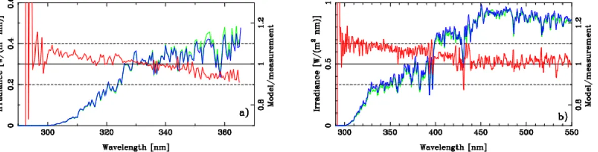
parison between measured and modelled irradiances. Hence, absolute agreement between the measurements and simulations must be ensured. In Fig. 1 is shown examples of measured and simulated spectra during cloudless conditions. The agree-ment between the measureagree-ments and the model simulations is within the uncertainties associated with the measurements and the simulations and is of the same magnitude

20

as that reported earlier byMayer et al.(1997);Kylling et al.(1998) andVan Weele et al.

(2000) for similar conditions. The ±5% differences between the measurements and the simulations gives uncertainties of around 10% in the derived cloud optical depth. The uncertainty is largest for optically thin clouds.

The cloud optical depths derived from the ground measurements were compared

25

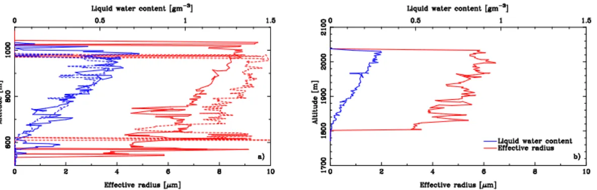
with in situ aircraft data for two days, days 257 and 263, when the sky was overcast. On both days the aircraft made several triangular patterns at constant altitudes above the ground stations and some profiles. Here attention is paid to the profile measurements. The liquid water content and the effective radius measured during the descent and

(12)

ACPD

5, 1421–1467, 2005

Full Screen / Esc

EGU

ascent around 12:00 UTC on day 257 and the ascent on day 263 are shown in Fig.2. Using the water cloud parameterization ofHu and Stamnes(1993) the profiles on day 257 yield total cloud optical depths of about 30.3 for the descent and 19.7 for the ascent for a wavelength of 380 nm. The cloud on day 263 was thinner with an optical depth of about 9.2. The differences in the optical depths on day 257 are mainly caused by

5

differences in r_e between the ascent (dashed line) and the descent (solid line). For shortwave radiation the water cloud volume extinction coefficient β_extis directly related to the liquid water content, LW C, and the droplet equivalent radius, r_e, (Stephens,

1978) β_ext≈ 3 2 LW C r_e . (1) 10

Thus, for a constant LW C, a reduction in r_eby a factor of 2 will double the cloud optical depth. The in situ measured r_e on day 263 is shown in Fig.2and varies between 4– 9 µm on day 257 and 3–6 µm on day 263. It is generally increasing with altitude. The sensitivity of the water cloud optical depth to r_e may be examplified by noting that for the ascent on day 257 the in situ optical depth was 19.7 at 380 nm. Using the same

15

LW C, but constant r_eof 5, 7.5 and 10 µm gives optical depths of 34.6, 22.7 and 16.9, respectively.

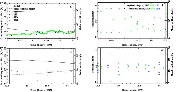
The effective cloud optical depths measured from the surface are shown in the right panel of Fig.3. For day 257 the cloud optical depths deduced from the NTN and GRT instruments were both around 38 at 12:00. At 11:40 the NTN optical depth was 32. On

20

day 263 the optical depths varied between 7 and 15 at the time the cloud profile was made (around 13:00). These optical depths are larger than the optical depths derived from the in situ aircraft measurements. One possible reason for the discrepancy is cloud horizontal inhomogeneties.

For day 257 the profile was made about 0.1◦ south of the NTN site and the wind

25

was blowing from the north. On day 263 the profile was made slightly east of the Weybourne site. Thus on both days cloud inhomogeneties may be part of the reason for the differences between the in situ and ground based cloud optical depths. Just

(13)

ACPD

5, 1421–1467, 2005

Full Screen / Esc

EGU

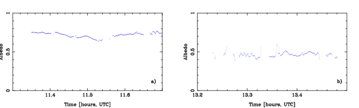
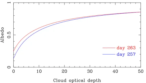
after the ascents on days 257 and 263, constant altitude legs were made above the clouds. The measured albedos derived from the Albedometer onboard the Partenavia, are shown in Fig.4. The albedo appears to exhibit relatively small variations. However, the cloud optical depth of the underlying cloud may still vary considerably. In Fig.5

is shown model simulations of the albedo as a function of cloud optical depth at the

5

two flight altitudes. The clouds vertical distribution were taken from Fig.2and the total optical depth scaled between 0 and 50. The solar zenith angles for the simulations were representative for the flight conditions. For day 257 the albedo varied between 0.65 and 0.75. This corresponds to cloud optical depths between about 15 and 25. Similar numbers for day 263 are 0.4–0.5 for the albedo and 2–6 for the cloud optical depth.

10

Thus, horizontal variations of the cloud may explain the differences between the in situ aircraft and the ground based cloud optical depths. Nevertheless, the optical depths estimated from the ground measurements gives a good indication of the horizontal variability over the domain and is used in the subsequent analysis.

5. Measurements versus simulations

15

Surface measurements were made continously in the period 12–29 September 2002. A number of flights were made during the same period. Here attention is paid to five days with clearly defined cloudless (1 day), completely overcast (2 days) and broken clouds periods (2 days), see Table3.

5.1. Cloudless situation

20

At the very first day of the main campaign, 12.9, day 255, the sky was partly overcast until about 12:00 UTC. It then cleared up and the sky became cloudless. Also, the VELIS lidar indicated that no subvisible cirrus was present. During the cloudless con-ditions flights were made over the ground stations in a triangular pattern. In addition the ground stations intensified their measurement schemes.

(14)

ACPD

5, 1421–1467, 2005

Full Screen / Esc

EGU

5.1.1. Ground data comparison

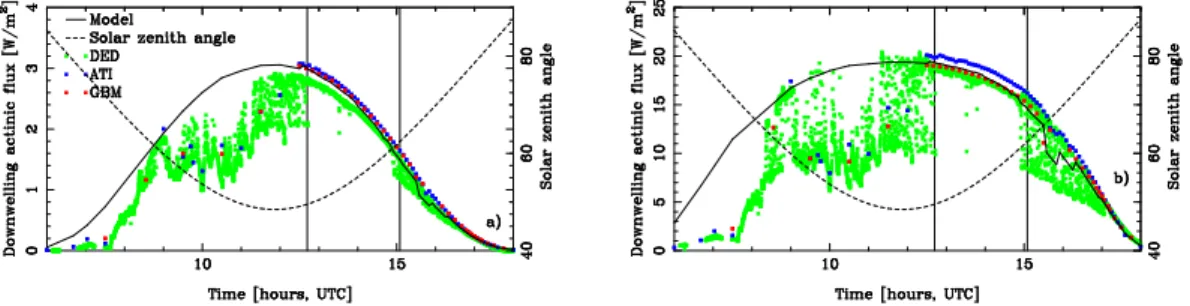
The time evolution of the downwelling actinic flux is shown in Fig.6. The downwelling actinic flux is shown for a wavelength region where ozone absorbs, 305–320 nm, left figure, and a wavelength region where ozone does not absorb, 380–400 nm, right fig-ure. The different diurnal behaviour of the actinic flux in these two wavelength regions

5

is evident. It is caused by the larger direct contribution to the total actinic flux at larger wavelengths. In addition to the measurements, simulations of the cloudless actinic flux are shown as well. The bump in the modelled clear sky actinic flux between 15:00 and 16:30 UTC is caused by significant increases, from about 0.05 to about 0.2, in the aerosol optical depth. For the integrated 380–400 nm wavelength range the DED

10

measurements are about 2–4% smaller, while the ATI measurements are 4–6% higher than the simulations. The GBM measurements are 0-2% lower than the simulations for the same range. For the integrated 305–320 nm range ATI and GBM are 3–5% higher then the model simulation, and DED is 3–5% lower. These spectral differences are also visible in individual spectra as shown in Fig.7 for the ATI and DED instruments

15

together with uvspec model simulations. The spectral resolution is higher for the spec-trum from the ATI insspec-trument. This is due to the spectral width of the slit function which is 0.5 and 2.2 nm at FWHM for the ATI and DED instruments respectively.

The measurement-model differences are of the same magnitude to those reported

by Fr ¨uh et al. (2003) for 2π ground-based measurements of the actinic flux and to

20

those reported byHofzumahaus et al.(2002). In the latter the 4π spectral actinic flux measured between 120 m to 13 000 m by an aircraft mounted spectroradiometer was compared to the same radiative transfer model used here. Considering the uncertain-ties in both the measurements and the simulations it is concluded that the simulations and the measurements agree within the uncertainties. Furthermore, the overall

agree-25

ment between the measurements and the model simulations of the actinic flux is similar to that for the irradiances presented in Fig.1.

(15)

ACPD

5, 1421–1467, 2005

Full Screen / Esc

EGU

irradiances shown in Fig.1. This is in agreement with the theoretical predicitions for these solar zenith angles and atmospheric conditions of e.g. Kylling et al. (2003b), their Figs. 1 and 2 and Eq. (7). It is noted that no simple relationship exists between the irradiance and the actinic flux.

5.1.2. Aircraft data comparison

5

The flights made during the cloudless period went up to an altitude of about 2000 m. The ascent starting at 13:60:68 and ending at 13:87:67 UTC was selected for further analysis. The solar zenith angle varied between 53.3◦ and 54.8◦ during the ascent. This variation in solar zenith angle caused less than 2% (6%) variations in the surface downwelling actinic flux in the UVA (UVB). This time slot is in the middle of the cloudless

10

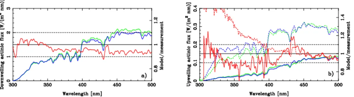
period, hence the data are minimally effected by possible clouds on the horizon. In Fig. 8is shown examples of the measured down- and upwelling actinic fluxes at some altitudes. Also shown are model simulations and model/measurement ratios. The downwelling measured and simulated actinic fluxes agree similar to the measured and simulated irradiances shown in Fig.1. The model overestimates by about 3–4%

15

below 320 nm and underestimates by 5–7% above about 350 nm. This is within the combined model and measurement uncertainties. The latter is estimated to ±8% in the UV range (305–400 nm) and ±4.9% in the visible (400–700 nm)(J ¨akel et al.,2005). For the upwelling spectra the disagreement between the model and measurements is larger. For the 58 m altitude spectrum the overall agreement is reasonable. Part of

20

the structure seen may be caused by unaccounted wavelength shifts. All ground and aircraft spectra, except the upwelling aircraft spectra, have been wavelength shift cor-rected with the SHICRIVM algorithm (Slaper et al.,1995). The model overestimates the upwelling spectrum at 1961 m significantly below about 380 nm. There is also a similar trend for the 58 m spectrum. Causes for the differences may be attributed to

25

several reasons. One is the non-perfect angular response of the input optics. This gives crosstalk between the upper and lower hemisphere. For low albedo and low alti-tude conditions the contributions from the upper hemisphere to the lower hemisphere

(16)

ACPD

5, 1421–1467, 2005

Full Screen / Esc

EGU

signal may be considerable, see Fig. 6 of Hofzumahaus et al. (2002). The angular response correction depend on altitude, wavelength, surface albedo and solar zenith angle. In addition, clouds and aerosol will affect the correction. The measurements have been corrected for the non-perfect angular response following the procedure of

J ¨akel et al.(2005). However, an ideal correction implies complete knowledge about the

5

sky radiance and that is not achievable. Also, the upwelling fluxes are rather sensitive to the albedo of the underlying surface. Uncertainties in the albedo estimate causes large changes in the upwelling radiation, especially for low altitudes and longer wave-lengths. However, since the agreement was reasonable at 58 m and the albedo is small for the conditions here, the albedo is not a likely cause for the differences at 1961 m.

10

Furthermore, uncertainties in the aerosol optical depth, single scattering albedo and asymmetry factor may affect the model results and most those for the upwelling actinic flux at 1961 m. Finally, during the ascent the acceleration of the aircraft was in periods outside the operational range of the stabilization system of the input optics. While the differences between the model and measurements are larger for the upwelling than the

15

downwelling actinic flux, it is noted that the magnitude of the upwelling actinic flux is much smaller than the downwelling actinic flux for a cloudless sky and a small albedo. Hence, the contribution to the 4π actinic flux is rather small from the upwelling part. Note that the FWHM of the DFD and DFU instruments is about 2.5 nm. Hence the spectra shown in Fig. 8 have similar spectral structure to those shown for the DED

20

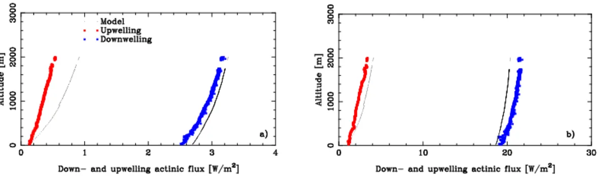
instrument in Fig.7. In Fig.9is shown vertical profiles of the measured and simulated up- and downwelling actinic fluxes integrated over the 380–400 nm and 305–320 nm wavelength intervals. The differences between the measured and simulated actinic fluxes reflects the spectral differences discussed above and shown in Fig.8. Both the down- and upwelling actinic fkuxes increase with altitude for both wavelength intervals

25

presented. The increase is largest for the upwelling actinic fluxes because as the alti-tude increase the amount of upscattered radiation increase due to Rayleigh scattering. The wavelength dependence of the Rayleigh scattering cross section also causes the increase in the upwelling actinic fluxes to be largest for short wavelengths. Similarily,

(17)

ACPD

5, 1421–1467, 2005

Full Screen / Esc

EGU

the decrease in the downwelling actinic flux is largest for the shortest wavelengths. Except for the upwelling actinic flux, the model and the measurement agree within their uncertainties for the cloudless case. Furthermore, the measurements made at the different ground stations agree within their uncertainties. With this in the mind, attention is turned to overcast situations.

5

5.2. Overcast

Two days, 14 and 20 September, were considered as “homogeneous” completely over-cast cases. Especially the 14 September was a “clean” situation with no cirrus above the stratocumulus cloud layer, see Table3.

10

In Fig.3is shown the time evolution of the measured actinic flux on the ground during the flights on these days. Also shown is the effective cloud optical depth as deduced from the surface irradiance measurements. Compared to the cloudless situation the actinic flux is reduced by about 75% (50%) on day 257 (263). The variability in the actinic flux during the flight hours indicates that the cloud was not horizontally

homo-15

geneous and the downwelling actinic flux at times exhibited differences of about 40% between the stations. These variations are also seen in the cloud optical depth and transmittance, right panel, Fig. 3. During the flight the wind was from the north and relatively strong.

20

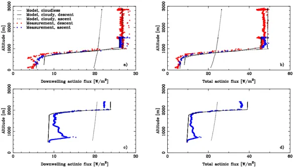
In Fig.10is shown the measured and simulated actinic fluxes as a function of altitude for the ascents (blue) and descent (red) on days 257 and 263. The lines are model simulations of the measurements. The effect of the clouds on the actinic flux is similar on both days. Above the cloud the actinic flux is enhanced, a maximum is observed just below the cloud top, and below the cloud the actinic flux is reduced compared

(18)

ACPD

5, 1421–1467, 2005

Full Screen / Esc

EGU

to the cloudless situation. The variability seen at about 2900 m for the descent (red points) and 1500 m for the ascent (blue points) are due to the aircraft spending some time at these altitudes, thus viewing different parts of the clouds. These variations thus indicate cloud horizontal inhomogeneities and their effect of about 11% on the downwelling and total actinic fluxes for these measurements.

5

The above cloud enhancement depends on the optical thickness of the cloud (see Fig. 9 ofVan Weele and Duynkerke,1993). The optical depth for the descent on day 257 was 30.3 and reduced to 19.7 for the ascent. A thicker cloud has a higher albedo, thus the above cloud actinic flux is higher for the descent, red points and dashed line in Fig. 10, compared to the ascent, blue points and solid line. Correspondingly, the

10

optically thicker cloud transmits less radiation resulting in lower below cloud radiation than the optically thinner cloud.

Just below the cloud top theory predicts a pronounced maximum in the actinic flux. This maximum is seen in both the measurements and the model simulations of the downwelling actinic flux on both days. Though, for the ascent on day 257 it is not seen.

15

This is thought to be due to lack of data in the topmost part of the cloud. As the model simulates individual data points, these enhanced points are missed in the simulation as well. Similar enhancements have been observed in tethered-balloon measurements byde Roode et al. (2001) and Vil `a–Gureau de Arellano et al. (1994). The maximum has theoretically been described byMadronich(1987) andVan Weele and Duynkerke

20

(1993). The effect disappears for large solar zenith angles. Furthermore, the magni-tude of the maximum increases with increasing cloud optical depth, while the geometric extent decreases with increasing cloud optical depth. The maximum occurs at optical depths were the direct beam is still significant and the diffuse radiation is becoming appreciable. Below the maximum the actinic flux decreases monotonically with

de-25

creasing altitude until cloud bottom. Below the cloud the actinic flux varies little with altitude. This is typically for the effect of clouds over surfaces with a low albedo. Over high albedo surfaces such as snow the behaviour is significantly different (de Roode

(19)

ACPD

5, 1421–1467, 2005

Full Screen / Esc

EGU

The overall agreement in Fig.10between the model simulations and the measure-ments is good. The simulations incorporates the main features of the measuremeasure-ments. However some differences are evident and especially below the cloud bottom where the model is consistently larger than the measurements. As shown in Fig.4the clouds were not homogeneous which clearly affected the radiation measurements. The

rela-5

tive differences in the transmittance between the stations were larger on day 263 com-pared to day 257, see Fig.3. This further indicates cloud horizontal inhomogeneities which may explain the larger below cloud differences for day 263 compared to day 257. The model simulations are 1-D and hence do not account for any horizontal variability. Compared to a cloudless atmosphere the cloud on day 257 increases the

down-10

welling actinic flux by about 30% above the cloud and reduces it by about 65% below. Similar numbers for the total actinic flux are about 100% and 55% respectively. The cloud on day 263 is thinner, hence more radiation penetrates the cloud and less is scattered back. The total (downwelling) flux is increased by about 60% (20%) above the cloud and reduced by about 55% (55%) below the cloud. These number for the

15

total actinic flux are in agreement with those reported by e.g.Vil `a–Gureau de Arellano

et al. (1994) andShetter and M ¨uller(1999). 5.3. Broken clouds

The above discussed cases may be considered “simple” 1-D. More complex cases include broken clouds, multi-layer clouds and combinations of these. On day 256 “cloud

20

bands” oriented west-east covered 4/8 over land. A snapshot of the cloud bands is provided in Fig.11. There was no cirrus on that day. Day 261 was a rather complex situation with quite inhomogeneous cumulus/stratus between 500 and 1900 m and 4/8 to 8/8 cirrus between 11 and 14 km. The cloud inhomogeneity was clearly visible from below, Fig.11. Two flights were made on day 256. Data from the second and longest

25

(20)

ACPD

5, 1421–1467, 2005

Full Screen / Esc

EGU

In Fig. 12 is shown the downwelling actinic flux measured on the ground on these two days during the flights. Also shown are the effective cloud optical depths and transmittances as deduced from the ground measurements. On day 256 the cloud bands were only present inland. This is seen in Fig. 12 as the measurements by

5

the ATI and GBM instruments on the coast are representative of cloudless conditions. The inland measurements by the DED instrument varies rapidly as the cloud bands pass over the measurement site. Occassionally the measurements are larger then the cloudless model simulations shown as a solid black line. This indicates the combined effect of scattering off cloud sides and a visible solar disk (Mims and Frederick,1994;

10

Nack and Green,1974). The variations seen in the actinic flux of the DED instrument is also evident in the transmittance and cloud optical depths deduced from the inland GRT and NTN instruments. Note however, that the time resolution of these instruments are lower than for the DED instrument. Both episodes of cloud gaps and cloud bands are readily identified in Fig.12. The steps in the cloudless model results, black solid

15

lines, are due to changes in the aerosol optical depth deduced from VELIS.

On the ground less variations are seen at the individual stations on day 261, Fig.12. However, the variations between the stations is of the same magnitude as the variations at Aylsham, DED, on day 256. Thus, while the sky appeared to be more homogeneous on day 261 compared to day 256, Fig.11, the cloud inhomogeneties caused

consider-20

able variations over the area covered by the ground stations. This is also evident in the albedo measurements shown in Fig.13. Most of time the aircraft is above the clouds. The parts within the clouds is readily identified by large and spurious variations in the albedo. These are during the ascents and descents at the beginning and end of both flights and around 1400 for the flight on day 256. For both days the large variations in

25

the albedo measured while the aircraft was above the clouds, reflect the horizontal in-homogeneties of the clouds. For day 256 the minimum albedo is close to the cloudless albedo while the maximum albedo reflects that the clouds were not optically thick on

(21)

ACPD

5, 1421–1467, 2005

Full Screen / Esc

EGU

this day. On the other hand, the clouds on day 261 were thicker with smaller and fewer gaps. Thus the higher minimum and maximum albedos.

In order to simulate the measurements vertical profiles of the liquid water content and effective droplet radius are required. As the clouds were inhomogeneous it was not

5

possible to select data from a single cloud penetration as done above for days 257 and 263. Instead all liquid water content data from the PVM and all effective radius data from the Fast-FSSP were plotted as a function of altitude, Fig.14. For the cloud band, day 256, it was assumed that the cloud was vertically homogeneous with a liquid water content of 0.5 gm3and r_e=5.5 µm. Cloud bottom was at 900 m and cloud top at 930 m.

10

With theHu and Stamnes(1993) parameterization this resulted in a cloud optical depth of 4.3 at 380 nm. The optical depths derived from the ground measurements varied between 10 and 16 when clouds were overhead, Fig. 12. As discussed earlier this difference may be caused by cloud horizontal inhomogeneties.

For day 261 the clouds had a larger vertical extension. A near adiabatic liquid water

15

profile was assumed and values between the maximum and minimum measured liquid water contents adopted. The r_ewas asssumed to increase with altitude, Fig.14. This resulted in an optical depth of 31.7 at 380 nm. The inland ground deduced optical depths varied between 20 and 25 which, again considering horizontal variations, is consistent with the cloud built from the PVM and Fast-FSSP measurements.

20

In Fig. 15 the total and downwelling actinic fluxes measured by the Partenavia on days 256 and 261 are shown as a function of altitude. Also shown are model simula-tions for cloudless and cloudy condisimula-tions. For the cloudy simulasimula-tions the cloud prop-erties shown in Fig.14 were used. As mentioned earlier day 256 was characterised by cloud bands oriented west-east. Thus, from the ground it was either overcast or

25

the sun could be seen. The flight on day 256 lasted for about 2.5 h. During this time period the solar zenith angle increased from about 52◦to 65◦. This changed the actinic fluxes by about 30% below the cloud and about 25% for the cloudless conditions. The

(22)

ACPD

5, 1421–1467, 2005

Full Screen / Esc

EGU

variability seen in the actinic fluxes of about ±10% when the aircraft was at constant altitude above the clouds, reflects the changes in the cloud cover underneath. See for example the horizontally oriented data points at about 1600, 2300 and 2800 m in the upper panels of Fig. 15. The ground measurements on day 256 of the downwelling actinic flux varies between 6 and 19 W/m2, Fig.12. This is in agreement with the below

5

cloud aircraft measurements, Fig.15. Above the cloud the aircraft measurements are 0–150% larger than the cloudless ground measurements.

For day 261 the picture is more complicated due to the horizontal and vertical varia-tions of the cloud cover. The cloud simulavaria-tions obviously has the cloud bottom placed a little too high. The ground measurements varied between 3 and 16 W/m2, Fig. 12.

10

The same variability is not seen in the aircraft data. However, this is caused by the fact that only one ascent and descent was made on that day. Thus, the aircraft data may not be fully representative for the whole area in its full vertical extent.

As can be seen in Fig.15 the measurements lie between the cloudless, F_clear, and cloudy, F_cloudy, 1-D model simulations. Thus, for this situation a simple cloud fraction,

15

C_f, approximation

F = C_fF_cloudy+ (1 − C_f)F_clear (2)

might yield representative values for the total actinic flux, F , provided that the vertical extent of the cloud and its optical properties were known, and that a realistic value of C_f is available. For day 256 values of 0.3 (green), 0.5 (red) and 0.7 (purple) were

20

used for C_f. The above cloud actinic flux is reasonably well captured by any of these cloud fractions. However, below the cloud the actinic flux is either represented by cloudless or overcast calculations. Thus the cloud fraction approximation appears to only capture part of the picture for this situation. For day 261 values of 0.5 (green), 0.6 (red) and 0.7 (purple) were used for C_f. The overall best agreement both above and

25

below the cloud is obtained with a value of 0.6 although the below cloud actinic flux is slightly overestimated. The best agreement below the cloud is obtained for C_f=0.8 (not shown). However a value of 0.8 overestimates the actinic flux above the cloud. Thus, the cloud fraction approach appears to be too simple to describe both the above cloud

(23)

ACPD

5, 1421–1467, 2005

Full Screen / Esc

EGU

enhancement and the below cloud reduction by a single number. It must also be noted that during such inhomogeneous and changing conditions it is not feasible to sample a larger area with aircrafts. Thus the measured data may not be fully representative for the area under investigation.

Based on the images shown in Fig.11 the cloud amounts are estimated to 4 oktas

5

on day 256 and values between 7–8 oktas for day 261. The relationship between cloud amount as estimated by a surface observer and the earthview (vertical) cloud amount needed in radiative transfer models has been discussed by Henderson-Sellers and

McGuffie (1990) and references therein. For mid-range cloud amounts the two views are comparable. This agrees with the findings here that a C_f=0.5 gives a reasonable

10

representation above the cloud for day 256. For large cloud amount surface observa-tions tends to overestimate cloud amount as compared to the earthview cloud amount. This is also found here as a value of C_f=0.9, or about 7 oktas, overestimates the ac-tinic flux by about 16% above the cloud and underestimates the acac-tinic flux by about 33% below the cloud compared to C_f=0.6. Thus, while allsky images are useful to

15

document the measurement conditions and in the selection of interesting cases, direct use of cloud amounts deduced from these images must be used with care in models.

6. Conclusions

As part of the INSPECTRO project an extensive campaign to study the influence of clouds on the spectral actinic flux in the lower troposphere was carried out in East

20

Anglia, UK, September 2002. The spectral actinic flux, the irradiance and aerosol and cloud properties were measured by aircraft and four ground stations.

Data from cloudless, broken cloud and overcast situations were selected for analy-sis. A detailed radiative transfer model was used to simulate and interpret the mea-surements. The following findings were made.

25

(24)

ACPD

5, 1421–1467, 2005

Full Screen / Esc

EGU

flux were reproduced by the radiative transfer model within the measurement and model uncertainties of about ±5%.

– For cloud conditions visually characterised as horizontally homogeneous the

downwelling actinic flux at the surface at times varied by up to 40% between stations for the rather small experimental area of about 12×12 km2.

Simultane-5

ously the above cloud variations in the downwelling and total actinic fluxes were about 11% over the area.

– For overcast situations 1-D radiative transfer calculations reproduced the overall

behaviour of the actinic flux measured by the aircraft. Especially the above cloud enhancement and below cloud reductions are well characterized.

10

– The above cloud enhancement increases with increasing optical depth. Similarily,

the below cloud reduction increases with increasing optical depth.

– Just below the cloud top the downwelling actinic flux has a maximum which is

seen in both the measurements and the model results.

– For broken cloud situations the cloud fraction approach captures some of the

15

changes in the actinic flux. However, no single value for the cloud fraction is able to reproduce the measured above cloud enhancement and below cloud reduc-tions for the analysed situareduc-tions.

Thus, we conclude that for the cases studied here, cloudless and overcast single-layered clouds may be satisfactorily simulated by 1-D radiative transfer models. The

20

relatively simple broken cloud cases investigated indicates that for these cloud situa-tions and more complex cases 3-D correcsitua-tions must be applied. What these correc-tions look like is an outstanding research question.

As part of the INSPECTRO project a second campaign was conducted in May 2004 in southern Germany covering a larger, about 50×50 km2, area to further elucidate the

25

(25)

ACPD

5, 1421–1467, 2005

Full Screen / Esc

EGU

Acknowledgements. This research was funded by contract EVK2-CT-2001-00130 from the

Eu-ropean Commission. Funding by the German Science Foundation (DFG) and the German Research Ministry (BMBF) are acknowledged. Part of this research was performed while one of the authors (M.W.) held a National Research Council Research Associateship Award at the NASA Ames Research Center. As usual the enviscope GmbH company and the pilot of the

5

Partenavia, Bernd Schumacher, did an excellent job in preparing and conducting the measure-ments with the Partenavia.

References

Anderson, G., Clough, S., Kneizys, F., Chetwynd, J., and Shettle, E.: AFGL atmospheric constituent profiles (0–120 km), Tech. Rep. AFGL-TR-86-0110, Air Force Geophys. Lab.,

10

Hanscom Air Force Base, Bedford, Mass., 1986. 1428

Anderson, G. P., Chetwynd, J. H., Theriault, J.-M., Acharya, P. K., Berk, A., Robertson, D. C., Kneizys, F. X., Hoke, M. L., Abreu, L. W., and Shettle, E. P.: MODTRAN2: Suitability for remote sensing, in Atmospheric Propagation and Remote Sensing, SPIE Conf. Ser.: vol. 1968, edited by: Kohnle, A. and Miller, W. B. 514–525, Soc. of Photo–Optical–Instrum. Eng.,

15

Bellingham, Wash., 1993. 1429

Bais, A. F., Madronich, S., R., J. C. S., Hall, J., Mayer, B.: van Weele, M., G., J. L. J., Calvert, Cantrell, C. A., Shetter, R. E., Hofzumahaus, A., Koepke, P., Monks, P. S., Frost, G., McKenzie, R., Krotkov, N., Kylling, A., Swartz, W. H., Lloyd, S., Pfister, G., Martin, T. J., Roeth, E.-P., Griffioen, E., Ruggaber, A., Krol, M., Kraus, A., Edwards, G. D., Mueller,

20

M., Lefer, B. L., Johnston, P., Schwander, H., Flittner, D., Gardiner, B. G., Barrick, J., and Schmitt, R.: International Photolysis Frequency Measurement and Model Intercomparison (IPMMI): Spectral actinic solar flux measurements and modeling, J. Geophys. Res., 108, doi:10.1029/2002JD002891, 2003. 1429

Barnaba, F. and Gobbi, G.: Modeling the aerosol extinction versus backscatter relationship in

25

a mixed maritime-continental atmosphere: Lidar application and validation, J. Atm. Ocean Technol., 21, 428–442, 2004. 1427

Bass, A. M. and Paur, R. J.: The ultraviolet cross-section of ozone, I, The measurements, in: Atmospheric Ozone: Proceedings of the Quadrennial Ozone Symposium, edited by: Zerefos, C. S. and Ghazi, A., 601–606, D. Reidel, Norwell, Mass., 1985. 1428

(26)

ACPD

5, 1421–1467, 2005

Full Screen / Esc

EGU

Brasseur, A.-L., Ramaroson, R., Delannoy, A., Skamarock, W., and Barth, M.: Three-dimensional calculation of photolysis frequencies in the presence of clouds and impact on photochemistry, J. of Atmospheric Chemistry, 41, 211–237, 2002. 1425

Cahalan, R. F., Ridgway, W., Wiscombe, W. J., Gollmer, S., and Harshvardhan: Independent pixel and Monte Carlo estimates of stratocumulus albedo, J. Atmos. Sci., 51, 3776–3790,

5

1994. 1424

Chambers, L. H., Wielicki, B. A., and Evans, K. F.: Accuracy of the independent pixel approx-imation for satellite estimates of oceanic boundary layer cloud optical depth, J. Geophys. Res., 102, 1779–1794, 1997. 1425

Crawford, J., Shetter, R., Lefer, B., Cantrell, C., Junkermann, W., Madronich, S., and Calvert,

10

J.: Cloud impacts on UV spectral actinic flux observed during the International photoly-sis frequency measurement and model intercomparison (IPMMI), J. Geophys. Res., 108, doi:10.1029/2002JD002731, 2003. 1425

Dahlback, A. and Stamnes, K.: A new spherical model for computing the radiation field available for photolysis and heating at twilight, Planet. Space Sci., 39, 671–683, 1991. 1429

15

de Roode, S. R., Duynkerke, P. G., Boot, W., and der Hage, J. C. H. V.: Surface and tethered-balloon observations of actinic flux: effects of arctic stratus, surface albedo, and solar zenith angle, J. Geophys. Res., 106, 27 497–27 507, 2001. 1437

Evans, K. F.: The spherical harmonics discrete ordinate method for three–dimensional atmo-spheric radiative transfer, J. Atmos. Sci., 55, 429–446, 1998. 1425

20

Fr ¨uh, B., Trautmann, T., Wendisch, M., and Keil, A.: Comparison of observed and simulated NO₂ photodissociation frequencies in a cloudless atmosphere and continental boundary layer clouds, J. Geophys. Res., 105, 9843–9857, 2000. 1424

Fr ¨uh, B., Eckstein, E., Trautmann, T., Wendisch, M., Fiebig, M., and Feister, U.: Ground-based measured and calculated spectra of actinic flux density and downward UV irradiance in

25

cloudless conditions and their sensitivity to aeosol microphysical properties, J. Geophys. Res., 108, doi:10.1029/2002JD002933, 2003. 1433

Gobbi, G. P., Barnaba, F., Giorgi, R., and Santacasa, A.: Altitude-resolved properties of a Sa-haran dust event over the Mediterranean, Atmospheric Environment, 34, 5119–5127, 2000.

1427

30

Gobbi, G. P., Barnaba, F., and Ammannato, L.: The vertical distribution of aerosols, Saharan dust and cirrus clouds at Rome (Italy) in the year 2001, Atmos. Chem. Phys., 4, 351–359, 2004,

(27)

ACPD

5, 1421–1467, 2005

Full Screen / Esc

EGU

SRef-ID: 1680-7324/acp/2004-4-351. 1427

Henderson-Sellers, A. and McGuffie, K.: Are cloud amounts estimated from satellite sensors and conventional surface-based observations related?, Int. J. Remote Sensing, 11, 543–550, 1990. 1442

Hofzumahaus, A., Kraus, A., Kylling, A., and Zerefos, C.: Solar actinic radiation (280-420 nm)

5

in the cloud-free troposphere between ground and 12 km altitude: Measurements and model results, J. Geophys. Res., 107, doi:10.1029/2001JD900142, 2002. 1429,1433,1435

Hu, Y. X. and Stamnes, K.: An accurate parameterization of the radiative properties of water clouds suitable for use in climate models, J. of Climate, 6, 728–742, 1993. 1431,1440

J ¨akel, E., Wendisch, M., Kniffka, A., and Trautmann, T.: A new airborne system for fast

mea-10

surements of up- and downwelling spectral actinic flux densities, Appl. Opt., 44, 434–444, 2005. 1427,1434,1435

Junkermann, W.: Measurements of the J(O1D) actinic flux within and above stratiform clouds and above snow surfaces, Geophys. Res. Lett., 21, 793–796, 1994. 1424

Kelley, P., Dickerson, R. R., Luke, W. T., and Kok, G. L.: Rate of NO₂photolysis from the surface

15

to 7,6 km altitude in clear-sky and clouds, Geophys. Res. Lett., 22, 2621–2624, 1995. 1424

Kylling, A., Bais, A. F., Blumthaler, M., Schreder, J., Zerefos, C. S., and Kosmidis, E.: The effect of aerosols on solar UV irradiances during the Photochemical Activity and Solar Ultraviolet Radiation campaign, J. Geophys. Res., 103, 26 051–26 060, 1998. 1429,1430

Kylling, A., Danielsen, T., Blumthaler, M., Schreder, J., and Johnsen, B.: Twilight tropospheric

20

and stratospheric photodissociation rates derived from balloon borne radiation measure-ments, Atmos. Chem. Phys., 3, 377–385, 2003a,

SRef-ID: 1680-7324/acp/2003-3-377. 1428

Kylling, A., Webb, A. R., Bais, A. F., Blumthaler, M., Scmitt, R., Thiel, S., Kazantzidis, A., Kift, R., Misslbeck, M., Schallhart, B., Schreder, J., C.Topaloglou, Kazadzis, S., and

Rim-25

mer, J.: Actinic flux determination from measurements of irradiance, J. Geophys. Res., 108, doi:10.1029/2002JD003236, 2003b. 1434

Los, A., van Weele, M., and Duynkerke, P. G.: Actinic fluxes in broken cloud fields, J. Geophys. Res., 102, 4257–4266, 1997. 1425

Madronich, S.: Photodissociation in the atmosphere 1. Actinic flux and the effects of ground

30

reflections and clouds, J. Geophys. Res., 92, 9740–9752, 1987. 1423,1424,1437

Mayer, B., Seckmeyer, G., and Kylling, A.: Systematic long–term comparison of spectral UV measurements and UVSPEC modeling results, J. Geophys. Res., 102, 8755–8767, 1997.

(28)

ACPD

5, 1421–1467, 2005

Full Screen / Esc

EGU

1429,1430

Mims, F. M. I. and Frederick, J. E.: Cumulus clouds and UV-B, Nature, 371, 291, 1994. 1423,

1439

Monks, P. S., Rickard, A. R., Hall, S. L., and Richards, N. A. D.: Attenuation of spectral actinic flux and photolysis frequencies at the surface through homogenous cloud fields, J. Geophys.

5

Res., 109, doi:10.1029/2003JD004076, 2004. 1425

Nack, M. L. and Green, A. E. S.: Influence of clouds, haze, and smog on the middle ultraviolet reaching the ground, Appl. Opt., 13, 2405–2415, 1974. 1439

Nicolet, M.: On the molecular scattering in the terrestrial atmosphere: An empirical formula for its calculation in the homosphere, Planet. Space Sci., 32, 1467–1468, 1984. 1428

10

Ramanathan, V., Cess, R. D., Harrison, E. F., Minnis, P., Barkstrom, B. R., Ahmad, E., and Hartmann, D.: Cloud–radiative forcing and climate: results from the Earth radiation budget experiment, Science, 243, 57–63, 1989. 1423

Schwander, H., Koepke, P., and Ruggaber, A.: Uncertainties in modeled UV irradiances due to limited accuracy and availability of input data, J. Geophys. Res., 102, 9419–9429, 1997.

15

1429

Shetter, R. E. and M ¨uller, M.: Photolysis frequency measurements using actinic flux spectrora-diometry during the PEM–Tropics mission: instrumentation description and some results, J. Geophys. Res., 104, 5647–5661, 1999. 1424,1438

Slaper, H., Reinen, H. A. J. M., Blumthaler, M., Huber, M., and Kuik, F., Comparing ground–

20

level spectrally resolved solar UV measurements using various instruments: A technique resolving effects of wavelengths shift and slit width, Geophys. Res. Lett., 22, 2721–2724, 1995. 1434

Stamnes, K., Tsay, S.-C., Wiscombe, W., and Jayaweera, K.: Numerically stable algorithm for discrete–ordinate–method radiative transfer in multiple scattering and emitting layered

25

media, Appl. Opt., 27, 2502–2509, 1988. 1429

Stamnes, K., Slusser, J., and Bowen, M.: Derivation of total ozone abundance and cloud effects from spectral irradiance measurements, Appl. Opt., 30, 4418–4426, 1991. 1429

Stephens, G. L.: Radiation profiles in extended water clouds. II: Parameterization schemes, J. Atmos. Sci., 35, 2123–2132, 1978. 1431

30

Stephens, G. L. and Tsay, S.-C.: On the cloud absorption anomaly, Q. J. R. Meteorol. Soc., 116, 671–704, 1990. 1425

(29)

unpol-ACPD

5, 1421–1467, 2005

Full Screen / Esc

EGU

luted troposphere, J. Geophys. Res., 89, 1341–1349, 1994. 1423

Trautmann, T., Podgorny, I., Landgraf, J., and Crutzen, P. J.: Actinic fluxes and photodissoci-ation coefficients in cloud fields embedded in realistic atmospheres, J. Geophys. Res., 104, 30 173–30 192, 1999. 1425

Van Weele, M. and Duynkerke, P. G.: Effect of Clouds on the Photodissociation of NO₂:

obser-5

vations and modelling, J. of Atmospheric Chemistry, 16, 231–255, 1993. 1437

Van Weele, M., Martin, T. J., Blumthaler, M., Brogniez, C., den Onter, P. N., Engelsen, O., Lenoble, J., Mayer, B., Pfister, G., Ruggaber, A., Walravens, B., Weihs, P., Gardiner, P. G., Gillotay, D., Haferl, D., Kylling, A., Seckmeyer, G., and Wauben, W. M. F.: From model intercomparison towards benchmark UV spectra for six real atmospheric cases, J. Geophys.

10

Res., 105, 4916–4925, 2000. 1429,1430

V ´arnai, T. and Davies, R.: Effects of cloud heterogeneities on shortwave radiation: comparison of cloud-top variability and internal heterogeneity, J. Atmos. Sci., 56, 4206–4224, 1999. 1425

Vil `a–Gureau de Arellano, J., Duynkerke, P. G., and van Weele, M., Tethered–balloon mea-surements of actinic flux in a cloud–capped marine boundary layer, J. Geophys. Res., 99,

15

3699–3705, 1994. 1424,1437,1438

Webb, A. R., Bais, A. F., Blumthaler, M., Gobbi, G.-P., Kylling, A., Schmitt, R., Thiel, S., Barn-aba, F., Danielsen, T., Junkermann, W., Kazantzidis, A., Kelly, P., Kift, R., Liberti, G. L., Misslbeck, M., Schallhart, B., Schreder, J., and Topaloglou, C.: Measuring spectral actinic flux and irradiance: Experimental results from the ADMIRA (Actinic Flux Determination from

20

Measurements of Irradiance), J. Atm. Ocean Technol., 19, 1049–1062, 2002. 1427

Webb, A. R., Kylling, A., Wendisch, M., and J ¨akel, E.: Airborne measurements of ground and cloud spectral albedos under low aerosol loads, J. Geophys. Res., 109D, D20205, doi:10.1029/2004JD004768, 2004. 1428,1429

Weihs, P. and Webb, A. R.: Accuracy of spectral UV model calculations, 1, Consideration of

25

uncertainties in input parameters, J. Geophys. Res., 102, 1541–1550, 1997. 1429

Wendisch, M. and Mayer, B.: Vertical distribution of spectral solar irradiance in the cloudless sky: A case study, Geophys. Res. Lett., 30(4), 1183, doi:10.1029/2002GL016529, 2003.

1427,1429

Wendisch, M., M ¨uller, D., Schell, D., and Heintzenberg, J.: An airborne spectral albedometer

30

with active horizontal stabilization, J. Atm. Ocean Technol., 18, 1856–1866, 2001. 1427

Wendisch, M., Pilewskie, P., J ¨akel, E., Schmidt, S., Pommier, J., Howard, S., Jonsson, H. H., Guan, H., Schr ¨oder, M., and Mayer, B.: Airborne measurements of areal

(30)

spec-ACPD

5, 1421–1467, 2005

Full Screen / Esc

EGU

tral surface albedo over different sea and land surfaces, J. Geophys. Res., 109, D08 203, doi:10.1029/2003JD004393, 2004. 1427

Woods, T. N., Prinz, D. K., Rottmann, G. J., London, J., Crane, P. C., Cebula, R. P., Hilsenrath, E., Brueckner, G. E., Andrews, M. D., White, O. R., VanHoosier, M. E., Floyd, L. E., Herring, L. C., Knapp, B. G., Pankrantz, C. K., and Reiser, P. A.: Validation of the UARS solar ultravi-olet irradiances: Comparison with the Atlas 1 and 2 measurements, J. Geophys. Res., 101,

740

(31)

ACPD

5, 1421–1467, 2005

Full Screen / Esc

EGU

Table 1. Location of the ground stations and the type of measurements made at the respective

stations. For explanation of the acronyms see Table2.

Place Latitude Longitude measurements

Weybourne 52 57 02 N 01 07 18 E actinic flux (ATI), irradiance (ATI), lidar, chemistry Beeston Regis 52 56 15 N 01 16 00 E actinic flux (GBM), irradiance (GBM)

Briston 52 50 30 N 01 05 00 E actinic flux (DEG), irradiance (DEG,GRT) Aylsham 52 46 20 N 01 13 50 E actinic flux (DED), irradiance (NTN)