Drawing driver's attention to potentially dangerous objects

Drawing Driver's Attention to Potentially

Dangerous Objects

by

Orcun Kurugol

Submitted to the Department of Mechanical Engineering

in partial fulfillment of the requirements for the degree of

Master of Science in Mechanical Engineering

at the

MASSACHUSETTS INSTITUTE OF TECHNOLOGY

May 29008

Vay

2008

@ Massachusetts Institute of Technology 2008. All rights reserved.

A uthor ...

Dri~artment of Mechanical Engineering

May 16, 2008

Certified by...

...

Ichiro Masaki

Principle Research Associate

Certified by...

Thesis Supervisor

Berthold K.P. Horn

Professor of Computer Science and Engineering

A ,

Thesis Supervisor

Certified by..

John J. Leonard

Professor of Mechanical Engineering

dv• ..

Thesis Supervisor

Accepted by ... ... ... ...

JUL 29 2008

LIBRARIES

Lallit Anand

n, Department Committee on Graduate Students

Drawing Driver's Attention to Potentially Dangerous

Objects

by

Orcun Kurug1l

Submitted to the Department of Mechanical Engineering on May 19, 2008, in partial fulfillment of the

requirements for the degree of

Master of Science in Mechanical Engineering

Abstract

Drivers often have difficulties noticing potentially dangerous objects due to weather or lighting conditions or when their field of view is restricted. This thesis presents a display method for potentially dangerous objects to assist drivers in noticing dan-gerous situations. The object segment is denoised by adaptive thresholding, and the contrast, brightness and color of the segment are enhanced in order to make the object more noticeable. The contrast of the background is reduced to increase the effect of enhancement, and dynamic effects like changing the enhancement window size, window location, contrast, and brightness are added to increase the detectibil-ity of the object by the driver. Experiments showed that our method increased the perceptibility of potentially dangerous objects.

Thesis Supervisor: Ichiro Masaki Title: Principle Research Associate Thesis Supervisor: Berthold K.P. Horn

Title: Professor of Computer Science and Engineering Thesis Supervisor: John J. Leonard

Acknowledgments

I would like to thank Prof. Berthold K.P. Horn, Dr. Ichiro Masaki, and Prof. John J. Leonard for giving me precious guidance and advice for this thesis. I also want to thank Honda Motor Company for suppying data, and TUBiTAK for their sup-port. Thanks to all my friends, and especially ilke Kalcio'lu for being so patient and supportive. Above all, I would like to thank my family for their encouragement and unconditional love.

Contents

1 Introduction 7

2 Wavelets 9

2.1 Denoising via W avelets ... 12

2.2 Image Enhancement ... 14

3 Using Wavelet Enhancement on Images 18 3.1 Im age Layout ... 20

3.2 Using Coarse Image Data as the Background . ... 21

3.3 W indow Size Changes ... 23

3.4 Contrast Changes ... 25

3.5 Other Dynamic Effects ... 27

4 Experimental Results 31 5 Conclusion 39 5.1 Conclusion ... ... .. ... .. .... ... . .. .. ... . 39

List of Figures

2-1 Tiling of time-frequency space: Tiling by STFT is shown in (a), and by wavelets is shown in (b). In both figures horizontal axis is time axis, and vertical axis is frequency axis . ... . . . . . 10 2-2 2-D Wavelet Transform. H: Scaling filter, G: Wavelet filter, 21:

Down-sam pling by 2 ... . ... 12 2-3 Enhancement Functions. Black curve: El(v), Magenta curve: E2 (v),

Cyan curve: E(v) ... 15

3-1 Darkening camera views: On (a) the car on the left camera view is detected. However on (b) the car on left view is obscured by the truck, so detection algorithm detects no objects on the left image, and it is darkened ... 21 3-2 Effect of background contrast change: Original image is shown in (a),

(b) has the enhanced image on original background, (c) has the en-hanced image on first level coarse background, (d) has the enen-hanced image on second level coarse background . ... 22 3-3 Problem with the perspective projection when the object is enlarged.

Vehicle Vo will receive its twice size in the image when it is in the place of vehicle Vr. When the enlarged segment of Vo is placed by centering the original segment, it will be perceived as if it is in the place of vehicle Vp... 29

3-4 A vehicle following the trajectory k1 will be perceived as if it is follow-ing the trajectory k2, when its enlarged segment is placed by centerfollow-ing

the original segment. ... 30

4-1 Scaling and wavelet functions of sym-6 . ... 31

4-2 Denoising result of a night scene ... 33

4-3 Enhancement result of a hazy scene . ... 34

4-4 Enhancement result of an MRI image. . ... . . . . 35

4-5 Original image sequence ... 35

4-6 Expanding window size ... 36

4-7 Shrinking window size ... 36

4-8 Increasing contrast ... 37

4-9 Decreasing contrast ... ... 37

4-10 Moving window . ... . . . ... 38

Chapter 1

Introduction

Image processing has become a common tool in the last few decades for assisting drivers in recognizing dangerous situations around them [6, 9, 11, 20]. Especially at the cross-roads, the field of view of the driver is limited. This makes the exhibition of dangerous objects on the side roads in images obtained from cameras a necessity for safer driving. The methods of display of these objects are as important as their detection; an object which is detected by an algorithm, but not noticed by the driver is no better than an undetected object. Therefore, designing a method which can draw the attention of the driver to detected objects is crucial.

A widely used technique to draw attention to a detected object is to put a bounding box around it. However, although detection algorithms perform well, they are not perfect, and there can be false positives. Hence, car companies need display systems which are powerful enough to draw the driver's attention to potentially dangerous objects in the image and yet do not disturb the driver significantly when errors occur in the detection process. Instead of using a bounding box, change in image features in certain regions of the image which create differences relative to the rest of the image also can draw the driver's attention to those regions. Examples of such change in features can be enhancement of contrast, brightness, or color.

A good way of enhancing images is to work on image features in multiple scales. Jobson [12] worked on multiscale retinex, Laine [13], Lina [14], Zong [23], Bronnikov [2], and Sakel [18] used wavelets for denoising and enhancement, and Starck [19]

worked on a wavelet-like transform called curvelet transform. Chang [3], and Temizel [22] also achieved resolution enhancement using wavelets. In this thesis, wavelets are used, since they provide a good representation of spatial and frequency domains. In addition, wavelet transformation is fast.

In the previous studies, wavelet enhancement was implemented in the whole im-age. In this thesis, if the scene is hazy, the whole image was enhanced; otherwise wavelet enhancement was only implemented in manually segmented areas of the im-age. Enhancement of image segment enables other methods to be used to increase the effect of enhancement. Therefore, effect of changing the background contrast and brightness, and dynamic effects such as varying the size or the position, and the contrast or the brightness of the segment over a time period were also studied.

Wavelet transform, and denoising and enhancement algorithms in the wavelet do-main are discussed in the next chapter. In chapter 3, wavelet denoising and enhance-ment on images are presented, and methods for increasing the effect of enhanceenhance-ment are described. After the methodology is introduced, some examples of experimental results are displayed. At the end, a concise conclusion is presented with a discussion of suggested future work.

Chapter 2

Wavelets

Wavelet transforms provide a way of 'tiling' time-frequency space, or in the 2-D case of images, pixel position-spatial frequency space. One general method for tiling this space is Windowed Fourier Transform, or Short Time Fourier Transform (STFT); however, the STFT has a drawback; the basis functions of the Fourier Transform are sine and cosine which are not localized in space. In order to achieve localization in space, sine and cosine functions must be truncated with a window of particular width. Therefore, the resolution of analysis of the STFT in frequency and space is the same everywhere [10]. In distinction, a wavelet transform has basis functions derived from a 'mother wavelet', and these basis functions are localized in space. Because of this localization property, the window shape of the wavelet transform varies, and this gives it the advantage of having better frequency resolution for low frequencies and better time resolution for high frequencies. This makes sense, since low frequency signals last long and high frequency signals are short. An example of tiling of the time-frequency space by the STFT and wavelet transform is given in Figure 2-1.

As explained above, wavelet transforms have an infinite set of basis functions based on scaled versions of a 'mother wavelet' and mother wavelets can be chosen based on their known properties. The basis functions of wavelet transform are called scaling function which serves as a low-pass filter, and wavelet function which reveals the details of the processed signal. Orthonormal wavelets are a good choice, since they can be used for multi-resolution analysis, and their ease of use in analysis and

VWP\YM

evN

<V

/n

Figure 2-1: Tiling of time-frequency space: Tiling by STFT is shown in (a), and by wavelets is shown in (b). In both figures horizontal axis is time axis, and vertical axis is frequency axis

reconstruction steps. Also compactly supported continuous orthonormal wavelets are desirable, because the computation with them need not be truncated, and the asso-ciated decomposition and reconstruction algorithms are computationally faster and more precise [1, 21]. These wavelet families are called orthogonal, because their scal-ing function and wavelet function form an orthonormal basis. Daubechies' wavelets are a family of orthonormal wavelets which are continuous and have compact support. Also symmetry is a desirable property to work on images; therefore, Daubechies' Least Asymmetric Wavelets (Symlets) were chosen as the wavelet family in this thesis.

Since images on a computer are discrete, a Discrete Wavelet Transform (DWT) should be used to in order to find the wavelet coefficients. Once the mother wavelet is chosen, the weights of the scaling filters and wavelet filters can be found for forward and inverse transforms, and these same weights can be used for each level [5]. As is shown in [17] for orthonormal wavelets, wavelet function coefficients, and scaling function coefficients of a signal for each scale can be found by weighted sum of the scaling function coefficients of the previous scale.

Cj,1

=

Cjrar-21

(2.1)

r

SCE

B

(2.2)

r

where ai are scaling function weights, bi are wavelet function weights, cjl are the scaling function coefficients and djl are wavelet function coefficients in scale j, and

cjl is equal to the original signal when j is the largest scale. A direct result of this theorem is that a signal can be represented by its wavelet function coefficients in multiple scales and scaling function coefficients in the smallest scale.

The above discussion is for 1-D signals. In 2-D walevet transform, rows of the dis-crete signal are processed by the wavelet and scaling filters, then the same procedure is repeated for columns, just as for DFT. The result of filtering by two consecutive scaling filters gives the coarse image data coefficients, filtering rows by scaling filter and columns by wavelet filter gives vertical coefficients, filtering rows by wavelet

fil-ter and columns by scaling filfil-ter results in horizontal coefficients, and filfil-tering both rows and columns by wavelet filter gives diagonal coefficients. For the next level, the same process is repeated on the coarse image coefficients. Mallat showed that process can be implemented by subband coding using (2.1) and (2.2) [16] which is shown in Figure 2-2. This process is also called Fast Wavelet Transform which requires only

Figure 2-2: 2-D Wavelet Transform. H: Scaling filter, G: Wavelet filter, 21: Down-sampling by 2

O(n) operations, and therefore faster than Fast Fourier Transform.

After finding the wavelet coefficients, denoising and enhancement can be achieved by changing the values of the coefficients by some defined rules, and the new coeffi-cients can then be transformed back to the image domain by reconstruction filters.

2.1

Denoising via Wavelets

It has been suggested that the small wavelet coefficients are mostly due to the result of noise, while large coefficients are mostly important image features [8]. In order to suppress the noise in a signal by using wavelet transform, two different methods were proposed: hard thresholding, and soft thresholding. In both methods a threshold is selected in attempt to separate noise from the real signal data.

In hard thresholding, wavelet coefficients below the chosen threshold will be set to zero and those above it will retain their original values. Hard thresholding can be

formulated as (2.3)

UXs

0 if

|Ivy|

<= T

(2.3)

S

v, otherwise

where v is the input wavelet coefficient and u is the output wavelet coefficient. For the soft thresholding, the wavelet coefficients below the threshold are treated the same as hard thresholding; however, the wavelet coefficients that are larger than the threshold are reduced by the threshold value, which is why this method is also called 'wavelet shrinkage'. The mathematical formula for soft thresholding technique is given in (2.4)

(,)

0 if vy <= T

(2.4)

, sign(v,,)(Ivxy - T) otherwise

Image features tend to be preserved in hard thresholding, while a smoother image is obtained in soft thresholding. In our research, we exploited the advantages of both methods. For the finer scales, smoothness is desirable, and for the higher levels we would like to preserve image features. Hence, we used soft thresholding in finer scales and hard thresholding for coarser ones.

Although these noise supression methods are widely accepted by the wavelet com-munity, there is no consensus on the choice of a threshold. Studies of Donoho showed that the universal threshold can be determined based on the image size [8]. An al-ternative way of determining the threshold value is to choose an adaptive threshold value based on the wavelet coefficients for each level of the wavelet transform [13]. As there is a wide range of possible images that will be processed by our method, it was decided to use an adaptive threshold value rather than a global one. We first created the histogram of the wavelet coefficients in one level, and chose a certain percentage of the highest coefficients, and then set the threshold value to the coefficient value of that percentage, considering the other smaller coefficients to be noise. The percent-age of the chosen coefficients was increasing with the transformation level, resulting in lower threshold values for higher levels. As discussed before, we then used hard or soft thresholding depending on the level of decomposition.

However, when denoising is implemented independently in different components of the detailed coefficients, undesired results were encountered, so instead a combi-nation of detailed wavelet coefficients was used for each level. The reason and the combination that were used will be discussed in more detail in section 2.2.

2.2 Image Enhancement

As stated above, the horizontal, vertical, and diagonal coefficients obtained by wavelet transform carry the information about image features in different scales in three di-rections. Therefore, what is needed to emphasize image features is to change the values of these coefficients based on some criteria. There are various methods pro-posed for wavelet enhancement [2, 13, 14, 15, 18], but some desirable properties of an enhancement function can be stated as:

1-Continuous

2-Monotonically increasing 3-Odd

A possible and basic choice of a function maintaining these requirements can be the piecewise linear function in (2.5)

v - (k - 1)Ti if v(x, y) < -T₁

El (v) = kv if Iv(x, y)I < T, (2.5)

v + (k - 1)Tj if v(x, y) > T1

Another choice of function is given in [23] as (2.6)

0

if

Iv(x, y)l < Ti

sign(v)T2 + a(sigm(c(u - b))

E2(v) = (2.6)

-sigm(-c(u + b))) if T₂ _ v(x, y)I T3

v if Iv(x, y) >

c is a gain factor, and

sigm(c(1 - b)) - sigm(-c(1 + b))

where sigm(x) is the sigmoid function which is defined as

1 sigm(x) = (1 + ex)

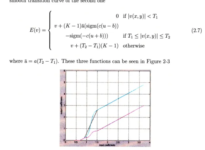
Using these two functions as our basis, in order to accomplish our nonlinear gain, we designed the following function which has the gain factor of the first one and smooth transition curve of the second one

0 if |v(x,y)l < Ti v + (K - 1)a(sigm(c(u - b)) -sigm(-c(u + b)))

v + (T

- T)(K - 1)

(2.7)

where a = a(T2- T1). These three functions can be seen in Figure 2-3

Figure 2-3: Enhancement Functions. Cyan curve: E(v)

Black curve: El(v), Magenta curve:

It was found that if the wavelet coefficients in different directions are treated sep-arately, a coefficient in one direction may be enhanced more than a coefficient in the other direction, creating orientation distortions [13]. Thus, it was decided to find

a value to compare with the thresholds using a combination of our coefficients in different directions in a level. Since orthogonal wavelets were used, the coefficients found for horizontal, vertical, and diagonal components were mapped into orthogonal directions in wavelet domain; therefore, they can be thought as vectors lying orthog-onal to each other in the space, and magnitude of their vector sum can be used as a comparison value. After the denoising and nonlinear enhancement, by recalling the contribution ratios from each component, the enhanced value of the vector sum can be easily transformed back to its three components.

In this way the ratio of the direction components were preserved as well as their weights for computation of the threshold values, and comparisons between thresh-olds and direction components were achieved with one comparison instead of three. Another way to combine three components together may be to think them as scalar quantities; however, thinking of them as vectors has a more logical basis as described above.

We used the same enhancement function for all levels of the wavelet transforma-tion. It should be noted that because lower levels have the information about finer details and higher levels carries information about large scale features of the signal, change of wavelet coefficients in higher levels affects large scale of the signal; and if large gains are used in these levels, then this may create artifacts over large scales of the signal depending on the mother wavelet. Hence, we used higher gains in lower levels to enhance fine details more and decreased the gain with increasing level.

When we transform the image from wavelet domain back to image domain after the denoising and enhancement process, the range of the brightness values is generally larger than that of the original range. Therefore, the new brightness values must be scaled and saturated in order to keep the values in the original range. This will obviously limit the maximum contrast that can be achieved, and reduce the effect of enhancement. The local extrema of the color components of a local area or the global extrema of the color components over the whole image can be used for this purpose. Each pixel can be considered as a local area, and its color components can be scaled with respect to their maximum and minimum. This scaling operation retains

the hue of the enhanced color components, and our results showed that the hues of independently scaled pixels are similar to the original hue, but colors are brighter and tend to be purer. Since it is desired to have the color information similar to the original, we mainly used this scaling method. When global extremas were used; in addition to scaling, we first saturated the color components of the enhanced pixel values with thresholds defined by the global maximum and minimum of each color component, as the global extrema may include outliers; and after that, scaled the color components of the image with respect to these threshold values. Usage of the global extremas resulted in more drastic color changes than using local values, since the scaling operation is normalization of each color component separately, and as a result, it changes the hue.

Chapter 3

Using Wavelet Enhancement on

Images

An image is a two or three dimensional signal, which can be represented discretely as a multidimensional array. If the image is grey-scale, then it will be represented as a two dimensional array and two dimensional wavelet transform can be implemented in order to find the wavelet coefficients. However, for colored images, the 2-D wavelet transform should be applied on one or more color components separately depending on the colorspace of the image. In this thesis RGB and YUV colorspaces were used for image enhancement.

In YUV colorspace, Y component represents luma (brightness), and U and V are the chrominance components. While working on the YUV colorspace we only im-plemented our enhancement algorithm on brightness component, which is the same as enhancing the grey-scale image, and adding color information on it. The YUV colorspace has the advantage of retaining hue as the color information remains un-changed; however, the difference between the original and processed image is less than the difference between the original and enhanced RGB image.

The components of the RGB colorspace are red, green, and blue color values re-spectively. Hence, in contrast to YUV colorspace, the enhancement of the wavelet coefficients should be implemented for each color component. When each color com-ponent is denoised and enhanced independently, it is obvious that the hue information

of each pixel may be changed. Although it may be thought that this change in hue information is undesirable at first, it should be considered that the received color in-formation from the cameras is affected by the weather and lighting conditions of the environment. Therefore, a change in the hue in a good way is, on the contrary, desir-able. We observed that when the color components were enhanced independently, the result was generally brighter and enhancement favors the dominant color component over the others, resulting a small shift towards purer colors.

The change in color information becomes more obvious as higher levels are en-hanced, since the contrast information in large areas is supplied by the wavelet co-efficients in higher levels. However, we also encountered some problems during our experimentation that, when the level of the transformation is increased, a strong con-trast in one area may also affect another area on the image, changing its brightness and hue and creating contrast, although there is no strong contrast originally. This can be prevented by choosing smaller gains in higher levels, and using mother wavelets with shorter support functions. The same problem may appear for finer details, but these are generally compensated by the enhancement in higher levels.

Since the wavelet transform is a local transform, denoising and enhancement by wavelets can be implemented on one or more image segments as well as the whole image. For night-time images, the camera noise is higher than in daylight due to lighting conditions, so wavelet denoising can be used as a preprocessing tool in order to get better images. On foggy or hazy days, the features of the objects and obstacles cannot be detected by the driver or the detection algorithms, causing dangerous situations. In the case of fog or haze, emphasis of these features can be achieved by wavelet enhancement.

For our application, we are mostly dealing with cases where detection is possible, and we need to draw the driver's attention to the potentially dangerous objects. However, the detection results are not 100% reliable and misdetections may occur, and we should avoid emphasizing these possible false positives in the image too much. This is a limiting factor for our application, and we should not make the enhancement results too obvious to the end user. A solution for this limitation can be that, if the

detection algorithm also supplies the information about the reliability of the detection, then the enhancement rate can be set higher with increasing reliability.

On the real road conditions, the possible dangerous objects appear on the scene for only a short while, and it is necessary to get the driver's attention on the object in that limited amount of time. For this purpose, only enhancing the object segment may not be enough to get the driver's attention; hence, in order to strengthen our enhancement we also decreased the contrast of the background, and in addition added some dynamic effects such as changing the window size, contrast and brightness of the object segment. These dynamical effects were designed to be executed over a time period; we tried different time periods and determined empirically that period of one second for all the dynamic effects works well.

3.1

Image Layout

In this thesis, images from three different cameras that were mounted on the front part of the vehicle were gathered and used to provide a single image to show the driver. These cameras were placed in such a way that they have a good view when the vehicle is at an intersection. The cameras on the left and right were normal cameras which were located to show the left and right side of the road respectively. The one in the middle was a wide angle camera facing the front of the vehicle and supplied a general view of the intersection. For this project, only the views of the left and right cameras were important, hence, for some examples in the thesis, only one of these camera views will be shown.

Since there were three different camera views on the screen, when an object was recognized in only one of the side cameras, a preprocessing before enhancement would be helpful for the driver to recognize from which side a vehicle was coming. A simple preprocessing is darkening the camera views when there are no potentially dangerous objects and showing the camera views in which dangerous objects were spotted with their original brightness.

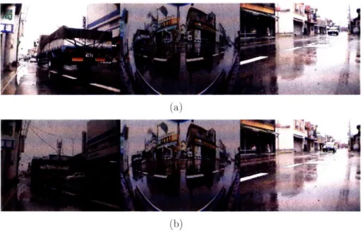
Figure 3-1: Darkening camera views: On (a) the car on the left camera view is detected. However on (b) the car on left view is obscured by the truck, so detection algorithm detects no objects on the left image, and it is darkened.

is a dangerous object or not, by checking the detection results from the last n frames. In order to reduce the latency to switch from dark to bright state, or vice versa, n should be small; but if it is too small, then the reliability decreases. Taking these considerations into account, we designed the decision algorithm such that it changed its state if the check for the reverse state was held for 5 consecutive frames, and stayed in the same state otherwise. The image layout and darkening of the camera views can be seen in Figure 3-1.

3.2

Using Coarse Image Data as the Background

A possible approach to improve the effect of the enhancement is to reduce the contrast of the background that is not detected as a dangerous object. Since 2-D wavelet transform can separate the coarse image data that is stored in the lowpass component from the detailed image data; we can recreate the background image from first or second level coarse images.

The first level coarse image is generally very close to the original, and the objects and most of the details on the image can be identified easily by human eye; therefore,

(a) (b)

(c) (d)

Figure 3-2: Effect of background contrast change: Original image is shown in (a), (b) has the enhanced image on original background, (c) has the enhanced image on first level coarse background, (d) has the enhanced image on second level coarse background

it will not create an important problem for the driver, if there is an undetected object on the background. The second level coarse image loses most of the contrast information, and creates a blurred image, but its additive effect on enhancement is more than the first level coarse background. Hence, the second level coarse image can also be used as the background if the detection results are reliable. Again, the background level can also be chosen automatically if the reliability of the detection results is known. The additive effects of using coarse images as background can be seen on Figure 3-2.

As a general purpose usage, and if there is no information available about the reliability of the detection, we recommend using first level coarse image as the back-ground. However, since the detection was achieved manually throughout this project, a second level coarse background was generally used in our examples in order to

em-phasize the enhancement results more. It is also assumed that the second level coarse image is used for the background in the following sections.

3.3 Window Size Changes

Humans recognize moving objects more easily than stationary ones; it is because human eye is sensitive to changes. Therefore, an effect which adds to the movement around the target object, increases the probability of the driver noticing that object in the image. A way of creating this effect is to change the size of the enhancement window on which we are implementing denoising and enhancement algorithms.

When the dangerous object is far away, due to perspective projection, both the object and the movement of the object on the image is rather small. This makes it hard for the driver to perceive the object. However, when the object is large, the necessity of the window size changes is small. Therefore, we determined a threshold to activate the window size changes; when it was smaller than a certain threshold, it was active, but inactive otherwise. Since the size of the object depends on the overall image size, the threshold was determined as 20% of the minimum of height and width of the image for both height and width of the object. The maximum size change is also determined as 20% of the minimum of height and width of the image, in the same manner.

A possible problem that may occur during change of window size is that, part of the range of the expanded window may be outside the image area. This problem can simply be solved by checking the coordinates of the window, and choosing the area inside the image, or placing the window inside the image by not changing its size but its position.

If the size of the window changes from its original size to the maximum size in consecutive frames, this may distract the driver; hence, it is better to change the size of the segment windows gradually. With this idea on mind, we applied five different window size changes. The first one was to expand the window size from its original to the maximum over a certain period. The second one was to shrink the window

size from its maximum to its original, which can be thought as reverse of the first one. It may also be desired to use the window size changes over half period and keep the window at its maximum or minimum over the rest of the period, and this idea was also applied as the other two effects. The last window size change effect was a combination of the first and the second ones, which is to expand the window size over the first half of the period and shrink it over the second half.

Other kind of size changes may be expanding the window height while shrink-ing the width or vice versa. However, these kind of changes created a movement impression less effective than the ones that were described above; hence, these were not included in the final stage of the project. The window size changes are defined mathematically in equation (3.1)

s = s + k * emax (3.1)

where s is height or width of the segment, emax is the maximum enlargement in terms of pixels, and k is the multiplication factor which is differs for each window size change, and can be defined in (3.2-3.6) respectively

k = (mod(n, T))/T (3.2) k = mod(-n, T)/T (3.3) 2mod(n, T)/T if mod(n, T) < T/2 k -(3.4) 1 if mod(n, T) > T/2

f

k = 1 - 2(T/2 - IT/2 - mod(n - 1, T)I)/T (3.6)

where mod(a, b) is the smallest non-negative integer which is congruent to a modulo

b.

Once people recognize an object in the scene while driving, they will keep in mind that the object is there and may be dangerous. Therefore, it is of extra importance that when a new object is first detected by the detection algorithm. In most of these

cases, if the object was not obscured by another, the object was small and it appeared to be moving slowly, as we discussed before in this section. Because of these, a strong and easily recognizable effect which can be enabled or disabled by the driver was designed when an object was first detected, a window which shrinks from the whole camera image to the object segment over a period. We also used saturation and scaling with respect to the maximum and minimum of color values over the whole enhanced segment instead of scaling the brightness values independently for each pixel, which resulted in color changes on a greater scale as stated above. However, since the effect period is small, the driver may not be able to catch the first time, hence it is better to execute this strong effect more than once; but as the objects appear on the image generally for several seconds, execution of this effect too many times is unnecessary and should be avoided; hence executing it 2-3 times is a good compromise.

3.4

Contrast Changes

The idea behind changing contrast over a period is the same as changing window size; to increase the possibility of recognition by the driver by creating a change over a period of time. We can change the contrast rate of the image by a simple image morphing technique, using a percentage of the brightness values of the enhanced image and a percentage of brightness values of the background which is the second level coarse image as it was stated in section 3.2, with a total of 100%.

We followed an approach, similar to window size changes, for contrast changes. The transition between the enhanced image and the background was achieved by gradual changes, and the ratio between the enhanced image and background was defined with a multiplication factor which was determined by the period and how long the object was detected in the image. However, we have not limited the execution of this effect by the size of the segment as we did for window size changes; instead, this effect was executed unless the obstacle was first detected and the corresponding window size change effect that we discussed in section 3.3 was performing.

As in the case of window size changes, several different contrast change effects can be designed. In this thesis, five different contrast changes which were actually analogous to window size changes were designed. The first two effects were to change the contrast of the image segment from the coarse to the enhanced image, and from the enhanced to the coarse image during one period. The third and fourth effects were to increase the contrast of the segment from coarse to enhanced or decrease it from enhanced to coarse over half period and hold the enhanced image segment for the other half period. These two effects may be desirable over the first two since there would be a, change in the image segments in which objects were located and also the difference between the background and these segments would be large enough to detect for most of the period. The last contrast change effect, which was a combination of first two as in the case of window size change effects, was increasing the contrast of the image segments from coarse to enhanced for the first half period and decreasing it back in the second half. The general formulation for contrast changes can be defined as in

(3.7)

b(x, y) = kl * k * m(x, y) + ( - ki * k) * n(x, y) (3.7) where k is the multiplication factor, ki is a value in [0, 1] which defines the range of contrast change, b(x, y) is the resulting brightness, n(x, y) is the enhanced brightness, and m(x, y) is the background brightness of three color components of a pixel in the image segment. Since there is an analogy between the window size changes and contrast changes, k can be found from (3.2-3.6) respectively.

The contrast change effects and window size change effects can be classified in two separate groups, since they create different kinds of dynamical effects in the image segment, and they can be used together. Therefore, these two categories of effects were implemented in such a way that a driver can choose an effect from each class, or just choose one effect from either of them and none from the other one. However, the choice of effect is global, i.e. it is the same for every detected object in the image.

3.5

Other Dynamic Effects

Other than the window size changes and the contrast changes, other dynamic effects can be found in order to be used for creating a change in image segments to draw driver's attention. Moving the window around the image segment or changing the segment's brightness are examples that were used in this thesis. Enlarging the image segment was also considered but we decided not to use it due to problems that will be discussed in the rest of this section.

The enhancement window can be placed in the image relative to an image seg-ment of object, and can be translated in a defined way over a period to create a movement impression. This movement can be a vibration in the vertical or the hori-zontal direction or both. However, vibrations may create a wrong impression about the movement of the object in the segment; it may seem to be going faster or slower than it really is, which can be risky. Another way to move the enhancement window around the object is to translate it in a circular fashion, either clockwise or counter-clockwise. This movement can be defined by two multiplication factors, and should be defined for starting and ending pixels rather than just the width or height of the segment as in (3.8) and (3.9)

Xmin : Xmini + [emax * ki] (3.8)

Xmaxi = Xmin + Si (3.9)

where Xmini are the original starting points, Xmini and Xmaxi are the resulting starting

and ending points of the segment respectively, ki _{are the multiplication factors, emax}

is the maximum enlargement in terms of pixels, si are either height or width of the segment, and the index i defines the vertical or horizontal direction. k1 and k2can

be defined as 4mod(n, T/4)/T if mod(n, T) < T/4 1 if T/4 < mod(n, T) < T/2 kl= -(3.10) 1 - 4mod(n, T/4)/T if T/2 < mod(n, T) < 3T/4 0 if 3T/4 < mod(n, T) < T 0 if mod(n, T) _ T/4 4mod(n, T/4)/T if T/4 < mod(n, T) • T/2

k2

=

(3.11)

Since this kind of change is close to window size changes, and cannot be used at the same time; hence, it was included in the same category with the window size changes.

Similar to changing the segment contrast over a period, brightness of the image can also be changed in the same manner. The only difference between them is using '0' as the brightness, i.e. a black pixel, instead of using the brightness value of the background. Hence, the brightness changes can also be implemented using (3.7) and the multiplication factors in (3.2-3.6). However, if kI is chosen close to 1, then in some frames the brightness of the resulting segment becomes too low for the human eye to see the object; and if it is close to 0, then there will only be a small brightness change; hence, we recommend the range of k1 as [0.4,0.6]. Since contrast and brightness

change effects are similar, they can also be included in the same category with contrast changes.

The image segments of the objects can also be enlarged via wavelet transform by using the methods in [3] or [22] in order to create a zooming effect, and can be placed in the image. However, while placing the enlarged image segment, two problems will be encountered. First, there will be discontinuities between the background and the segment due to the size change. It should be noted that the resulting discontinuities will not be very clear when the background is coarse; and therefore will be hard to be recognized. Even if the original background is chosen, a transition region can be formed around the enlarged segment and a smooth transition which will not disturb

human eye will be achieved. The second and more important problem is to decide where to place the enlarged segment. If it is placed in the image by centering the original segment, the additive translation vector of the objects will be towards the camera they are captured, due to the perspective projection. This will create a wrong impression about the object's movement. This problem can be understood better by looking at Figures 3-3 and 3-4. In Figure 3-3, assume that vehicle Vo follows a linear trajectory 11; in that case it reaches its twice height and width in the image when it is in the place of vehicle Vr. However, if the enlarged object is placed centering the segment of Vo in the image, then driver will have the impression that the object is in the place of Vp. The same case occurs for the following frames; in Figure 3-4, when a vehicle is following a linear trajectory k1, it can be at points 1, 2, 3, 3-4, 5 in the consecutive frames, while the enlarged segments will give the impression that the observed vehicle is at points 1', 2', 3', 4', 5' respectively, which are on a parallel line k2. Therefore, the driver will have the impression that the observed vehicle is following trajectory k2. One solution for this problem is to foretell where the object will be when it receives the size of the enlarged segment on the camera view originally, and this may be achieved by prediction techniques like Kalman Filter.

However, prediction methods have not been studied in this thesis.

Figure 3-3: Problem with the perspective projection when the object is enlarged. Vehicle Vo will receive its twice size in the image when it is in the place of vehicle Vr. When the enlarged segment of Vo is placed by centering the original segment, it will

be perceived as if it is in the place of vehicle Vp.

Figure 3-4: A vehicle following the trajectory ki will be perceived as if it is follow-ing the trajectory k2, when its enlarged segment is placed by centerfollow-ing the original segment.

Chapter 4

Experimental Results

The results shown in this chapter were found by using symlet-6

mother wavelet whose scaling and wavelet functions are shown in Figure 4-1, and

wavelet denoising and enhancement were implemented for 5 levels of wavelet transform.

The original images are composed of three 240x320 pixel images from three cameras,

and generally only one of these camera views were shown in the figures. In

the images where only the segment was enhanced, the second level background was used, since

the segmentation was achieved manually as it was stated in section 3.2.

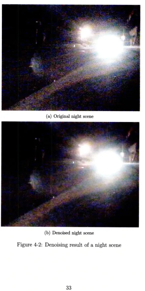
A wavelet denoising result was shown in a night-time image which

has high noise. Since the noise component cannot be totally eliminated; when night-time

scenes were also enhanced, the resulting images will still be noisy. As a result,

enhancement makes these images worse, since it also amplifies the remaining noise component.

Hence,

(a) scaling function (b) wavelet function Figure 4-1: Scaling and wavelet functions of sym-6

it was decided that only denoising will be used for night-time images. However, if a better quality camera is used, and the noise component is lower, then the enhancement can also be implemented. An example of a night image is given in Figure 4-2.

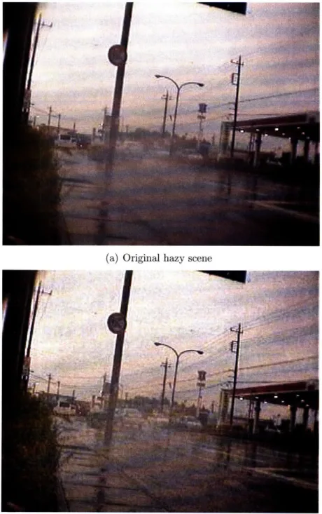
Enhancement of full camera view can be used for foggy or hazy scenes as it was stated in chapter 3. Again, it should be stated that in foggy and hazy scenes, fine details make the image more visible, so high gain values should be used especially for first two levels. Although high frequency noise is increased due to the large enhancement gains, it is tolerable since it increases the visibility which is crucial for these conditions. In Figure 4-3 enhancement of whole camera view from a hazy scene is shown.

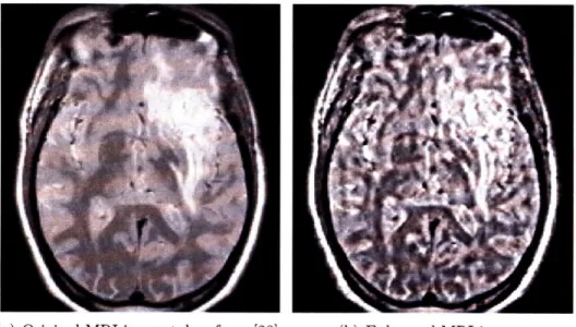
The effect of enhancement can be recognized well when it is applied on low-contrast images. Although the application field is out of topic of this thesis; an enhancement example is shown in Figure 4-4 in an MRI image taken from [23], since it will give a better understanding of our image enhancement technique.

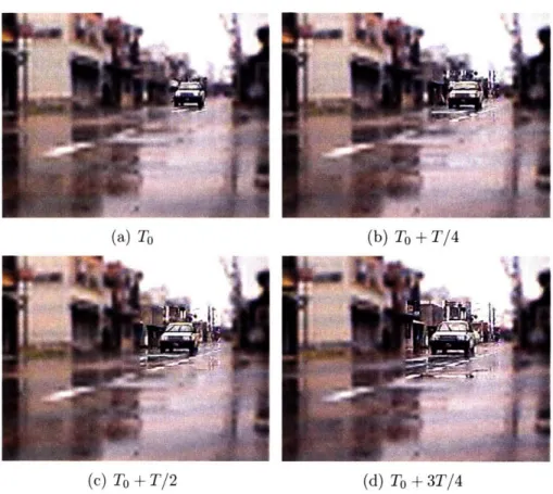
The enhancement of a segment of an image is shown following in this chapter, with contrast and window size changes added; however, since these effects need more than one picture to be understood, the camera views of captured frames at four different times i.e. the beginning of the period, one quarter of the period, half period, and three quarters of the period are shown in order to give the impression of each effect in the following figures.

(a) Original night scene

(b) Denoised night scene

(a) Original hazy scene

(b) Enhanced hazy scene

(a) Original MRI image taken from [23]

Figure 4-4: Enhancement result of an MRI image.

(a) To _{(b) To + T/4}

(c) To + T/2 (d) To + 3T/4

Figure 4-5: Original image sequence

(a) To (b) To + T/4

(c) To + T/2 (d) To + 3T/4

Figure 4-6: Expanding window size

(a) To (b) To + T/4

(c) To + T/2 (d) To + 3T/4

(a) To (b) To + T/4

(c) To + T/2 (d) To + 3T/4

Figure 4-8: Increasing contrast

(a) To (b) To + T/4

(c) To + T/2 (d) To + 3T/4

(a) To (b) To + T/4

(c) To + T/2 (d) To + 3T/4

Figure 4-10: Moving window

(a) To (b) To + T/4

(c) To + T/2 (d) To + 3T/4

Chapter 5

Conclusion

5.1

Conclusion

In this thesis, image enhancement techniques based on wavelet transform were ex-plored. The image regions in which potentially dangerous vehicles were located were denoised and enhanced using the coefficients in vertical, horizontal, and diagonal di-rections in the wavelet domain. First, based on a decision algorithm, the camera views without potentially dangerous vehicles were darkened relative to those views with potentially dangerous vehicles, in order to give the driver an idea about which direction a vehicle is approaching. Both soft and hard thresholding techniques were used for denoising in different levels of the transform, and a non-linear function was found for enhancement. A smoothed background was used to increase the effect of the enhancement. In addition, dynamic effects such as changing the size or the location of the segment window, and the contrast or the brightness of the segments with time were implemented in order to make vehicles more noticeable.

The results showed that when coarse image is used as the background, the differ-ence in contrast between the background and the image segment is high enough to make objects noticeable. The dynamical effects also increased the detectability of the objects.

5.2

Future Work

We propose the following extensions for this research:

1. The threshold values and enhancement gains can be adjusted for each driver through supervised learning for different weather and lighting conditions.

2. Movement of the objects can be estimated and corresponding object location can be predicted by a prediction algorithm, hence use of the enlarged image segments will be enabled.

Bibliography

[1] A. Boggess and F. J. Narcowich. A First Course in Wavelets with Fourier

Anal-ysis. Prentice-Hall, January 2001.

[2] A. V. Bronnikov and G. Duifhuis. Wavelet-based image enhancement in x-ray imaging and tomography. Appl. Opt., 37(20):4437-4448, July 1998.

[3] S. G. Chang, Z. Cvetkovid and M. Vetterli. Resolution enhancement of images using wavelet transform extrema interpolation. In Proceedings ICASSP-95 (IEEE

International Conference on Acoustics, Speech and Signal Processing), volume 4,

pages 2379-2382, Detroit, MI, USA, 1995.

[4] S. G. Chang, B Yu and M. Vetterli. Adaptive wavelet thresholding for image denoising and compression. IEEE Transactions on Image Processing,

9(9):1532-1546, September 2000.

[5] I. Daubechies. Ten Lectures on Wavelets. Society for Industrial and Applied Mathematics, Philadelphia, PA, USA, 1992.

[6] E. Dickmanns. The development of machine vision for road vehicles in the last decade. IEEE Intelligent Vehicles Symposium, 1:268-281, June 2002.

[7] D. L. Donoho. De-noising by soft-thresholding. IEEE Transactions on

Informa-tion Theory, 41(3):613-627, May 1995.

[8] D. L. Donoho and I. M. Johnstone. Ideal spatial adaptation by wavelet shrinkage.

[9] D. M. Gavrila, J. Giebel and S. Munder. Vision-based pedestrian detection: The protector system. IEEE Intelligent Vehicles Symposium, pages 13-18, June 2004. [10] A. Graps. An introduction to wavelets. IEEE Computer Science and Engineering,

2(2):50-61, June 1995.

[11] U. Handmann, T. Kalinke, C. Tzomakas, M. Werner, and W. von Seelen. An image processing system for driver assistance. In IV'98, IEEE International

Conference on Intelligent Vehicles, pages 481-486, Stuttgart, Germany, 1998.

IEEE.

[12] D. J. Jobson, R. Zia-ur and G. A. Glenn. A multiscale retinex for bridging the gap between color images and the human observation of scenes. IEEE Transactions

on Image Processing, 6(7):965-976, July 1997.

[13] A. Laine, J. Fan and W. Yang. Wavelets for contrast enhancement of digital mammography. IEEE Engineering in Medicine and Biology Magazine, 14(5):536-550, September/October 1995.

[14] J. M. Lina and L. Gagnon. Image enhancements with symmetric daubechies wavelets. Wavelet Applications in Signal and Image Processing III, Proceedings

of SPIE, (2569):196-208, 1995.

[15] J. Lu, D. M. Healy and J. B. Weaver. Contrast enhancement of medical images using multiscale edge representation. In H. H. Szu, editor, Proceedings of SPIE, volume 2242, pages 711-719, March 1994.

[16] S. G. Mallat. A theory for multiresolution signal decomposition: The wavelet rep-resentation. IEEE Transactions on Pattern Analysis and Machine Intelligence,

11(7):674-693, July 1989.

[17] H. L. Resnikoff and R. O. Wells, Jr. Wavelet Analysis: The Scalable Structure

[18] P. Sakellaropoulos, L. Costaridou and G. Panayiotakis A wavelet-based spatially adaptive method for mammographic contrast enhancement. Physics in Medicine

and Biology, 48(6):787-803, 2003.

[19] J.-L. Starck, F. Murtagh, E. Candes and D. L. Donoho. Gray and color image contrast enhancement by the curvelet transform. IEEE Transactions on Image

Processing, 12(6):706-717, June 2003.

[20] Z. Sun, G. Bebis and R. Miller. On-road vehicle detection: A review. IEEE

Transactions on Pattern Analysis and Machine Intelligence, 28(5):694-711, May

2006.

[21] Y. Y. Tang, J. Liu, L. Yang, and H. Ma. Wavelet Theory and Its Application to

Pattern Recognition, volume 36 of Series in Machine Perception and Artificial Intelligence. World Scientific, March 2000.

[22] A. Temizel and T. Vlachos. Image resolution upscaling in the wavelet domain us-ing directional cycle spinnus-ing. SPIE Journal of Electronic Imagus-ing, 14(4):040501, Oct.-Dec. 2005.

[23] X. Zong, A. F. Laine., E. A. Geiser and D. C. Wilson. De-noising and con-trast enhancement via wavelet shrinkage and nonlinear adaptive gain. Wavelet