HAL Id: insu-02133870
https://hal-insu.archives-ouvertes.fr/insu-02133870
Submitted on 17 Oct 2019
HAL is a multi-disciplinary open access
archive for the deposit and dissemination of
sci-entific research documents, whether they are
pub-lished or not. The documents may come from
teaching and research institutions in France or
abroad, or from public or private research centers.
L’archive ouverte pluridisciplinaire HAL, est
destinée au dépôt et à la diffusion de documents
scientifiques de niveau recherche, publiés ou non,
émanant des établissements d’enseignement et de
recherche français ou étrangers, des laboratoires
publics ou privés.
wind-adjusted superresolution
Lieven Clarisse, Martin van Damme, Cathy Clerbaux, Pierre-François Coheur
To cite this version:
Lieven Clarisse, Martin van Damme, Cathy Clerbaux, Pierre-François Coheur. Tracking down global
NH3 point sources with wind-adjusted superresolution. Atmospheric Measurement Techniques,
Euro-pean Geosciences Union, 2019, 12 (10), pp.5457-5473. �10.5194/amt-12-5457-2019�. �insu-02133870�
https://doi.org/10.5194/amt-12-5457-2019 © Author(s) 2019. This work is distributed under the Creative Commons Attribution 4.0 License.
Tracking down global NH
3
point sources with
wind-adjusted superresolution
Lieven Clarisse1, Martin Van Damme1, Cathy Clerbaux2,1, and Pierre-François Coheur1
1Atmospheric Spectroscopy, Service de Chimie Quantique
et Photophysique, Université libre de Bruxelles (ULB), Brussels, Belgium
2LATMOS/IPSL, Sorbonne Université, UVSQ, CNRS, Paris, France
Correspondence: Lieven Clarisse (lclariss@ulb.ac.be)
Received: 13 March 2019 – Discussion started: 20 May 2019
Revised: 17 July 2019 – Accepted: 15 September 2019 – Published: 17 October 2019
Abstract. As a precursor of atmospheric aerosols, ammonia (NH3) is one of the primary gaseous air pollutants. Given its
short atmospheric lifetime, ambient NH3concentrations are
dominated by local sources. In a recent study, Van Damme et al. (2018) have highlighted the importance of NH3point
sources, especially those associated with feedlots and indus-trial ammonia production. Their emissions were shown to be largely underestimated in bottom-up emission inventories. The discovery was made possible thanks to the use of over-sampling techniques applied to 9 years of global daily IASI NH3satellite measurements. Oversampling allows one to
in-crease the spatial resolution of averaged satellite data beyond what the satellites natively offer. Here we apply for the first time superresolution techniques, which are commonplace in many fields that rely on imaging, to measurements of an at-mospheric sounder, whose images consist of just single pix-els. We demonstrate the principle on synthetic data and on IASI measurements of a surface parameter. Superresolution is a priori less suitable to be applied on measurements of vari-able atmospheric constituents, in particular those affected by transport. However, by first applying the wind-rotation tech-nique, which was introduced in the study of other primary pollutants, superresolution becomes highly effective in map-ping NH3 at a very high spatial resolution. We show that
plume transport can be revealed in greater detail than what was previously thought to be possible. Next, using this wind-adjusted superresolution technique, we introduce a new type of NH3map that allows tracking down point sources more
easily than the regular oversampled average. On a subset of known emitters, the source could be located within a median distance of 1.5 km. We subsequently present a new global
point-source catalog consisting of more than 500 localized and categorized point sources. Compared to our previous cat-alog, the number of identified sources more than doubled. In addition, we refined the classification of industries into five categories – fertilizer, coking, soda ash, geothermal and ex-plosives industries – and introduced a new urban category for isolated NH3hotspots over cities. The latter mainly
con-sists of African megacities, as clear isolation of such urban hotspots is almost never possible elsewhere due to the pres-ence of a diffuse background with higher concentrations. The techniques presented in this paper can most likely be ex-ploited in the study of point sources of other short-lived at-mospheric pollutants such as SO2and NO2.
1 Introduction
As one of the primary forms of reactive nitrogen, NH3is
es-sential in many of the Earth’s biogeochemical processes. It is naturally present along with the nitrogen oxides in the global nitrogen cycle (Canfield et al., 2010; Fowler et al., 2013). However, the discovery of ammonia synthesis through the Haber–Bosch process in the early 1900s has made this vi-tal compound available in almost unlimited quantities, sup-porting the explosive population growth in the last century (Erisman et al., 2008). As a result, the nitrogen cycle is cur-rently perturbed beyond the safe operating space for human-ity, which has led to a host of environmental and societal problems (Steffen et al., 2015). The most obvious direct im-pact of excess NH3is that on air quality, as atmospheric NH3
mat-ter, which has important adverse health impacts (Lelieveld et al., 2015; Bauer et al., 2016). Emissions of the two other important precursors (SO2and NOx), thanks to effective
leg-islation, drastically decreased in the past 20 years in Europe and North America and have started to level off in eastern Asia (Aas et al., 2019; Georgoulias et al., 2019). In contrast, no such decreases are observed or expected in the near fu-ture for NH3(e.g., Warner et al., 2017; Sutton et al., 2013).
Unlike the other precursors, NH3emissions are not well
reg-ulated, and in fact, the focus on decreasing NOxand SO2has
already led to increased NH3emissions (Chang et al., 2016)
and concentrations (Lachatre et al., 2018; Liu et al., 2018). The lack of a global regulative framework stems in part from the historical relative difficulty in measuring NH3
con-centrations. Satellite-based measurements of NH3, which
were discovered about a decade ago, offer an attractive com-plementary means of monitoring NH3. Satellite datasets have
now reached sufficient maturity to be directly exploitable, even when the individual measurements come with large and variable uncertainties. Using satellite observations we have recently shown the importance of ammonia point sources on regional scales (Van Damme et al., 2018). In total, over 240 of the world’s strongest point sources were identified, cate-gorized and quantified. Somewhat expectedly, many of these point sources (or clusters thereof) were found to be associ-ated with “concentrassoci-ated animal feeding operations” (CAFOs; Zhu et al., 2015; Yuan et al., 2017). However, much more sur-prisingly was the number of identified industrial emitters and in particular those associated with ammonia and urea-based fertilizer production. An evaluation of the EDGAR inven-tory additionally showed that emission inventories vastly un-derestimate the majority of all point-source emissions, even when a conservative average NH3lifetime of 12 h is assumed
in the calculation of the satellite-derived fluxes. Industrial processes could therefore be extremely important, especially on a regional scale. Altogether, these findings were made possible due to the availability of the large multiyear NH3
dataset (Whitburn et al., 2016; Van Damme et al., 2017) de-rived from measurements of the IASI spaceborne instrument (Clerbaux et al., 2009) and the oversampling technique that was applied to sufficiently resolve localized emitters.
Oversampling techniques applied on measurements of satellite sounders allow obtaining average distributions of at-mospheric constituents at a higher spatial resolution than the original measurements (Sun et al., 2018). They exploit the fact that the footprint on the ground of satellite measure-ments varies in location, size and shape each time the satel-lite samples an area. When pixels partially overlap, some information becomes available on their (subpixel) intersec-tion. High-resolution mapping can, however, only be ob-tained by combining typically many hundreds of measure-ments. A crucial condition on which oversampling relies is that the pixel center and ground instantaneous field of view (GIFOV) of satellite measurements is known with a high ac-curacy (typically < 1 km, as opposed to the coarse spatial
resolution of the extent of the satellite pixel, which is typ-ically > 10 km). Practical implementation of oversampling is relatively straightforward once the footprint is known: a fine subgrid is constructed in which the value of each cell of the grid is obtained as the average value of all overlapping GIFOVs. Optionally, the averaging can be weighted to take into account measurement error, total pixel surface area and spatial response function. We refer to Sun et al. (2018) and Van Damme et al. (2018) for comprehensive reference mate-rial on averaging and oversampling, detailed algorithmic de-scriptions, and practical considerations for their implementa-tion.
Oversampling has gradually become commonplace in the field of atmospheric remote sensing, especially in the study of short-lived pollutants such as NO2 (Wenig et al., 2008;
Russell et al., 2010), SO2 (Fioletov et al., 2011, 2013),
HCHO (Zhu et al., 2014) and NH3 (Van Damme et al.,
2014, 2018). The increased spatial resolution enables in the first instance a much better identification of emission (point) sources, quantification of their emissions (Streets et al., 2013), and study of transport and plume chemistry (de Foy et al., 2009). Oversampling applied to the study of point sources becomes even more useful when wind fields are taken into account. Beirle et al. (2011) showed that binned averaging per wind direction allows simultaneous estimates of both emission strengths and atmospheric residence times. Valin et al. (2013) and Pommier et al. (2013) introduced the wind-rotation technique whereby each observation is rotated around the presumed point source according to the horizon-tal wind direction, effectively yielding a distribution in which the winds blow in the same direction. As we will also demon-strate (see Sect. 3), this reduces the overall spread of the transported pollutants and reduces contributions of nearby sources. Combining plume rotation with oversampling has proven to be a very successful technique for the study of NO2and SO2point sources, leading to massively improved
inventories and emission estimates and better constraints on the atmospheric lifetime of these pollutants (Fioletov et al., 2015, 2016, 2017; Wang et al., 2015; de Foy et al., 2015; Lu et al., 2015; Liu et al., 2016; McLinden et al., 2016).
However, as pointed out in Sun et al. (2018), while over-sampling offers an increased resolution, it still yields a smoothed representation of the true distributions. There ex-ists a large field of research, collectively referred to as super-resolution (Milanfar, 2010), that attempts to construct high-resolution images from several possibly moving or distorted low-resolution representations of the same reality. Oversam-pling is in essence the simplest way of performing superres-olution but in a way that does not fully exploit the spatial information of the measurements. Superresolution has been applied before in the field of remote sensing of land or land cover (e.g., Boucher et al., 2008; Xu et al., 2017), but even though it is theoretically possible, it has not been applied to atmospheric-sounding measurements. In this case, the “im-ages”, as taken by sounders, are of the lowest resolution; i.e.,
they correspond to single, uniformly colored pixels. Perhaps the main reason why superresolution has not been attempted before on atmospheric sounders is that these rely on the fact that the low-resolution samples should be derived from an underlying distribution that does not change in time (de Foy et al., 2009). When this is not the case, the smoothing in-troduced by oversampling is actually desirable. With the ar-rival of the wind-rotation technique, most of the variabil-ity observed for point-source emitters can be corrected for, and therefore superresolution becomes viable for short-lived species as NH3.
In Sect. 2 we introduce superresolution and demonstrate its effectiveness on measurements of the IASI sounder for a parameter related to (constant) surface emissivity. Next we illustrate the application of what we coin “wind-adjusted supersampling” on an industrial point source of NH3. In
Sect. 3 we use ideas from McLinden et al. (2016) to pro-vide a new type of NH3map, one that is supersampled and
wind-corrected at the same time. This map enables the iden-tification of many new point sources in addition to the ones reported in Van Damme et al. (2018). We performed a de-tailed global analysis of this new map, which led to the iden-tification and categorization of more than 500 point sources and which we present in Sect. 4.
2 Superresolved oversampling
The general superresolution problem does not have a unique solution, as the available low-resolution measurements typ-ically do not hold all the required information content (i.e., the problem is underdetermined). It is usually also overde-termined because of measurement noise and, for our case es-pecially, because of temporal variability. As a consequence, there is no unique best algorithm, and a myriad of alternatives exist. For this study, we chose the iterative back-projection (IBP) algorithm (Irani and Peleg, 1993), as it takes a partic-ular intuitive and simple form for single-pixel satellite ob-servations and allows addressing the ill-determined nature of the problem. It proceeds as follows. Suppose we have a set of single-pixel measurements M0 of a spatially
vari-able quantity. For the first iteration, the solution of the al-gorithm corresponds to the regular oversampling, which we will write as SS1=OS1=OS(M0)(SSi stands for the
so-lution of the supersampling obtained in iteration i, and OS stands for the oversampling operator). From this oversam-pled average, we then calculate simulated observations for each of the original individual observations, corresponding to what the instrument would see if the ground truth were SS1.
The entire set of these simulated measurements will be de-noted by M1=M(SS1)(with M the operator that simulates
the measurements). If the oversampled average OS1=SS1
corresponds to the ground truth, then M1would clearly
coin-cide with M0. However, as oversampling typically smooths
out the observations, this is generally not the case. An
im-proved estimate of the average (SS2) can be obtained by
adding OS(M0−M1)to the oversampled average, therefore
correcting (partially) the observed differences. This process then is repeated to obtain increasingly better estimates. The entire algorithm thus reads
SS1=OS(M0) =OS1 →M1=M(SS1), (1) SS2=SS1+OS(M0−M1) =SS1+OS1−OS2 →M2=M(SS2), (2) .. . SSk=SSk−1+OS (M0−Mk−1) =SSk−1+OS1−OSk →Mk=M(SSk). (3)
The solution converges to an average that is maximally con-sistent with the observations, i.e., M0≈Mk for sufficiently
large k (as shown in Elad and Feuer, 1997, IBP converges to the maximum likelihood estimate whereby M0−Mkis
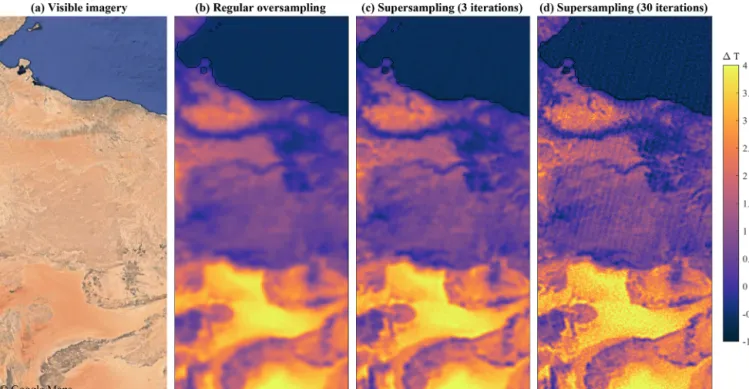
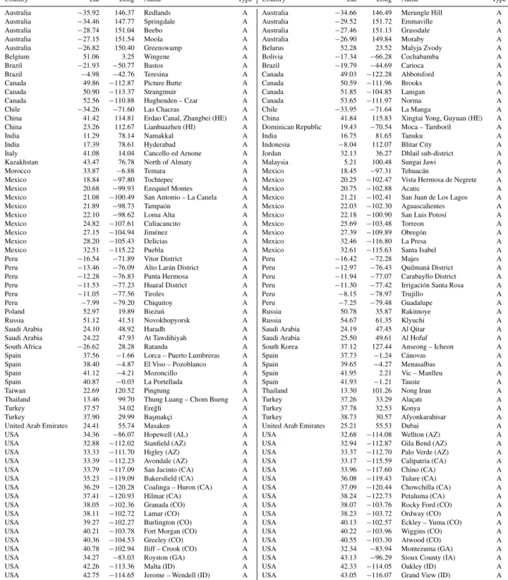
min-imized). Figure 1 illustrates the algorithm on synthetic data with an idealized ground truth made up of nine point sources (Fig. 1a), with a Gaussian spread between 0.5 and 40 pix-els. The measurement footprint was assumed to be variable between 7 and 13 pixels. The SS1 (Fig. 1b), SS3 (Fig. 1c)
and SS50 (Fig. 1d) averages illustrate the convergence and
strengths of the algorithm well, which reproduces most of the point sources near perfectly and even partly resolves the smallest feature (compare also with Sun et al., 2018, Fig. 8). Some small ringing effects are noticeable though after 50 it-erations (best visible on a screen), which are the result of the undetermined nature of the problem (Dai et al., 2007).
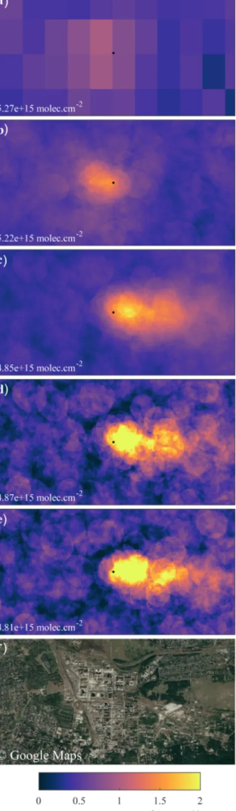
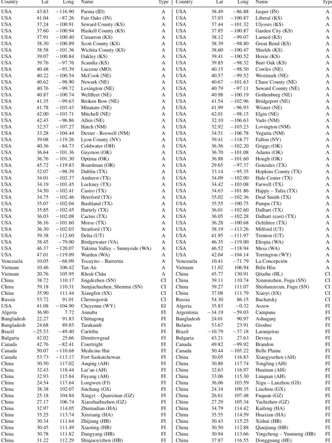
An example applied to real data is shown in Fig. 2, which shows part of the Sahara and Mediterranean Sea. The quan-tity on which the oversampling is applied is the brightness temperature difference (BTD) between the IASI channels at 1157 and 1168 cm−1. This BTD, located in the atmospheric window, is sensitive to the sharp change in surface emissiv-ity due to the presence of quartz (see Takashima and Masuda, 1987, who also illustrate that the relevant feature is not seen in airborne dust). Being related to the surface, it can be as-sumed to be reasonably constant for each overpass of IASI (note that it is not entirely the case: sand dunes do undergo changes over time, and surface emissivities can depend on the viewing angle and can be affected by changes in moist content). Comparison with visible imagery (Fig. 2a) shows, as expected, that the largest BTD values (> 4 K) are associ-ated with the most sandy areas. The other desert areas exhibit widely varying values, and oceans are slightly negative. The oversampled average (Fig. 2b) captures most large features down to about 5 km in size. Recalling that the footprint of IASI is a 12 km diameter circle at nadir, and elongates to an ellipse of up to 20 km×39 km at off-nadir angles, this ex-ample illustrates why oversampling is such a powerful
tech-Figure 1. Illustration of the supersampling technique on synthetic data. Panel (a) depicts an imaginary ground truth, made up of two-dimensional Gaussian distributions, each with a different spread (0.5 to 40 pixels). The rectangles in (a) indicate the assumed footprint size of the measurements, varying between 7 and 13 pixels. Panel (b) shows the results of the common oversampling approach applied to 100 000 measurements scattered randomly over the area. Panels (c, d) provide the results of the supersampling technique after respectively 3 and 50 iterations.
Figure 2. Illustration of the IBP superresolution technique on IASI observations of a BTD sensitive to surface quartz. All cloud-free ob-servations of IASI for the period 2007–2018 were used for the averages. Panel (a) shows the corresponding visible imagery from Google Maps.
nique. However, the additional resolution brought by the su-persampling is clear, even after three iterations. The small-est features that can be distinguished are about 3–4 km (af-ter three i(af-terations; Fig. 2c) and 2–3 km (af(af-ter 30 i(af-terations; Fig. 2d) in diameter. That said, with increasing iterations, ar-tifacts start to appear due to enhancements of noise and the specific sampling of IASI (in particular, stripes parallel to the orbit track become apparent). Such overfitting to the data and a sensitivity to outliers is often seen in maximum likelihood optimizations (Milanfar, 2010). It can therefore be
advanta-geous to stop the algorithm after a few iterations (which can also be required for computational reasons).
3 Wind-adjusted supersampling
In this section we illustrate the previously introduced super-sampling on a wind-rotated NH3 average centered around
a point source. The ammonia plant at Horlivka (Gorlovka), Ukraine, was chosen as a test case. This plant made the news in 2013 because of the major NH3 leak that occurred on
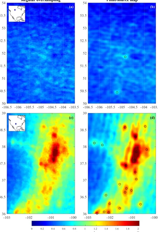
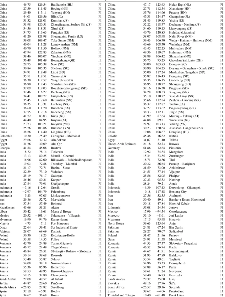
Figure 3. Averaging techniques illustrated on the ammonia plant at Horlivka on IASI NH3data between 2007 and 2013. From top
to bottom: (a) gridded average; (b) oversampled average; (c) wind-rotated oversampling, with the rotation center located at the maxi-mum of (b); (d) wind-rotated supersampling, with the rotation cen-ter located at the maximum of (b); and (e) wind-adjusted supersam-pling around the assumed source (center of the plant). (f) Zoomed-in view (factor of 20) over the ammonia plant (data: © Google Maps). For each subpanel, the number in the bottom left corner is the total average NH3column amount over the entire area.
6 August, killing five people and injuring many more. We refer to the Wikipedia article for a detailed description of the event and a list of related newspaper articles (Wikipedia, 2019). The accident itself was not detected by IASI, but an abrupt drop in the average concentrations after the inci-dent is seen in the satellite observations. In fact, after 2013 NH3 enhancements are no longer detected at or near the
plant. Figure 3 illustrates the processes of oversampling, su-persampling and wind rotation on IASI data from 2007 to 2013. Each subpanel depicts the 120 km×60 km area cen-tered around the plant, from top to bottom.
a. Gridded average. In the regular gridded average, each grid cell is assigned the arithmetic average of all obser-vations whose center falls into the grid cell. This method only gives a faithful representation for larger grid-cell sizes, whereas smaller grid sizes provide a higher res-olution at the cost of larger noise. Here a grid size of 0.15◦×0.15◦was chosen. NH3enhancements are seen
in a wide area around the plant, with a maximum west of the plant of 1 × 10¹⁶molec. cm−2.
b. Oversampled average. Oversampling the daily maps be-fore averaging increases the resolution and reveals the point-source nature of the emission, with a maximum close to the plant (around 1.6 × 10¹⁶molec. cm−2). c. Wind-rotated oversampling. The wind-rotation
tech-nique (Valin et al., 2013; Fioletov et al., 2015) con-sists of rotating the map of daily observations around a presumed point source and along the direction of the wind direction at that point. The rotation was applied here to align the winds in the x direction. Daily hori-zontal wind fields were taken from the ERA5 reanaly-sis (ERA5, 2019) and interpolated at an altitude equal to half of the boundary layer height. The NH3average
shown in this panel was obtained via oversampling ap-plied to all the daily wind-rotated maps. It is important to note that such a distribution can no longer be inter-preted as a geographical map, since each pixel is an average of measurements taken at different places. The only map element that is preserved is the distance to the point source. However, looking at the resulting dis-tribution, the advantages brought by wind rotation are obvious. Whereas in the normal oversampled average the NH3enhancements are scattered across, aligning the
winds significantly enhances both the source and trans-port (with a maximum of 2 × 10¹⁶molec. cm−2). d. Wind-adjusted supersampling (i). The figure in this
panel was obtained from wind-rotated daily maps, as in the previous panel, but this time the average was calculated with three iterations of the IBP supersam-pling algorithm. As explained above, supersamsupersam-pling of-fers most benefits when the underlying distribution can be assumed to be reasonably constant, which is in part
achieved by aligning the winds. The resolution is fur-ther increased, and as the plume is much less smoothed out, maximum observed columns are also much higher (3.3 × 10¹⁶molec. cm−2). Note that in general for NH3,
three iterations of the IBP algorithm seem to offer a good compromise of increasing the resolution of the av-erage without introducing artifacts related to overfitting.
e. Wind-adjusted supersampling (ii). In Fig. 3c and d, the point-source location was taken from Van Damme et al. (2018), where the locations were determined based on the location of the maxima in the oversampled averages. In this last panel, the rotation was applied around the center of the presumed source (the chemical plant). The performance of the wind rotation is further enhanced, yielding a distribution fully consistent with that of a single emitting point source whose emissions undergo transport in a fixed direction. The part of the plume lo-cated furthest from the source is a bit off axis, which is probably caused by inhomogeneities in the wind fields across the entire scene. This panel also illustrates the sensitivity of the rotation method to small shifts in the location of the center, a fact that we will exploit in the next section.
One useful property of the different procedures is that they all approximately conserve the quantity that is being aver-aged; i.e., the averaged quantity in each grid is approximately the same as the average quantity in the grid representing the ground truth given that there is a sufficient number of surements across the entire grid. When the number of mea-surements is low, this can break down dramatically, as can be seen with the extreme example of a single high-value mea-surement over an isolated point source. When a gridded aver-age is made from this single measurement onto a coarse grid (e.g., 5◦×5◦), the entire grid cell containing the measure-ment will be associated with this high value, thus overesti-mating reality. A strict conservation is therefore not possible in general, as not enough information is contained in the orig-inal measurements to reconstruct the ground-truth perfectly even on average. That being said, supersampling conserves quantity with respect to the original measurements, when the number of iterations is large enough. This is a consequence of the fact that the back-projected measurements converge to the actual measurements and therefore also their averages. Finally note that wind rotation does not alter the grid aver-age, as rotation simply redistributes the measurements to dif-ferent locations on the grid. The average total NH3columns
are indicated in each subpanel of Fig. 3. The average of the ungridded measurements within the considered box equals 5.23 × 10¹⁵molec. cm−2. As can be seen, the largest change in the average column is caused by the rotation procedure, but this is simply an artifact caused by limiting the average to a square box around a point source (instead of a circle). This example illustrates that in practice, with differences smaller
than 1 %, the different gridding procedures can be assumed to conserve quantity.
4 An NH3point-source map
Having demonstrated the effectiveness of both the wind-rotation and supersampling approaches in revealing point sources, we are now in a position to introduce a new type of NH3map, specifically designed to track down point sources.
It is based on a similar map presented in McLinden et al. (2016) for SO2, but some important differences were
in-troduced here to make it work for NH3. The main idea of
McLinden et al. (2016) is to treat each location on Earth as a potential point source and to assign it a value propor-tional to the downwind (the source) minus the upwind (the background) column. In particular, for a given location, a wind-rotated average is constructed first, similar to Fig. 3c. Representative average columns are then obtained down-wind and updown-wind from the potential source (e.g., in boxes of 10 km×10 km). Finally, the difference of the upwind and downwind average is calculated, and this value is then used to represent the point-source column at that specific location. While the method works nicely for SO2, this method proved
to be only moderately successful when we applied it to the IASI NH3 data. In particular, for those places where area
sources dominate or where point sources are clustered over too large an area, local variation in the columns produces a noisy map, with many fictitious point sources.
We found that instead of the differences, the downwind average alone produced a more representative point-source map. In addition, applying the method not on the oversam-pled average but on the supersamoversam-pled one allows increas-ing the resolution. There are two key advantages offered by a point-source map constructed in this way as opposed to a regular oversampled average: brighter point sources and smoother (lower) values over the background. The fact that point sources appear brighter is a direct consequence of the plume concentration achieved with wind-rotated supersam-pling, as shown in the previous section. Smoothing of the background is accomplished by the process of averaging the area downwind. However, by applying the method not on an oversampled average but on a supersampled one, this smoothing is partially offset for point sources. The resulting point-source map has a similar horizontal resolution to the oversampled map, but with increased averaged columns at the point sources and a smoother background distribution.
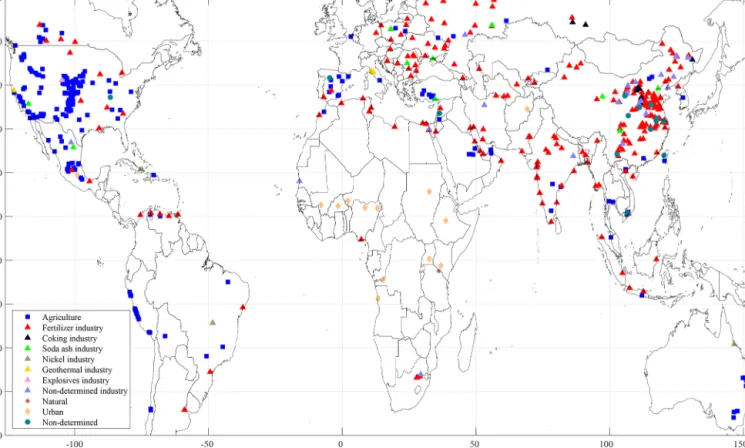
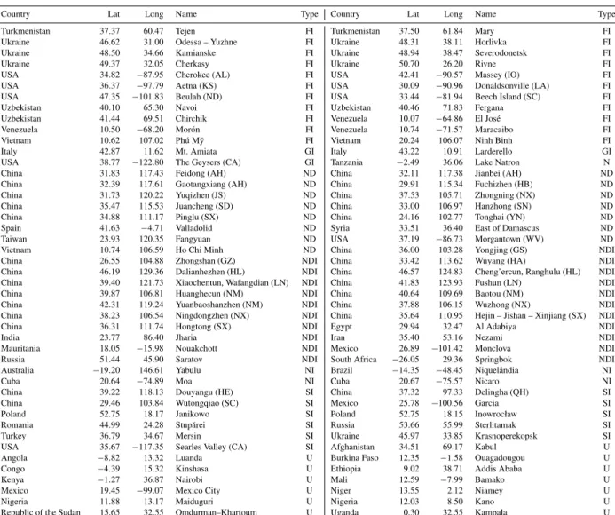
Examples over two selected regions in North America are shown in Fig. 4b and d. In these examples, the downwind av-erages were calculated in boxes extending from −5 to 5 km in the y direction and 0 to 20 km in the x direction. Figure 4a and c correspond to the regular oversampled averages. In Fig. 4a, which shows the oversampled average of the south-ern part of the Saskatchewan province of Canada, no point sources are apparent in the patchy NH3distribution. The
cor-Figure 4. NH3point sources over Canada (a, b) and the US (c, d). Panels (a, c) show maps produced with a regular oversampled average, and panels (b, d) depict the corresponding NH3point-source maps. The black circles indicate the identified point sources.
responding point-source map, shown in Fig. 4, is smoother over areas dominated by the diffuse sources, where column variations are close to the measurement uncertainty. In addi-tion, two bright spots are evident, which upon investigation coincide with the location of an ammonia plant (Belle Plaine) and a very large feedlot (> 2 km in length) near the town of Lanigan. Looking back at the oversampled average, even with the advantage of hindsight, these sources can hardly be
singled out. Figure 4c and d show the southwestern part of Kansas, US. It is an area well known for its cattle (Harring-ton and Lu, 2002). In Van Damme et al. (2018) several point sources associated with feedlots were isolated in Kansas and the rest of the High Plains region, but most of the area was found to be too diffuse to allow identification of individual point sources. The NH3point-source map facilitates greatly
and the fact that the main point sources contrast much more with the background. An added benefit of this is that the lo-cation of the maxima in the map is in general closer to the actual emission source than is the case in the oversampled map, making it easier to track down the suspected source with visible imagery and therefore also to assign and iden-tify the point source.
Displaced maxima that are seen in regular averages (wind-adjusted or not) can also be the result of transport, as noted by Van Damme et al. (2018), who found that especially for coastal sites, the shift can be as much as 20 km. The sus-pected reason is vertical uplift during transport, which makes NH3 easier to detect and to measure (as can be seen in
Fig. 3c) downwind of the source. The way in which the point-source map is set up corrects for the effects of transport, as the columns are partially reallocated back to their source by assigning the average downwind column to the point source. We have quantified the ability to locate sources on a careful selection of 36 industrial emitters. These were all chosen to be relatively isolated, with no nearby other industries or other sources, so that the actual emitting source is known with con-fidence. In addition, only small- to medium-sized plants were chosen (< 1 km across) so that the precise location of the emission is known within a distance of about 500 m. For the regular oversampled map, the sources were found within a median distance of 3.9 km and a mean of 5.4 ± 3.7 km. The furthest distance was 15.2 km. For the point-source map, all but five sites were located within 3 km (with a median of 1.5 km, a mean of 2.1 ± 1.7 km and a maximum of 7.3 km), which confirms its improved performance in geo-allocation of the sources.
A final advantage of the point-source map is its perfor-mance in areas mildly affected by fires (e.g., in southeastern Asia, Mexico and parts of South America). Certain hotspots due to fires, with a plume center of around 25 km, can look just like actual point sources. In the point-source map, these often appear less bright and are blurred out over a wider area, with lower columns compared to the oversampled average. On the other hand, as before, actual point sources appear brighter and can emerge from the patchy NH3 distribution
that is characteristic for areas affected by fires. For that rea-son, comparing the oversampled and the point-source map was found to be very useful for singling out point sources, especially in those areas with larger background values. Ex-ample point sources are the ammonia plant in Campana (Ar-gentina) and Bastos (Brazil), an important center of egg pro-duction. These were previously difficult to detect but are now easily identified.
5 Updated point-source catalog
Using the methodology presented in the previous section, NH3point-source maps of the world (land only) were
con-structed at a resolution of 0.01◦×0.01◦ (corresponding to
a horizontal resolution of the order of 1–2 km). A few such maps were constructed by varying the size of the averaging box and the applied wind speeds (either in the middle of the boundary layer or at 100 m). While oversampling and back projection are computationally not that demanding, we re-call that the construction is based on the treating each grid cell of the 0.01◦×0.01◦map as a potential point source and therefore relies on the construction of wind-adjusted super-sampled maps like Fig. 3e for each grid cell. Therefore, pro-ducing a world map at that resolution entails the generation of over 100 000 000 maps similar to Fig. 3e, each at a reso-lution of 1 km and each using more than 250 000 IASI mea-surements. A single point-source map therefore takes more than a month of computation. We decided to use all the avail-able 2007–2017 NH3data both from IASI/Metop A (2007–
2017) and IASI/Metop B (2013–2017), which helps in re-ducing the noise even though it creates averages which are biased towards the last 5 years. The maps were then ana-lyzed to provide an update of the point-source catalog pre-sented in Van Damme et al. (2018). We refer to it for a de-tailed description of the methodology for the identification and categorization of the point sources, as we used the same method here. In brief, first, the global map is analyzed re-gion per rere-gion in search of NH3hotspots that are no larger
than 50 km across and that exhibit localized and concentrated enhancements compatible with a point source or dense clus-ter of point sources. Areas dominated by fires are excluded from the analysis. Analysis of areas with many sources or large ambient background concentrations, such as the Indo-Gangetic Plain, is severely hampered and reveals only the very large point sources. Isolated point sources in remote ar-eas, on the other hand, can easily be picked up. The pres-ence of a point source in the catalog should therefore not be seen as a quantitative indicator of its emission strength. Note that in this study we did not attempt to quantify the emission strengths of each. The categorization of the suspected point sources is performed using Google Earth imagery and third-party information (mainly inventories of fertilizer plants and online resources). The original categories were as follows: “agriculture”, “fertilizer industry”, “other industry”, “natu-ral” and “non-determined”. Here we expanded the number of categories considerably and in particular introduced an ur-ban category and subdivided “other industry” into five new categories, as detailed below.
The new point-source catalog is listed in Table A1 and il-lustrated on a world map in Fig. 5. Agricultural point sources were found to be invariably associated with CAFOs. Their number more than doubled, from 83 to 216, largely due to the increased attribution in areas of densely located point sources. For many of the previously tagged “source regions”, it was possible to resolve large individual emitters. This was the case in the US (particularly in the geographical region that corresponds to the High Plains Aquifer), Mexico and along the coast of Peru. Also notable are several newly ex-posed large feedlots in Canada and in eastern Australia. For
Figure 5. Global distribution of NH3point sources and their categorization. The total numbers per category are as follows: agriculture (215), coking industry (9), explosives industry (1), fertilizer industry (217), geothermal industry (3), non-determined industry (21), nickel indus-try (4), soda ash indusindus-try (11), natural (1), non-determined (15) and urban (13).
the first time, agricultural point sources were also identified in China and Russia.
Industrial point sources, as before, are mainly associated with ammonia or urea-based fertilizer production (216, com-ing from 132) in Europe, northern Africa and Asia. Industrial hotspots were categorized as fertilizer industry as soon as ev-idence was found of fertilizer production, even when there are clearly other industries present that may contribute. Sep-arate categories were introduced for the previously identified soda ash, geothermal, nickel-mining and coking industries, as additional examples were found for each. One ammonia plant in the US, associated with the manufacturing of explo-sives, was also assigned a separate category. Emissions over unidentified industries were labeled as a non-determined in-dustry.
An important new category is the urban one. Previously, localized emissions near Mexico City, Bamako (Mali) and Niamey (Niger) were noted. While these hotspots represent diffuse sources, they have been included in the catalog, as the extent of the emissions in the relevant cities is suffi-ciently local and suffisuffi-ciently in excess of background values. Thanks to the improved source representation, clear enhance-ments were found in Kabul (Afghanistan) and 12 African ur-ban agglomerations: Ouagadougou (Burkina Faso), Bamako
(Mali), Kano (Nigeria), Niamey (Niger), Maiduguri (Nige-ria), Khartoum–Omdurman (Republic of the Sudan), Luanda (Angola), Kinshasa (Congo), Nairobi (Kenya), Addis Ababa (Ethiopia), Bamako (Mali) and Kampala (Uganda). Espe-cially in Asia, atmospheric NH3is found in excess over most
megacities and with much larger columns than found in these African megacities. However, because of the much larger background columns, and much denser clusters of cities, these could not be singled out as was the case in Africa. Apart from industry, known urban sources of NH3include
emis-sions from vehicles, human waste (waste treatment and sew-ers), biological waste (garbage containers) and domestic fires (including waste incineration) (Adon et al., 2016; Sun et al., 2017; Reche et al., 2015). At least the hotspot at Bamako is consistent with in situ measurements (Adon et al., 2016), which report very high concentrations year-round, between 28 and 73 ppb on a monthly averaged basis. Local conditions surely are key in explaining why some cities in Africa exhibit much larger concentrations than others. Johannesburg (South Africa) for instance blends in completely in the background, with ambient values barely larger than in the rest of South Africa. While this is outside the scope of the paper, there is no doubt that the IASI NH3data could be further exploited
to better understand the driving factors of urban emission on a global scale.
Other than at Lake Natron (Clarisse et al., 2019), no other natural NH3hotspots have been identified. For a number of
presumed point sources, no likely source could be attributed; however given their location (central US, Middle East and eastern Asia), these are most likely anthropogenic.
6 Conclusions
Oversampling is a technique now commonplace in the field of atmospheric sounding for achieving hyperresolved spatial averages beyond what the satellites natively offer. There is a class of algorithms referred to as superresolution that goes beyond oversampling, but these have until now only been applied to measurements of satellite imagers for surface pa-rameters. Here, we have shown that it is a viable method that can also be applied to the single-pixel images taken by atmo-spheric sounders for short-lived gases. We demonstrated this with measurements of a quartz emissivity feature over the Sahara, for which a spatial resolution down to 2–3 km could be achieved.
Superresolution is a priori less suitable for measurements of atmospheric gases because of variations in their distribu-tion related to variadistribu-tions in transport. However, by aligning the winds around point-source emitters, much of this vari-ability can be removed. In Sect. 3, we have shown the advan-tage of applying IBP superresolution on such wind-corrected data. The resulting averaged plumes originating from point sources not only reveal more detail, but maximum concen-trations and gradients are also larger and presumably more realistic. Studies of atmospheric lifetime (e.g., Fioletov et al., 2015), which rely on the precise shape of the dispersion, could potentially benefit from this increase in accuracy.
Wind-adjusted superresolution images around point sources form the basis of the NH3point-source map, which is
an NH3average that simultaneously corrects for wind
trans-port, accentuates point sources and smooths area sources. It was inspired by the SO2 “difference” map presented in
McLinden et al. (2016), but as we do not look at differences, the NH3 map still looks like an NH3 total column
distri-bution. However, other than for the identification of point sources, such a map is not easily exploitable, as it is a dis-torted representation of the reality that favors point sources. In-depth analysis allowed us to perform a major update of the global catalog of point sources presented in Van Damme et al. (2018), with more than 500 point sources identified and categorized. As a whole, this study further highlights the importance of point sources on local scales. The world map shows distinct patterns, with agricultural point sources com-pletely dominant in America, in contrast to Europe and Asia, where industrial point sources are prevalent. In Africa, NH3
hotspots are mainly found near urban agglomerations.
While the point-source catalog was established with a great deal of care, given its size, mistakes will inevitably be present both in the localization of the point sources (due to, for example, noise in the data or NH3in transport) and in the
categorization. Improvements can probably best be achieved with feedback from the international community, with com-plementary knowledge on regional sources. For this reason, and to keep track of emerging emission sources, we have set up a website with an interactive global map, visualizing the distribution, type and time evolution of the different point sources (http://www.ulb.ac.be/cpm/NH3-IASI.html, last ac-cess: 11 October 2019). With the help of the community, we hope it can become a useful resource for information on global NH3point sources.
Data availability. The IASI NH3 product is available from the
Aeris data infrastructure (http://iasi.aeris-data.fr, last access: 11 Oc-tober 2019). It is also planned to be operationally distributed by EU-METCast under the auspices of the Eumetsat Atmospheric Monitor-ing Satellite Application Facility (AC-SAF; http://ac-saf.eumetsat. int, last access: 11 October 2019).
Appendix A: Point-source catalog
Table A1. Updated point-source catalog. The categories are abbreviated as A for agriculture, CI for the coking industry, EI for the explosives industry, FI for the fertilizer industry, GI for the geothermal industry, NDI for a non-determined industry, NI for the nickel industry, SI for the soda ash industry, N for natural, ND for non-determined and U for urban.
Country Lat Long Name Type Country Lat Long Name Type Australia −35.92 146.37 Redlands A Australia −34.66 146.49 Merungle Hill A Australia −34.46 147.77 Springdale A Australia −29.52 151.72 Emmaville A Australia −28.74 151.04 Beebo A Australia −27.46 151.13 Grassdale A Australia −27.15 151.54 Moola A Australia −26.90 149.84 Moraby A Australia −26.82 150.40 Greenswamp A Belarus 52.28 23.52 Malyja Zvody A Belgium 51.06 3.25 Wingene A Bolivia −17.34 −66.28 Cochabamba A Brazil −21.93 −50.77 Bastos A Brazil −19.79 −44.69 Carioca A Brazil −4.98 −42.76 Teresina A Canada 49.03 −122.28 Abbotsford A Canada 49.86 −112.87 Picture Butte A Canada 50.59 −111.96 Brooks A Canada 50.90 −113.37 Strangmuir A Canada 51.85 −104.85 Lanigan A Canada 52.56 −110.88 Hughenden – Czar A Canada 53.65 −111.97 Norma A Chile −34.26 −71.60 Las Chacras A Chile −33.95 −71.64 La Manga A China 41.42 114.81 Erdao Canal, Zhangbei (HE) A China 41.84 115.83 Xingtai Yong, Guyuan (HE) A China 23.26 112.67 Lianhuazhen (HI) A Dominican Republic 19.43 −70.54 Moca – Tamboril A India 11.29 78.14 Namakkal A India 16.75 81.65 Tanuku A India 17.39 78.61 Hyderabad A Indonesia −8.04 112.07 Blitar City A Italy 41.08 14.04 Cancello ed Arnone A Jordan 32.13 36.27 Dhlail sub-district A Kazakhstan 43.47 76.78 North of Almaty A Malaysia 5.21 100.48 Sungai Jawi A Morocco 33.87 −6.88 Temara A Mexico 18.45 −97.31 Tehuacán A Mexico 18.84 −97.80 Tochtepec A Mexico 20.25 −102.47 Vista Hermosa de Negrete A Mexico 20.68 −99.93 Ezequiel Montes A Mexico 20.75 −102.88 Acatic A Mexico 21.08 −100.49 San Antonio – La Canela A Mexico 21.21 −102.41 San Juan de Los Lagos A Mexico 21.89 −98.73 Tampaón A Mexico 22.03 −102.30 Aguascalientes A Mexico 22.10 −98.62 Loma Alta A Mexico 22.18 −100.90 San Luis Potosí A Mexico 24.82 −107.61 Culiacancito A Mexico 25.69 −103.48 Torreon A Mexico 27.15 −104.94 Jiménez A Mexico 27.39 −109.89 Obregón A Mexico 28.20 −105.43 Delicias A Mexico 32.46 −116.80 La Presa A Mexico 32.51 −115.22 Puebla A Mexico 32.61 −115.63 Santa Isabel A Peru −16.54 −71.89 Vitor District A Peru −16.42 −72.28 Majes A Peru −13.46 −76.09 Alto Larán District A Peru −12.97 −76.43 Quilmaná District A Peru −12.28 −76.83 Punta Hermosa A Peru −11.94 −77.07 Carabayllo District A Peru −11.53 −77.23 Huaral District A Peru −11.30 −77.42 Irrigación Santa Rosa A Peru −11.05 −77.56 Tiroles A Peru −8.15 −78.97 Trujillo A Peru −7.99 −79.20 Chiquitoy A Peru −7.25 −79.48 Guadalupe A Poland 52.97 19.89 Bie˙zu´n A Russia 50.78 35.87 Rakitnoye A Russia 51.12 41.51 Novokhopyorsk A Russia 54.67 61.35 Klyuchi A Saudi Arabia 24.10 48.92 Haradh A Saudi Arabia 24.19 47.45 Al Qitar A Saudi Arabia 24.22 47.93 At Tawdihiyah A Saudi Arabia 25.50 49.61 Al Hofuf A South Africa −26.62 28.28 Ratanda A South Korea 37.12 127.44 Anseong – Icheon A Spain 37.56 −1.66 Lorca – Puerto Lumbreras A Spain 37.73 −1.24 Cánovas A Spain 38.40 −4.87 El Viso – Pozoblanco A Spain 39.65 −4.27 Menasalbas A Spain 41.12 −4.21 Mozoncillo A Spain 41.95 2.21 Vic – Manlleu A Spain 40.87 −0.03 La Portellada A Spain 41.93 −1.21 Tauste A Taiwan 22.69 120.52 Pingtung A Thailand 13.30 101.26 Nong Irun A Thailand 13.46 99.70 Thung Luang – Chom Bueng A Turkey 37.26 33.29 Alaçatı A Turkey 37.57 34.02 Ere˘gli A Turkey 37.78 32.53 Konya A Turkey 37.90 29.99 Ba¸smakçi A Turkey 38.73 30.57 Afyonkarahisar A United Arab Emirates 24.41 55.74 Masaken A United Arab Emirates 25.21 55.53 Dubai A USA 34.36 −86.07 Hopewell (AL) A USA 32.68 −114.08 Wellton (AZ) A USA 32.88 −112.02 Stanfield (AZ) A USA 32.94 −112.87 Gila Bend (AZ) A USA 33.33 −111.70 Higley (AZ) A USA 33.37 −112.70 Palo Verde (AZ) A USA 33.39 −112.23 Avondale (AZ) A USA 33.17 −115.59 Calipatria (CA) A USA 33.79 −117.09 San Jacinto (CA) A USA 33.96 −117.60 Chino (CA) A USA 35.23 −119.09 Bakersfield (CA) A USA 36.08 −119.43 Tulare (CA) A USA 36.29 −120.28 Coalinga – Huron (CA) A USA 37.09 −120.44 Chowchilla (CA) A USA 37.41 −120.93 Hilmar (CA) A USA 38.24 −122.73 Petaluma (CA) A USA 38.05 −102.36 Granada (CO) A USA 38.07 −103.76 Rocky Ford (CO) A USA 38.11 −102.72 Lamar (CO) A USA 38.23 −103.72 Ordway (CO) A USA 39.27 −102.27 Burlington (CO) A USA 40.13 −102.57 Eckley – Yuma (CO) A USA 40.21 −103.78 Fort Morgan (CO) A USA 40.22 −103.96 Wiggins (CO) A USA 40.36 −104.53 Greeley (CO) A USA 40.55 −103.30 Atwood (CO) A USA 40.78 −102.94 Iliff – Crook (CO) A USA 32.34 −83.94 Montezuma (GA) A USA 34.27 −83.03 Royston (GA) A USA 43.13 −96.29 Sioux County (IA) A USA 42.26 −113.36 Malta (ID) A USA 42.33 −114.05 Oakley (ID) A USA 42.75 −114.65 Jerome – Wendell (ID) A USA 43.05 −116.07 Grand View (ID) A USA 43.43 −116.48 Melba (ID) A USA 43.66 −112.11 Roberts (ID) A
Table A1. Continued.
Country Lat Long Name Type Country Lat Long Name Type USA 43.83 −116.90 Parma (ID) A USA 38.49 −86.88 Jasper (IN) A USA 41.04 −87.26 Fair Oaks (IN) A USA 37.03 −100.87 Liberal (KS) A USA 37.24 −100.91 Seward County (KS) A USA 37.44 −101.32 Ulysses (KS) A USA 37.60 −100.94 Haskell County (KS) A USA 37.85 −100.87 Garden City (KS) A USA 37.91 −100.40 Cimarron (KS) A USA 38.12 −99.07 Larned (KS) A USA 38.30 −100.89 Scott County (KS) A USA 38.39 −98.80 Great Bend (KS) A USA 38.58 −101.36 Wichita County (KS) A USA 38.60 −100.47 Shields (KS) A USA 39.07 −100.84 Oakley (KS) A USA 39.41 −100.52 Hoxie (KS) A USA 39.76 −97.76 Scandia (KS) A USA 39.85 −98.32 Burr Oak (KS) A USA 40.48 −93.39 Lucerne (MO) A USA 40.15 −98.50 Cowles (NE) A USA 40.22 −100.54 McCook (NE) A USA 40.57 −99.52 Westmark (NE) A USA 40.62 −98.90 Newark (NE) A USA 40.67 −101.63 Chase County (NE) A USA 40.76 −99.72 Lexington (NE) A USA 40.79 −97.11 Seward County (NE) A USA 40.87 −100.74 Wellfleet (NE) A USA 40.98 −100.19 Gothenburg (NE) A USA 41.35 −99.63 Broken Bow (NE) A USA 41.54 −102.96 Bridgeport (NE) A USA 41.78 −103.43 Minatare (NE) A USA 41.99 −96.93 Wisner (NE) A USA 42.00 −103.71 Mitchell (NE) A USA 42.01 −98.15 Elgin (NE) A USA 42.43 −96.86 Allen (NE) A USA 32.10 −106.63 Vado (NM) A USA 32.57 −107.27 Hatch (NM) A USA 32.92 −103.23 Lovington (NM) A USA 33.28 −104.44 Dexter - Roswell (NM) A USA 34.51 −106.78 Veguita (NM) A USA 39.08 −119.26 Lyon County (NV) A USA 39.41 −118.77 Fallon (NV) A USA 40.36 −84.73 Coldwater (OH) A USA 36.56 −102.20 Griggs (OK) A USA 36.64 −101.36 Guymon (OK) A USA 36.70 −101.08 Adams (OK) A USA 36.76 −101.30 Optima (OK) A USA 36.88 −101.60 Hough (OK) A USA 45.72 −119.83 Boardman (OR) A USA 29.65 −97.37 Gonzales (TX) A USA 32.07 −98.39 Dublin (TX) A USA 33.14 −95.35 Hopkins County (TX) A USA 34.01 −102.37 Amherst (TX) A USA 34.09 −102.00 Hale Center (TX) A USA 34.19 −101.45 Lockney (TX) A USA 34.42 −103.08 Farwell (TX) A USA 34.50 −102.41 Castro (TX) A USA 34.63 −101.86 Happy – Tulia (TX) A USA 34.75 −102.46 Hereford (TX) A USA 35.02 −102.36 Deaf Smith (TX) A USA 35.07 −102.04 Bushland (TX) A USA 35.55 −100.75 Pampa (TX) A USA 35.85 −102.45 Hartely (TX) A USA 36.01 −102.60 Dalhart (TX) A USA 36.03 −102.08 Cactus (TX) A USA 36.05 −102.28 Dalhart (east) (TX) A USA 36.16 −101.60 Morse (TX) A USA 36.28 −100.68 Ochiltree (TX) A USA 36.30 −102.03 Stratford (TX) A USA 38.19 −113.26 Milford (UT) A USA 39.38 −112.60 Delta (UT) A USA 41.95 −111.97 Trenton (UT) A USA 38.45 −79.00 Bridgewater (VA) A USA 46.35 −119.00 Eltopia (WA) A USA 46.37 −120.07 Yakima Valley – Sunnyside (WA) A USA 46.52 −118.94 Mesa (WA) A USA 47.01 −119.09 Warden (WA) A USA 42.04 −104.14 Torrington (WY) A Venezuela 10.05 −68.09 Tocuyito – Barrerita A Venezuela 10.41 −71.79 La Concepción A Vietnam 10.46 106.42 Tan An A Vietnam 11.02 106.94 Biên Hòa A Vietnam 20.76 105.95 Khoái Châu A China 45.77 130.91 Qitaihe (HL) CI China 38.72 110.17 Jingdezhen (SN) CI China 39.11 110.74 Xinminzhen, Fugu (SN) CI China 39.18 110.31 Sunjiachazhen, Shenmu (SN) CI China 39.27 111.07 Shishanzecun, Fugu (SN) CI China 35.90 111.44 Xiangfen (SX) CI China 37.08 111.79 Xiaoyi (SX) CI Russia 53.72 91.01 Chernogorsk CI Russia 54.30 86.15 Bachatsky CI USA 41.08 −104.90 Cheyenne (WY) EI Algeria 35.83 −0.32 Arzew FI Algeria 36.90 7.72 Annaba FI Argentinia −34.19 −59.03 Campana FI Bangladesh 22.27 91.83 Chittagong FI Bangladesh 24.01 90.97 Ashuganj FI Bangladesh 24.68 89.85 Tarakandi FI Belarus 53.67 23.91 Grodno FI Brazil −25.53 −49.40 Curitiba FI Brazil −10.79 −37.18 Laranjeiras FI Bulgaria 42.02 25.66 Dimitrovgrad FI Bulgaria 43.21 27.63 Devnya FI Canada 42.76 −82.41 Courtright FI Canada 49.82 −99.92 Brandon FI Canada 50.07 −110.68 Medicine Hat FI Canada 50.44 −105.22 Belle Plaine FI Canada 53.73 −113.17 Fort Saskatchewan FI China 30.05 116.83 Xiangyuzhen (AH) FI China 30.50 117.02 Anqing (AH) FI China 30.88 117.74 Tongling (AH) FI China 32.43 118.44 Lai’an (AH) FI China 32.63 116.97 Huainan (AH) FI China 32.93 115.84 Fuyang (AH) FI China 33.06 115.30 Linquan (AH) FI China 24.54 117.64 Longwen (FJ) FI China 36.06 103.59 Xigu – Lanzhou (GS) FI China 38.38 102.07 Jinchang (GS) FI China 24.34 109.35 Liuzhou (GX) FI China 25.18 104.84 Xingyi – Qianxinan (GZ) FI China 26.61 107.48 Fuquan (GZ) FI China 27.17 106.74 Xiaozhaibazhen (GZ) FI China 27.29 105.34 Yachizhen (GZ) FI China 32.97 114.05 Zhumadian (HA) FI China 34.79 114.42 Kaifeng (HA) FI China 35.25 113.74 Xinxiang (HA) FI China 35.55 114.59 Huaxian (HA) FI China 30.34 111.64 Zhijiang (HB) FI China 30.43 115.25 Xishui (HB) FI China 30.45 111.49 Xiaoting (HB) FI China 30.50 112.88 Qianjiang (HB) FI China 30.78 111.82 Dangyang (HB) FI China 30.94 113.66 Yingcheng – Yunmeng (HB) FI China 31.22 112.29 Shiqiaoyizhen (HB) FI China 37.87 116.55 Dongguang (HE) FI China 38.13 114.74 Shijiazhuang – Gaocheng (HE) FI China 46.46 125.20 Xinghuacun (Longfen) (HL) FI
Table A1. Continued.
Country Lat Long Name Type Country Lat Long Name Type China 46.75 129.54 Haolianghe (HL) FI China 47.17 123.63 Hulan Ergi (HL) FI China 27.59 111.45 Heqing (HN) FI China 27.71 112.54 Xianxiang (HN) FI China 29.40 113.11 Yueyang (HN) FI China 35.76 114.96 Puyang (HN) FI China 44.01 126.56 Jilin (JL) FI China 45.31 124.47 Changshan (JL) FI China 31.32 121.01 Kunshan (JS) FI China 31.43 119.83 Yixing (JS) FI China 31.98 120.51 Zhangjiagang, Suzhou Shi (JS) FI China 32.22 118.77 Dachang – Nanjing (JS) FI China 34.36 118.31 Xinyi (JS) FI China 34.60 119.13 Lianyungang (JS) FI China 34.75 116.63 Fengxian (JS) FI China 40.76 120.83 Huludao (Liaoning) FI China 41.20 121.98 Shuangtaizi, Panjin (LS) FI China 38.07 108.98 Nalin River (NM) FI China 39.08 109.47 Tuke Sumu (NM) FI China 39.43 106.70 Wuda – Hainan – Huinong (NM) FI China 40.04 111.28 Lamawanzhen (NM) FI China 40.69 108.70 Wulashan (NM) FI China 40.70 111.50 Hohhot (NM) FI China 43.45 122.25 Mulituzhen (NM) FI China 47.94 122.83 Zalantun (NM) FI China 49.36 119.67 Hulunnuir (NM) FI China 38.46 106.07 Yinchuan (NX) FI China 38.89 106.42 Shizuishan (NX) FI China 36.48 101.49 Huangzhong (QH) FI China 36.75 95.25 Chaerhan Salt Lake (QH) FI China 28.75 105.38 Naxi (SC) FI China 30.00 103.83 Dongpo (SC) FI China 30.84 105.35 Shehong (SC) FI China 30.90 104.25 Deyang – Guanghan – Xindu (SC) FI China 34.91 118.48 Linyi (SD) FI China 35.00 117.24 Mushizhen, Tengzhou (SD) FI China 35.51 118.51 Yinan (SD) FI China 35.87 116.43 Dongping (SD) FI China 36.30 117.52 Yanglizhen (SD) FI China 36.35 116.15 Liaocheng (SD) FI China 36.90 117.43 Shuizhaizhen (SD) FI China 36.95 118.77 Shouguang (SD) FI China 37.09 119.03 Houzhen (Shouguang) (SD) FI China 37.16 116.38 Pingyuan (SD) FI China 37.46 116.22 Decheng (SD) FI China 34.28 108.53 Xingping (SN) FI China 34.41 109.77 Guapozhen (SN) FI China 35.10 110.72 Xian de Linyi (SX) FI China 35.45 112.60 Beiliuzhen (SX) FI China 35.66 112.84 Zezhou – Gaoping (SX) FI China 36.35 113.31 Lucheng (SX) FI China 36.37 112.87 Tunliu (SX) FI China 36.60 111.70 Huozhou (SX) FI China 37.27 113.62 Pingsongxiang (SX) FI China 37.55 112.18 Jiaocheng (SX) FI China 38.33 112.11 Jingle (SX) FI China 41.72 83.03 Kuqa (XJ) FI China 43.99 87.64 Midong – Fukang (XJ) FI China 44.40 84.95 Kuytun (XJ) FI China 44.88 89.21 Wucaiwan (XJ) FI China 23.73 103.21 Kaiyuan (YN) FI China 24.97 103.13 Yiliang (YN) FI China 25.76 103.86 Huashan (YN) FI China 30.23 120.64 Xiaoshan, Hangzhou (ZJ) FI China 38.26 114.40 Lingshou (HE) FI China 19.08 108.67 Dongfang (HI) FI Colombia 10.30 −75.49 Cartagena – Mamonal FI Croatia 45.48 16.82 Kutina FI Egypt 29.66 32.32 Ain Sokhna FI Egypt 31.07 31.40 Talkha FI Egypt 31.26 30.09 Abu Qir FI United Arab Emirates 24.18 52.73 Ruwais FI Georgia 41.54 45.08 Rustavi FI Germany 51.86 12.64 Piesteritz FI India 8.72 78.14 Tuticorin FI India 12.92 74.84 Mangalore FI India 13.13 80.25 Manali – Chennai FI India 15.34 73.85 Zuarinagar FI India 16.96 82.00 Bikkavolu – Balabhadhrapuram FI India 18.71 72.86 Thal FI India 19.03 72.88 Trombay – Mumbai FI India 20.32 86.64 Paradip – Batighara FI India 21.17 72.71 Hazira – Surat FI India 21.59 73.00 Ankleshwar FI India 22.39 73.10 Vadodara FI India 24.51 77.14 Vijaipur FI India 25.19 76.17 Gadepan FI India 25.56 82.05 Phulpur FI India 26.46 80.21 Kanpur FI India 27.23 95.33 Namrup FI India 27.84 79.91 Shahjahanpur FI India 28.24 79.21 Aonla FI Indonesia −7.16 112.64 Gresik FI Indonesia −6.39 107.43 Derwolong – Cikampek FI Indonesia −2.97 104.79 Palembang FI Indonesia 0.18 117.48 Bontang City FI Indonesia 5.23 97.05 Lhokseumawe FI Iran 27.56 52.55 Asaluyeh FI Iran 29.86 52.72 Marvdasht FI Iran 30.40 49.11 Bandar-e Emam Khomeyni FI Iran 37.54 57.49 Bojnurd FI Iraq 30.18 47.84 Khor Al Zubair FI Kazakhstan 43.66 51.21 Aktau FI Lithuania 55.08 24.34 Jonava FI Libya 30.42 19.61 Marsa el Brega FI Mexico 17.99 −94.54 Cosoleacaque FI Mexico 20.52 −101.14 Salamanca – Villagrán FI Morocco 33.10 −8.61 Jorf Lasfar FI Myanmar 16.90 94.76 Kangyidaunt FI Myanmar 17.15 95.98 Hmawbi FI Nigeria 4.73 7.11 Port Harcourt FI North Korea 39.63 125.64 Anju FI Oman 22.64 59.41 Sur Industrial Estate FI Pakistan 24.81 67.24 Bin Qasim FI Pakistan 28.07 69.69 Daharki FI Pakistan 28.27 70.07 Sadiqabad FI Poland 50.30 18.23 Ke¸dzierzyn-Ko´zle FI Poland 51.47 21.96 Puławy FI Poland 53.58 14.55 Police FI Qatar 24.91 51.58 Mesaieed FI Romania 43.70 24.89 Turnu M˘agurele FI Romania 44.53 27.37 Slobozia – Dragalina FI Romania 46.52 24.49 Târgu Mure¸s FI Romania 46.52 26.94 Bac˘au FI Romania 46.84 26.51 S˘avine¸sti – Rožnov – Slobozia FI Russia 44.67 41.91 Nevinnomyssk FI Russia 50.14 39.68 Rossosh FI Russia 51.93 47.89 Balakovo FI Russia 53.40 55.87 Salavat FI Russia 53.54 49.61 Togliatti FI Russia 54.08 38.18 Novomoskovsk FI Russia 54.96 33.33 Dorogobuzh FI Russia 55.36 85.96 Kemerovo FI Russia 57.88 56.17 Perm FI Russia 58.53 49.95 Kirovo-Chepetsk FI Russia 58.61 31.24 Novgorod FI Russia 59.15 37.80 Cherepovets FI Russia 59.40 56.73 Berezniki FI Saudi Arabia 27.08 49.57 Al Jubail FI Saudi Arabia 29.32 35.00 Haql FI Serbia 44.87 20.60 Panˇcevo FI Slovakia 48.16 17.96 Šal’a FI South Africa −26.85 27.82 Sasolburg FI South Africa −26.57 29.16 Secunda FI Spain 37.19 −6.91 Huelva FI Spain 38.67 −4.06 Puertollano FI Syria 34.67 36.68 Homs FI Trinidad and Tobago 10.40 −61.48 Point Lisas FI Tunisia 33.91 10.10 Gabès FI Tunisia 34.76 10.79 Sfax FI
Table A1. Continued.
Country Lat Long Name Type Country Lat Long Name Type Turkmenistan 37.37 60.47 Tejen FI Turkmenistan 37.50 61.84 Mary FI Ukraine 46.62 31.00 Odessa – Yuzhne FI Ukraine 48.31 38.11 Horlivka FI Ukraine 48.50 34.66 Kamianske FI Ukraine 48.94 38.47 Severodonetsk FI Ukraine 49.37 32.05 Cherkasy FI Ukraine 50.70 26.20 Rivne FI USA 34.82 −87.95 Cherokee (AL) FI USA 42.41 −90.57 Massey (IO) FI USA 36.37 −97.79 Aetna (KS) FI USA 30.09 −90.96 Donaldsonville (LA) FI USA 47.35 −101.83 Beulah (ND) FI USA 33.44 −81.94 Beech Island (SC) FI Uzbekistan 40.10 65.30 Navoi FI Uzbekistan 40.46 71.83 Fergana FI Uzbekistan 41.44 69.51 Chirchik FI Venezuela 10.07 −64.86 El José FI Venezuela 10.50 −68.20 Morón FI Venezuela 10.74 −71.57 Maracaibo FI Vietnam 10.62 107.02 Phú M¯y FI Vietnam 20.24 106.07 Ninh Binh FI Italy 42.87 11.62 Mt. Amiata GI Italy 43.22 10.91 Larderello GI USA 38.77 −122.80 The Geysers (CA) GI Tanzania −2.49 36.06 Lake Natron N China 31.83 117.43 Feidong (AH) ND China 32.11 117.38 Jianbei (AH) ND China 32.39 117.61 Gaotangxiang (AH) ND China 29.91 115.34 Fuchizhen (HB) ND China 31.73 120.22 Yuqizhen (JS) ND China 37.53 105.71 Zhongning (NX) ND China 35.47 115.53 Juancheng (SD) ND China 33.00 106.97 Hanzhong (SN) ND China 34.88 111.17 Pinglu (SX) ND China 24.16 102.77 Tonghai (YN) ND Spain 41.63 −4.71 Valladolid ND Syria 33.51 36.40 East of Damascus ND Taiwan 23.93 120.35 Fangyuan ND USA 37.19 −86.73 Morgantown (WV) ND Vietnam 10.74 106.59 Ho Chi Minh ND China 36.00 103.28 Yongjing (GS) NDI China 26.55 104.88 Zhongshan (GZ) NDI China 33.42 113.62 Wuyang (HA) NDI China 46.19 129.36 Dalianhezhen (HL) NDI China 46.57 124.83 Cheng’ercun, Ranghulu (HL) NDI China 39.40 121.73 Xiaochentun, Wafangdian (LN) NDI China 41.83 123.93 Fushun (LN) NDI China 39.87 106.81 Huanghecun (NM) NDI China 40.64 109.69 Baotou (NM) NDI China 42.31 119.24 Yuanbaoshanzhen (NM) NDI China 37.88 106.15 Wuzhong (NX) NDI China 38.23 106.54 Ningdongzhen (NX) NDI China 35.64 110.95 Hejin – Jishan – Xinjiang (SX) NDI China 36.31 111.74 Hongtong (SX) NDI Egypt 29.94 32.47 Al Adabiya NDI India 23.77 86.40 Jharia NDI Iran 35.40 53.16 Nezami NDI Mauritania 18.05 −15.98 Nouakchott NDI Mexico 26.89 −101.42 Monclova NDI Russia 51.44 45.90 Saratov NDI South Africa −26.05 29.36 Springbok NDI Australia −19.20 146.61 Yabulu NI Brazil −14.35 −48.45 Niquelândia NI Cuba 20.64 −74.89 Moa NI Cuba 20.67 −75.57 Nicaro NI China 39.22 118.13 Douyangu (HE) SI China 37.32 97.33 Delingha (QH) SI China 29.46 103.84 Wutongqiao (SC) SI Mexico 25.78 −100.56 Garcia SI Poland 52.75 18.17 Janikowo SI Poland 52.75 18.15 Inowrocław SI Romania 44.99 24.28 Stup˘arei SI Russia 53.66 55.99 Sterlitamak SI Turkey 36.79 34.67 Mersin SI Ukraine 45.97 33.85 Krasnoperekopsk SI USA 35.67 −117.35 Searles Valley (CA) SI Afghanistan 34.51 69.17 Kabul U Angola −8.82 13.32 Luanda U Burkina Faso 12.35 −1.58 Ouagadougou U Congo −4.39 15.32 Kinshasa U Ethiopia 9.02 38.71 Addis Ababa U Kenya −1.27 36.87 Nairobi U Mali 12.59 −7.99 Bamako U Mexico 19.45 −99.07 Mexico City U Niger 13.55 2.12 Niamey U Nigeria 11.88 13.17 Maiduguri U Nigeria 12.03 8.50 Kano U Republic of the Sudan 15.65 32.55 Omdurman–Khartoum U Uganda 0.30 32.55 Kampala U
Author contributions. LC conceptualized the study, wrote the code, prepared the figures and drafted the paper. LC and MVD updated the point-source catalog. All authors contributed to the text and in-terpretation of the results.
Competing interests. The authors declare that they have no conflict of interest.
Acknowledgements. IASI is a joint mission of EUMETSAT and the Centre National d’Études Spatiales (CNES, France). It is flown aboard the Metop satellites as part of the EUMETSAT Polar Sys-tem. The IASI L1c and L2 data are received through the EU-METCast near-real-time data distribution service. Lieven Clarisse is a research associate supported by the Belgian F.R.S-FNRS. The IASI NH3product is available from the Aeris data infrastructure
(http://iasi.aeris-data.fr, last access: 11 October 2019).
Financial support. This research has been supported by the Bel-gian F.R.S-FNRS and the BelBel-gian State Federal Office for Scientific, Technical and Cultural Affairs (Prodex arrangement IASI.FLOW).
Review statement. This paper was edited by Diego Loyola and re-viewed by two anonymous referees.
References
Aas, W., Mortier, A., Bowersox, V., Cherian, R., Faluvegi, G., Fagerli, H., Hand, J., Klimont, Z., Galy-Lacaux, C., Lehmann, C. M. B., Myhre, C. L., Myhre, G., Olivié, D., Sato, K., Quaas, J., Rao, P. S. P., Schulz, M., Shindell, D., Skeie, R. B., Stein, A., Takemura, T., Tsyro, S., Vet, R., and Xu, X.: Global and re-gional trends of atmospheric sulfur, Scientific Reports, 9, 953, https://doi.org/10.1038/s41598-018-37304-0, 2019.
Adon, M., Yoboué, V., Galy-Lacaux, C., Liousse, C., Diop, B., Doumbia, E. H. T., Gardrat, E., Ndiaye, S. A., and Jarnot, C.: Measurements of NO2, SO2, NH3, HNO3 and O3 in
West African urban environments, Atmos. Environ., 135, 31–40, https://doi.org/10.1016/j.atmosenv.2016.03.050, 2016.
Bauer, S. E., Tsigaridis, K., and Miller, R.: Signifi-cant atmospheric aerosol pollution caused by world food cultivation, Geophys. Res. Lett., 43, 5394–5400, https://doi.org/10.1002/2016gl068354, 2016.
Beirle, S., Boersma, K. F., Platt, U., Lawrence, M. G., and Wagner, T.: Megacity Emissions and Lifetimes of Nitro-gen Oxides Probed from Space, Science, 333, 1737–1739, https://doi.org/10.1126/science.1207824, 2011.
Boucher, A., Kyriakidis, P. C., and Cronkite-Ratcliff, C.: Geostatistical Solutions for Super-Resolution Land Cover Mapping, IEEE T. Geosci. Remote, 46, 272–283, https://doi.org/10.1109/tgrs.2007.907102, 2008.
Canfield, D. E., Glazer, A. N., and Falkowski, P. G.: The Evolution and Future of Earth’s Nitrogen Cycle, Science, 330, 192–196, https://doi.org/10.1126/science.1186120, 2010.
Chang, Y., Zou, Z., Deng, C., Huang, K., Collett, J. L., Lin, J., and Zhuang, G.: The importance of vehicle emissions as a source of atmospheric ammonia in the megacity of Shanghai, At-mos. Chem. Phys., 16, 3577–3594, https://doi.org/10.5194/acp-16-3577-2016, 2016.
Clarisse, L., Van Damme, M., Gardner, W., Coheur, P.-F., Clerbaux, C., Whitburn, S., Hadji-Lazaro, J., and Hurt-mans, D.: Atmospheric ammonia (NH3) emanations from
Lake Natron’s saline mudflats, Scientific Reports, 9, 4441, https://doi.org/10.1038/s41598-019-39935-3, 2019.
Clerbaux, C., Boynard, A., Clarisse, L., George, M., Hadji-Lazaro, J., Herbin, H., Hurtmans, D., Pommier, M., Razavi, A., Turquety, S., Wespes, C., and Coheur, P.-F.: Monitoring of atmospheric composition using the thermal infrared IASI/MetOp sounder, At-mos. Chem. Phys., 9, 6041–6054, https://doi.org/10.5194/acp-9-6041-2009, 2009.
Dai, S., Han, M., Wu, Y., and Gong, Y.: Bilateral Back-Projection for Single Image Super Resolution, in: 2007 IEEE International Conference on Multimedia and Expo, Beijing, China, 2–5 July 2007, IEEE, https://doi.org/10.1109/icme.2007.4284831, 2007. de Foy, B., Krotkov, N. A., Bei, N., Herndon, S. C., Huey, L. G.,
Martínez, A.-P., Ruiz-Suárez, L. G., Wood, E. C., Zavala, M., and Molina, L. T.: Hit from both sides: tracking industrial and volcanic plumes in Mexico City with surface measurements and OMI SO2retrievals during the MILAGRO field campaign, At-mos. Chem. Phys., 9, 9599–9617, https://doi.org/10.5194/acp-9-9599-2009, 2009.
de Foy, B., Lu, Z., Streets, D. G., Lamsal, L. N., and Duncan, B. N.: Estimates of power plant NOx emissions and lifetimes
from OMI NO2satellite retrievals, Atmos. Environ., 116, 1–11,
https://doi.org/10.1016/j.atmosenv.2015.05.056, 2015.
Elad, M. and Feuer, A.: Restoration of a single superresolu-tion image from several blurred, noisy, and undersampled measured images, IEEE T. Image Process., 6, 1646–1658, https://doi.org/10.1109/83.650118, 1997.
ERA5: Copernicus Climate Change Service (C3S): ERA5: Fifth generation of ECMWF atmospheric reanalyses of the global cli-mate, Copernicus Climate Change Service Climate Data Store (CDS), available at: https://cds.climate.copernicus.eu/cdsapp#!/ home (last access: 11 October 2019), 2019.
Erisman, J. W., Sutton, M. A., Galloway, J., Klimont, Z., and Winiwarter, W.: How a century of ammonia syn-thesis changed the world, Nat. Geosci., 1, 636–639, https://doi.org/10.1038/ngeo325, 2008.
Fioletov, V., McLinden, C. A., Kharol, S. K., Krotkov, N. A., Li, C., Joiner, J., Moran, M. D., Vet, R., Visschedijk, A. J. H., and Denier van der Gon, H. A. C.: Multi-source SO2emission
re-trievals and consistency of satellite and surface measurements with reported emissions, Atmos. Chem. Phys., 17, 12597–12616, https://doi.org/10.5194/acp-17-12597-2017, 2017.
Fioletov, V. E., McLinden, C. A., Krotkov, N., Moran, M. D., and Yang, K.: Estimation of SO2 emissions
us-ing OMI retrievals, Geophys. Res. Lett., 38, L21811, https://doi.org/10.1029/2011GL049402, 2011.
Fioletov, V. E., McLinden, C. A., Krotkov, N., Yang, K., Loyola, D. G., Valks, P., Theys, N., Van Roozendael, M., Nowlan, C. R.,
Chance, K., Liu, X., Lee, C., and Martin, R. V.: Application of OMI, SCIAMACHY, and GOME-2 satellite SO2retrievals for
detection of large emission sources, J. Geophys. Res.-Atmos., 118, 11399–11418, https://doi.org/10.1002/jgrd.50826, 2013. Fioletov, V. E., McLinden, C. A., Krotkov, N., and Li, C.:
Lifetimes and emissions of SO2 from point sources
es-timated from OMI, Geophys. Res. Lett., 42, 1969–1976, https://doi.org/10.1002/2015gl063148, 2015.
Fioletov, V. E., McLinden, C. A., Krotkov, N., Li, C., Joiner, J., Theys, N., Carn, S., and Moran, M. D.: A global catalogue of large SO2 sources and emissions derived from the Ozone
Monitoring Instrument, Atmos. Chem. Phys., 16, 11497–11519, https://doi.org/10.5194/acp-16-11497-2016, 2016.
Fowler, D., Coyle, M., Skiba, U., Sutton, M. A., Cape, J. N., Reis, S., Sheppard, L. J., Jenkins, A., Grizzetti, B., Galloway, J. N., Vitousek, P., Leach, A., Bouwman, A. F., Butterbach-Bahl, K., Dentener, F., Stevenson, D., Amann, M., and Voss, M.: The global nitrogen cycle in the twenty-first century, Philos. T. Roy. Soc. B, 368, 20130164, https://doi.org/10.1098/rstb.2013.0164, 2013.
Georgoulias, A. K., van der A, R. J., Stammes, P., Boersma, K. F., and Eskes, H. J.: Trends and trend reversal detection in 2 decades of tropospheric NO2 satellite observations,
At-mos. Chem. Phys., 19, 6269–6294, https://doi.org/10.5194/acp-19-6269-2019, 2019.
Harrington, L. M. and Lu, M.: Beef feedlots in southwest-ern Kansas: local change, perceptions, and the global change context, Global Environ. Chang., 12, 273–282, https://doi.org/10.1016/s0959-3780(02)00041-9, 2002.
Irani, M. and Peleg, S.: Motion Analysis for Image Enhance-ment: Resolution, Occlusion, and Transparency, J. Vis. Commun. Image R., 4, 324–335, https://doi.org/10.1006/jvci.1993.1030, 1993.
Lachatre, M., Fortems-Cheiney, A., Foret, G., Siour, G., Dufour, G., Clarisse, L., Clerbaux, C., Coheur, P.-F., Van Damme, M., and Beekmann, M.: The unintended consequence of SO2and NO2
regulations over China: increase of ammonia levels and impact on PM2.5 concentrations, Atmos. Chem. Phys., 19, 6701–6716,
https://doi.org/10.5194/acp-19-6701-2019, 2018.
Lelieveld, J., Evans, J. S., Fnais, M., Giannadaki, D., and Pozzer, A.: The contribution of outdoor air pollution sources to pre-mature mortality on a global scale, Nature, 525, 367–371, https://doi.org/10.1038/nature15371, 2015.
Liu, F., Beirle, S., Zhang, Q., Dörner, S., He, K., and Wagner, T.: NOx lifetimes and emissions of cities and power plants
in polluted background estimated by satellite observations, At-mos. Chem. Phys., 16, 5283–5298, https://doi.org/10.5194/acp-16-5283-2016, 2016.
Liu, M., Huang, X., Song, Y., Xu, T., Wang, S., Wu, Z., Hu, M., Zhang, L., Zhang, Q., Pan, Y., Liu, X., and Zhu, T.: Rapid SO2
emission reductions significantly increase tropospheric ammo-nia concentrations over the North China Plain, Atmos. Chem. Phys., 18, 17933–17943, https://doi.org/10.5194/acp-18-17933-2018, 2018.
Lu, Z., Streets, D. G., de Foy, B., Lamsal, L. N., Duncan, B. N., and Xing, J.: Emissions of nitrogen oxides from US ur-ban areas: estimation from Ozone Monitoring Instrument re-trievals for 2005–2014, Atmos. Chem. Phys., 15, 10367–10383, https://doi.org/10.5194/acp-15-10367-2015, 2015.
McLinden, C. A., Fioletov, V., Shephard, M. W., Krotkov, N., Li, C., Martin, R. V., Moran, M. D., and Joiner, J.: Space-based detec-tion of missing sulfur dioxide sources of global air polludetec-tion, Nat. Geosci., 9, 496–500, https://doi.org/10.1038/ngeo2724, 2016. Milanfar, P.: Super-Resolution Imaging, CRC Press, Boca Raton,
USA, https://doi.org/10.1201/9781439819319, 2010.
Pommier, M., McLinden, C. A., and Deeter, M.: Relative changes in CO emissions over megacities based on obser-vations from space, Geophys. Res. Lett., 40, 3766–3771, https://doi.org/10.1002/grl.50704, 2013.
Reche, C., Viana, M., Karanasiou, A., Cusack, M., Alastuey, A., Artiñano, B., Revuelta, M. A., López-Mahía, P., Blanco-Heras, G., Rodríguez, S., de la Campa, A. M. S., Fernández-Camacho, R., González-Castanedo, Y., Mantilla, E., Tang, Y. S., and Querol, X.: Urban NH3 levels and sources
in six major Spanish cities, Chemosphere, 119, 769–777, https://doi.org/10.1016/j.chemosphere.2014.07.097, 2015. Russell, A. R., Valin, L. C., Bucsela, E. J., Wenig, M. O., and Cohen,
R. C.: Space-based Constraints on Spatial and Temporal Patterns of NOxEmissions in California, 2005–2008, Environ. Sci.
Tech-nol., 44, 3608–3615, https://doi.org/10.1021/es903451j, 2010. Steffen, W., Richardson, K., Rockstrom, J., Cornell, S. E.,
Fetzer, I., Bennett, E. M., Biggs, R., Carpenter, S. R., de Vries, W., de Wit, C. A., Folke, C., Gerten, D., Heinke, J., Mace, G. M., Persson, L. M., Ramanathan, V., Rey-ers, B., and Sorlin, S.: Planetary boundaries: Guiding human development on a changing planet, Science, 347, 1259855, https://doi.org/10.1126/science.1259855, 2015.
Streets, D. G., Canty, T., Carmichael, G. R., de Foy, B., Dickerson, R. R., Duncan, B. N., Edwards, D. P., Haynes, J. A., Henze, D. K., Houyoux, M. R., Jacob, D. J., Krotkov, N. A., Lamsal, L. N., Liu, Y., Lu, Z., Martin, R. V., Pfis-ter, G. G., Pinder, R. W., Salawitch, R. J., and Wecht, K. J.: Emissions estimation from satellite retrievals: A re-view of current capability, Atmos. Environ., 77, 1011–1042, https://doi.org/10.1016/j.atmosenv.2013.05.051, 2013.
Sun, K., Tao, L., Miller, D. J., Pan, D., Golston, L. M., Zondlo, M. A., Griffin, R. J., Wallace, H. W., Leong, Y. J., Yang, M. M., Zhang, Y., Mauzerall, D. L., and Zhu, T.: Vehicle Emissions as an Important Urban Ammonia Source in the United States and China, Environ. Sci. Technol., 51, 2472–2481, https://doi.org/10.1021/acs.est.6b02805, 2017.
Sun, K., Zhu, L., Cady-Pereira, K., Chan Miller, C., Chance, K., Clarisse, L., Coheur, P.-F., González Abad, G., Huang, G., Liu, X., Van Damme, M., Yang, K., and Zondlo, M.: A physics-based approach to oversample multi-satellite, multispecies obser-vations to a common grid, Atmos. Meas. Tech., 11, 6679–6701, https://doi.org/10.5194/amt-11-6679-2018, 2018.
Sutton, M. A., Reis, S., Riddick, S. N., Dragosits, U., Nemitz, E., Theobald, M. R., Tang, Y. S., Braban, C. F., Vieno, M., Dore, A. J., Mitchell, R. F., Wanless, S., Daunt, F., Fowler, D., Black-all, T. D., Milford, C., Flechard, C. R., Loubet, B., Massad, R., Cellier, P., Personne, E., Coheur, P. F., Clarisse, L., Van Damme, M., Ngadi, Y., Clerbaux, C., Skjøth, C. A., Geels, C., Hertel, O., Wichink Kruit, R. J., Pinder, R. W., Bash, J. O., Walker, J. T., Simpson, D., Horváth, L., Misselbrook, T. H., Bleeker, A., Dentener, F., and de Vries, W.: Towards a climate-dependent paradigm of ammonia emission and deposition, Philos. T. Roy.