ResiWater deliverable report D4.1: Stable and reliable pressure dependent modeling

HAL Id: hal-02608632

https://hal.inrae.fr/hal-02608632

Submitted on 16 May 2020

HAL is a multi-disciplinary open access

archive for the deposit and dissemination of sci-entific research documents, whether they are pub-lished or not. The documents may come from

L’archive ouverte pluridisciplinaire HAL, est destinée au dépôt et à la diffusion de documents scientifiques de niveau recherche, publiés ou non, émanant des établissements d’enseignement et de

Olivier Piller, Jochen Deuerlein, Mathias Braun, Fabrizio Parisini

To cite this version:

Olivier Piller, Jochen Deuerlein, Mathias Braun, Fabrizio Parisini. ResiWater deliverable report D4.1: Stable and reliable pressure dependent modeling. [Research Report] irstea. 2017, pp.28. �hal-02608632�

INNOVATIVE SECURE SENSOR NETWORKS AND MODEL-BASED

ASSESSMENT TOOLS FOR INCREASED RESILIENCE OF WATER

INFRASTRUCTURES

Deliverable 4.1

Stable and reliable pressure dependent modelling

Dissemination level: Public

WP4

Robust hydraulic simulation tools

Contact persons:

Olivier PILLER [email protected]

Fereshte SEDEHIZADE [email protected]

http://www.resiwater.eu

WP 4

D4.1

From Irstea

Olivier Piller ([email protected]) Mathias Braun ([email protected])

From 3S Consult

Jochen Deuerlein ([email protected]) [WP4 leader] Fabrizio Parisini ([email protected])

Work package number 4.1 Start date: 15/07/2015

Contributors Irstea 3S Consult

Person-months per partner

12 5

Keywords

Pressure Dependent Modelling; Inexact linear search; Goldstein method; Newton method; Content function; Matlab

Objectives

The objective of this report is to develop a suitable framework for dealing with large disconnected subnetwork undergoing a partially or full system collapse

TABLES OF CONTENTS

1 Summary ... 4

2 Introduction ... 5

3 Literature Review ... 6

4 Materials and methods ... 8

4.1 Problem Formulation ... 8

4.2 Minimization of system Content ... 8

4.2.1 Mathematical model ... 8

4.2.1.1 Context ... 8

4.2.1.2 Content Model for demand driven analysis. ... 8

4.2.1.3 Content of PDM nodes ... 10

4.2.1.4 Content Minimization problem for PDM models ... 11

4.2.1.5 Derivation of a solution method ... 13

4.2.1.6 Existence and uniqueness of a solution ... 19

4.2.2 Epanet-based PDM model using series of control devices ... 19

4.2.3 Algorithm ... 20

4.2.4 Matlab implementation at 3S Consult ... 21

5 Nomenclature ... 25 6 Conclusion ... 26 7 References ... 27

LIST OF FIGURES:

LIST OF TABLES:

1 SUMMARY

This report describes different methods for modelling of pressurized water supply networks with consideration of pressure dependent demands (PDM: Pressure Driven Modelling). The capability of a hydraulic network simulation software to correctly deal with pressure dependent demands is essential for the development in ResiWater. In case of system failures that might be caused by pipe bursts, natural disasters or malevolent attacks by humans, the pressure is reduced due to decreased capacity of the system. In such case, the common DDM solvers (DDM: Demand Driven Modelling) deliver unrealistic results with negative pressures while maintaining the defined outflows at the side of the customers. PDM modelling fixes this problem by automatically reducing the demand when the pressure drops under the minimum service pressure.

The deliverable starts with an overview of existing approaches to PDM. Problems with convergence are well documented in literature. Two different methods for solution are proposed in the main part. The first includes a step size control based on Goldstein criterion. It has been published already in a journal that’s why it is not presented in detail in the deliverable. The second approach contains the so-called Content Model formulation of the PDM problem that delivers also statements about existence and uniqueness of the solution. For numerical calculation, an active set method is proposed.

The methods have been implemented in Matlab and successfully tested for several test networks with up to 20.000 nodes under strong PDM conditions (almost all nodes are in PDM mode). Small examples exist also in Excel. The approach will be also implemented in Porteau and SIR 3S as part of the reliable hydraulic system solver (task 4.4). Tests were made in SIR 3S for the BWB pilot networks. The deliverable ends with Conclusion.

2 INTRODUCTION

The stable and robust calculation of WDS hydraulics and water quality under anomalous operational conditions as they appear under extreme events like natural disasters, (terrorist) attacks or electrical power black outs is a basic requirement for all model-based decisions. Existing simulation techniques are not prepared for these situations and often fail at calculating a solution or to converge. There is a strong need for improved mathematical methods that successfully deal with ill-posed systems and other situations where existing modelling techniques reach the limits of their theoretical basis.

One important step towards robust and realistic modelling of extreme situations is the development of a robust hydraulic system solver that can deal, amongst others, with insufficient pressure conditions. Considering a scenario with numerous failures of system devices like pumps, control valves or pipe breaks the network is decomposed into different parts that might be connected to the sources only by pipes with insufficient diameter or not connected at all. In this case, the state of the art demand driven models fail to converge or to calculate reliable results. First published attempts of implementation of pressure dependent modelling still have problems to calculate the correct results for highly interrupted systems.

In addition, extreme operational conditions have a strong impact on the hydraulic performance of control devices and pumping stations. It is of course state of the art at all the water utilities to be prepared for energy blackouts and failure of single pumps. However, for example area-wide interruption of power supply for a longer period or massive damage due to flooding or attacks put such a tremendous stress on the system that is not included in existing emergency plans. Reasons are the strong interdependencies and the lack of existing modelling tools that can simulate those situations.

Work package 4 (WP 4) aims at improving existing modelling techniques to correctly reproduce real behaviour of those devices and study their interdependencies. The most appropriate modelling technique will be selected, from steady state over extended period and rigid water column model to fast transient (water hammer) and an adequate level of detail (time discretization, topological representation (Deuerlein 2008)).

3 LITERATURE REVIEW

Calculating the flow in hydraulic networks has a long history starting with the work presented by Cross (1936). Today more than ever it is an important component in managing the distribution of potable water. Originally being developed for planning and sizing of water distribution networks (WDNs), the applications have since been extended to areas like sensor placement, leakage reduction, water security and online system management (SMaRT-OnlineWDN_{, 2017).}

In the application for systems with inadequate capacity or pipe failure, the classical demand-driven modelling (DDM) approach is stretched to its limits. For instance, for cases of lost connectivity in parts of the network, the zero-flow conditions are especially demanding, since the non-linear flow/tension problem is ill conditioned. In the demand-driven approach the outflows at demand nodes are given as fixed boundary conditions and a nonlinear system of equilibrium equations is solved (e.g. Cohen et al., 1987). The major developments in variational methods and optimization by authors like Birkhoff (1963), Collins (1978) and Carpentier et al. (1985) have led to the definition of primal dual problems, an equivalent formulation of the nonlinear equations (Piller et al., 1995). Then, based on the fact, first voiced by Wagner et al. (1988), that an outflow at demand nodes is not a fixed, but rather a pressure dependent boundary condition, several approaches have been developed. Several authors introduced functions called Pressure-Outflow Relationship (POR) to determine the actual flow based on the available pressure. Early approaches as presented by Bhave (1981) use a POR in an iterative approach to solve a series of DDM problems while adjusting the demands to be compatible with the pressure. Piller et al. (2003) have extended the primal-dual framework to the PDM cases. Piller and Van Zyl (2007) presented a mathematical formulation of the pressure-driven model that does not rely on the definition of any Pressure-Outflow relationship. Instead, the authors use modified mass-balance constraints at consumption nodes to allow reduced demands in case the pressure is insufficient (Piller and Van Zyl; 2009).

The ResiWater project deals with challenges that result from situations where the connectivity of the network is lost due to massive system failures caused by extreme events that often lead to insufficient pressure conditions even in the remaining system.

Some limitations of DDM and PDM Modelling for large deficient networks was presented at the CCWI 2016 conference (Braun et al. 2016). From literature, the notion of deficient networks can take several different definitions. These definitions may be divided into model, mathematical and physical deficiencies. Model deficiencies are errors in the creation, conversion or transfer of the network graph. A mathematical deficiency can be defined as a maximal connected network where, due to some boundary condition the set of feasible solutions is reduced to the empty set or the solution is not unique. In contrast to mathematical deficiencies, in the case of a hydraulic deficiency a unique solution exists, but it is physically incorrect. In the following several deficiency phenomena of special interest for the ResiWater project are presented and evaluated with respect to demand and pressure driven modelling:

• Conflicting constraints: The first scenario consist of boundary conditions in conflict for certain parts of the network. This may occur if flow regulating devices are incorporated into the model and introduce additional constraints to the mathematical model. In unfortunate cases, these

constraints may conflict with the demand request of the consumption nodes. Simply put, the flow entering a region of the network is not satisfying the required demand. In demand driven modelling this reduces the set of feasible solutions for the Content optimization problem to empty set as demonstrated by Deuerlein et al. (2012). Deuerlein also suggests an algorithm to determine if a feasible solution exists for this scenario. Looking at the pressure dependent calculation of the same system, it can be shown that by loosening the demand boundary conditions the system becomes solvable again, but the consumers will be supplied with a reduced flow.

• Ambiguous constraints: Another example for a mathematical deficiency is given if the boundary conditions allow for an infinite number of solutions. In their article, Gorev et al. (2016) describe a scenario where two flow control valves (FCV) are installed in series. In this case, the two FCVs create a combined head-loss, but due to the ambiguous nature of this problem an infinite number of solutions exist and it is impossible to determine which of the two FCVs contributes how much. This phenomenon is neither addressed by DDM nor by PDM approaches.

• Pipe rupture: In respect to resilience, phenomena like pipe ruptures (or bursts) are of special interest. In this case, the massive water loss dominates the flow in the network. Recent research has shown that the Fixed and Varied Area Discharge (FAVAD) model for leakage outflow provides a good description for leakage behaviour of elastic materials Van Zyl & Cassa (2014). Due to the pressure-dependent nature of the phenomenon, in demand-driven modelling it is not possible to adequately handle the problem. In contrast, like the pressure driven demand, it is possible to solve these problems in the PDM framework.

• Presence of high-lying nodes supplying a demand zone: The fourth scenario is correlated with the occurrence of low pressure zones in the network. This may for instance be triggered by a pipe burst and the subsequent pressure loss. Looking at current demand and pressure driven models this behaviour is not considered. In the case of zero or negative pressure, software packages like Porteau, SIR 3S and Epanet will give a warning notifying the user that pressure dropped below zero, but the hydraulic connection is still intact and disconnected network parts will still be supplied. A conceptually simple way to solve this problem in the PDM framework may be implemented by an iterative approach that analyses the pressure on every node and deletes all links connected to the deficient ones. A different approach has been proposed by Piller and Van Zyl (2009). They introduce artificial pressure valves that reduces the flow passing high-lying nodes to zero.

4 MATERIALS AND METHODS

4.1 Problem Formulation

The WDN network is represented by a graph with np links, nj junction nodes and nr resource nodes. Let 𝐀_& denote the 𝑛𝑝 × 𝑛𝑗, full rank, incidence matrix reduced to the junction nodes; let 𝐀_, denote the 𝑛𝑝 × 𝑛𝑟, full rank, incidence matrix reduced to the resource nodes. Then, by convention we chose:

𝐀_,,&(𝑖, 𝑗) = 1

−1, if node j ends link i +1, if node j starts link i 0, if link i is not adjacent to i

The steady-state of pressurized pipe networks is described by the following system of equations Δ𝐡(𝐪) − 𝐀_&𝐡 − 𝐀_,𝐡_𝟎= 𝟎_GH

−𝐀I_{&𝐪 − 𝐜(𝐡) = 𝟎}

GK (1)

Where q is the unknown link flow rate (np,1)-vector; Δ𝐡(𝐪) = 𝐆(𝐪)𝐪 is the (np,1)-vector of the link head losses (G is dependent of q for non-laminar flows); 𝐡_𝟎 is the known head at the resource nodes (nr,1)-vector; and c(.) is the POR function (e.g. Wagner). First equation is the law of conservation of energy, while the second equation is the law of conservation of mass.

4.2 Minimization of system Content

4.2.1 Mathematical model

4.2.1.1 Context

The PDM formulation Eq. (1) considers as unknowns the link flows and junction nodal heads. The pressure dependency is modelled by a function 𝐝 = 𝐜(𝐡) instead of the fixed demands 𝐝 = 𝐶𝑠𝑡 in DDM modelling.

It is classical to interpret the junction nodal heads as Lagrange multipliers to the continuity equation for a fluid in incompressible regime with the Navier Stokes Equations (e.g. Piller, 1995). This property is lost for the PDM formulation, but as we will demonstrate later q and h are still dual variables, together with additional Lagrange multipliers.

In this section, an equivalent form of Eq. 1, the minimization of the system Content, is formulated solely in the primal flow variables.

4.2.1.2 Content Model for demand driven analysis.

It was shown by different authors that in DDM analysis the calculation of the steady-state of pressurized pipe networks is equivalent with the minimization of the so-called system content.

min 𝐪∈STU𝐶(𝐪) = V 𝑊X+ V 𝑉Z [\ Z]& [^ X]& 𝑠. 𝑡. −𝐀I_{&𝐪 − 𝐝 = 𝟎} 𝒏𝒋 (2)

The content of pipe j is given by:

𝑊_X = ∫ 𝐺_,de XX𝑥X𝑑𝑥X = ∫ h𝑟_,de Xi𝑥Xijk&+ 𝐾Xi𝑥Xim𝑥X𝑑𝑥X. (3)

Here, 𝑞_X is the flow for pipe j; 𝑟_X = 𝑟_X(𝑥_X) is the pipe resistance which depends on flow for the Darcy-Weisbach head loss; and a the exponent of the hydraulic equation (usually for the Darcy-Darcy-Weisbach or Hazen-Williams formulations where 𝛼 ≥ 1 ). The second term refers to the local minor loss of valves and fittings. The second sum is over all fixed head nodes (number r). The content in this case is defined by:

𝑉_Z = ∫ ℎ_,rs ,,Z𝑑𝑥Z = −ℎ,,Z(𝐀I,𝐪)Z. (4)

With 𝑄_Z the external in- or outflow at the fixed head node and ℎ_,,Z is the known head at node i.

The system content is strictly convex (which is guaranteed by the strict monotonicity of the head loss equation) and a norm-coercive function of q (i𝑊X(𝑞X)i ⟶ ∞ if w𝑞Xw → ∞). This guarantees there is

existence and uniqueness of the solution if the mass constraint set is non-empty. The constrained Content minimization problem can be reformulated as an unconstrained minimization problem by use of the Lagrange function:

𝑚𝑖𝑛 𝐪∈STU_𝛌∈S𝑚𝑎𝑥Te𝐿(𝐪, 𝛌) = V 𝑊X+ V 𝑉Z [\ Z]& [^ X]& + V 𝜆_~(−𝐀_&I_{𝐪 − 𝐝)} ~ [X ~]& (5) Defining Δ𝐡 = 𝐆𝐪 as the vector of link head losses we get in matrix notation when r is constant:

𝑚𝑖𝑛 𝐪∈STU_𝛌∈S𝑚𝑎𝑥Te𝐿(𝐪, 𝛌) = 1 𝛼 + 1𝐪I𝚫𝐡 − 𝐪I𝐀,𝐡,− 𝛌I(𝐀I&𝐪 + 𝐝) (6a) Or in general case: 𝑚𝑖𝑛 𝐪∈STU_𝛌∈S𝑚𝑎𝑥Te𝐿(𝐪, 𝛌) = 𝐪 I_𝚫𝐡€€€€ − 𝐪I_𝐀 ,𝐡, − 𝛌I(𝐀I&𝐪 + 𝐝) (6b)

Necessary and sufficient condition for a minimum of the Content function is that the gradient its zero:

∇_𝒒𝐿 = 𝟎_[^; ∇_𝝀𝐿 = 𝟎_[X, (7)

…𝐆(𝐪) −𝐀_−𝐀 𝟏

&

I _𝟎 ‡ ˆ𝐪_{𝛌‰ = ˆ}𝐀,_𝐝𝐡,‰ (8)

The system (8) is the same as Eq. (1) for DDM case, and uniqueness of the solution permits to identify 𝛌 as being h.

In what follows the content of pressure dependent demand nodes is introduced (as in Piller et al., 2003). The fixed demand 𝐝 from above is replaced by the pressure dependent outflows that are in the interval between 𝟎 and 𝐝.

4.2.1.3 Content of PDM nodes

In the history of pressure dependent models, the well-known Wagner function describes the possible outflow at a demand node as a POR function of the actual pressure. Above a certain pressure threshold the full demand 𝐝 can be taken at the respective location, whereas below that pressure the available demand is described by a square root function of the pressure. Below the minimum pressure no outflow is possible anymore. The pressure dependent behavior of the outflow is visualized by the red curve in Figure 2 (turned by 90°). There are two points where the function h(c) is not differentiable.

For the PDM approach the head is expressed as a function of outflow 𝑐. In this case, in contrast to the non-differentiable function h(c) the following multivalued (sub-differential) mapping describing the pressure dependent behavior of the real physical situation is considered:

hZ(cZ): = ⎩ ⎪ ⎨ ⎪ ⎧ _{(−∞, h}∅ , cZ < 0 Z,’Z[] , cZ = 0 hZ,’Z[+ kZcZ|cZ| ,0 < cZ < dZ [h_Z,–, +∞) , c_Z = d_Z ∅ , c_Z > d_Z (9) With kZ =˜s,™k˜_› s,šsT

sœ , 𝑖𝑓 dZ ≠ 0; hZ,’Z[ the elevation plus the minimum pressure at node i; and hZ,– is the service head at node i (i.e.: the elevation plus the service pressure above which the full demand is satisfied). For a zero-demand node, hZ(cZ): = 0 replaces Eq. (9).

For outflows c_Z = 0 and c_Z = d_Z the mapping has two poles and for c_Z < 0 and c_Z > 0, the value of the mapping is the empty set. Eq. (9) can be interpreted as the inverse of the Wagner POR function. For this sub-differential mapping, a convex and lower semi-continuous content function exists:

𝑊ŸZ(cZ) = 1

∞ , cZ < 0

h_Z,’Z[c_Z+&k_Z|c_Z| ,0 ≤ c_Z ≤ d_Z ∞ , c_Z > d_Z

(10) Figure 1 shows the graph of the multivalued mapping for h(c) and the corresponding strictly convex Content function for the interval ]0, 𝑑Z[.

Figure 1. Multivalued mapping for the inverse POR function 𝐡(𝐜) and the corresponding convex, lower semi-continuous Content-Function.

4.2.1.4 Content Minimization problem for PDM models

The total system content for the PDM case and non-zero demand nodes reads: min [𝐪,𝐜]∈STU¢Te𝐶(𝐪, 𝐜) = V 𝑊X£𝑞X¤ + [^ X]& V WŸ_Z(𝑐_Z) − [X Z]& 𝐪I_𝐀 ,𝐡, 𝑠. 𝑡. −𝐀I_{&𝐪 − 𝐜 = 𝟎} [X (11)

The C function is strictly convex and norm-coercive in q and c. As for the DDM case there is existence and uniqueness of the solution as far as the mass balance constraint is non-empty.

As explained above, the content of the PDM demand nodes WŸ as shown in Eq. (10) is an unconstrained, convex and sub-differentiable function. For numerical treatment, it is convenient to replace it by a constrained differentiable function W¦ that is defined only for 0 ≤ 𝑐Z ≤ 𝑑Z and equals to WŸ . This adds

additional inequality constraints to the content minimization problem: min [𝐪,𝐜]∈STU¢Te𝐶(𝐪, 𝐜) = V 𝑊X+ V W¦Z(𝑐Z) − [X Z]& 𝐪I_𝐀 ,𝐡, [^ X]& 𝑠. 𝑡. −𝐀I_{&𝐪 − 𝐜 = 𝟎} [X −𝐜 ≤ 𝟎_[X 𝐜 ≤ 𝐝 (12)

An equivalent formulation Eq. (12) was proposed by Piller et al. (2003). The minimization problem can be written in matrix notation:

c

h

d

h

c

𝑊

Ÿ

d

∞

∞

min [𝐪,𝐜]∈STU¢Te𝐶(𝐪, 𝐜) = 𝐪 I_{𝚫𝐡€€€€ − 𝐪}𝑻_𝐀 ,𝐡, +𝟏_𝟑𝐜I 𝐍𝐜 + 𝐜𝑻𝐡ª«G 𝑠. 𝑡. −𝐀I_{&𝐪 − 𝐜 = 𝟎} [X −𝐜 ≤ 𝟎_[X 𝐜 ≤ 𝐝 (13)

Where N is the diagonal matrix with diagonal elements 𝑁_ZZ = 𝑘_Z|𝑐_Z|. For simplicity and without loss of generality, the flow constraints of control devices are neglected at this stage (they are treated separately in the deliverable D 4.2.). The Lagrangian of the minimization problem Eq. (13) is defined as:

𝐿(𝐪, 𝐜, 𝐡, 𝛌, 𝛍) = 𝐪I_{𝚫𝐡€€€€ − 𝐪}I_𝐀

,𝐡,+&𝐜𝑻 𝐍𝐜 + 𝐜𝑻𝐡ª«G−𝐡I(𝐀I&𝐪 + 𝐜) + 𝛍I(𝐜 − 𝐝) − 𝛌I𝐜

𝛌 ≥ 𝟎_[X, 𝛍 ≥ 𝟎_[X (14)

Where 𝐡 denote the Lagrangian multipliers of the equality constraint and 𝛌 and 𝛍 are the non-negative multipliers that refer to the inequality constraints.

This Lagrangian function admits one and only one saddle point, which minimizes L along (q,c) and maximizes along (𝐡, 𝛌, 𝛍).

Let 𝛌∗ _{and 𝛍}∗ _{be the Lagrangian multipliers of the binding constraints (fulfilled with equality), the}

differentiation of L with respect to 𝐪, 𝐜, 𝐡, 𝛌∗_{, 𝛍}∗ _{delivers necessary and, in our case, sufficient}

conditions for a minimum. In combination with the complementary slackness condition for inequality constraints the equations are called Karush-Kuhn Tucker conditions (short: KKT conditions). The KKT conditions state that the minimum of the constrained content function, and therefore a solution of the hydraulic steady-state of the PDM model is a root of the following system of equations:

𝐆(𝐪)𝐪 − 𝐀_𝟏𝐡 − 𝐀_,𝐡_,= 𝟎_GH 𝐍(𝐜)𝐜 + 𝐡ª«G− 𝐔±𝑻𝛌∗+ 𝐔²𝑻𝛍∗ = h −𝑨_&I_{𝐪 − 𝐜 = 𝟎} GK −𝐔±𝐜 = 𝟎𝒎 𝐔²(𝐜 − 𝐝) = 𝟎𝒔 (15)

𝐆(𝐪)𝐪 are the link headloss and 𝐍(𝐜)𝐜 is the inverse POR vector of components: (𝐍(𝐜)𝐜 )𝒊𝒊 = (h–− h’Z[) ·

𝑐Z

𝑑_Z¸

¹

, 0 ≤ 𝑐_Z ≤ 𝑑_Z

The first equation is conservation energy. The second equation defines h like in equation (9). The physical meaning of the Lagrangian multipliers for full supply (c_Z = d_Z) is the surplus pressure (𝜇_Z = »ℎ_Z − ℎ_Z,¼½¾ ; and in case of no supply (c_Z = 0) the lacking deficit pressure (𝜆_Z = »ℎ_Z− ℎ_Z,’Z[½k).

Figure 2. Modelling of PDM nodes and Lagrangian multipliers for three Hydraulic Grade Lines a) – c).

The different variables and their physical meaning are visualized in Figure 2. The curves a, b and c refer to hydraulic grade lines (HGL) of three different cases:

a) full supply with cZ = dZ and hZ ≥ hZ,–;

b) reduced supply with 0 < c_Z < d_Z and h_Z = h¿(c); c) no supply with c_Z = 0 and h_Z ≤ h_Z,’Z[.

Since 𝐆 is a function of 𝐪 as well as 𝐍 is a function of 𝐜, the system of equations in Eq. (15) is nonlinear.

4.2.1.5 Derivation of a solution method

Elhay et al. (2016) have chosen not a primal algorithm to solve minimization problem Eq. (13), but rather apply the Newton method on the reduced version of the Lagrangian Eq. (14):

𝐿_S(𝐪, 𝐡) = 𝐪I_𝚫𝐡€€€€ − 𝐪I_𝐀 ,𝐡,− 𝐪I𝐀&𝐡 − V À 𝑐Z(𝑥)𝑑𝑥 Ás Ás,šsT [X Z]& (16)

This leads to the linear system to solve at each iteration

pipe demand node virtual reservoir virtual PDM link di hi ci=0 'i hi=hi,min HGL hi,S ci (hi) ci = di /i a b c

Â𝐅(𝐪(Ä)) −𝐀& −𝐀Å_{& −𝐄(𝐡}(Ä)₎Ç ·𝐪 (ľ&) _{− 𝐪}(Ä) 𝐡(ľ&) _{− 𝐡}(Ä)¸ = −  𝛒_É(Ä) 𝛒_Ê(Ä)Ç (17a) With E is the diagonal Jacobian matrix of the c(.) POR function1 _{and the residuals:}

𝛒_É(Ä)= 𝐆£𝐪(~)_¤𝐪(~)_{− 𝐀}

&𝐡(~)− 𝐀,𝐡𝟎

𝛒_Ê(Ä) = −𝐀I_&𝐪(~)_{− 𝐜(𝐡}(~)₎

The system (17a) can be further reduced to (see Elhay et al., 2016): £𝐀I_&𝐅k&_𝐀

& + 𝐄(𝐡(Ä))¤𝐡(~¾&) = 𝐀&I𝐅k&£𝐆£𝐪(~)¤𝐪(~)−𝐀,𝐡,¤ + 𝛒Ê(Ä)

𝐪(~¾&) _{= 𝐪}(~)_{− 𝐅}k&_(𝐆£𝐪(~)_¤𝐪(~)_{− 𝐀}

&𝐡(~¾&)− 𝐀,𝐡,)

(17b)

In some situation, the algorithm may not converge and an inexact line search of Goldstein type is applied together with evaluation of the unconstrained residual weighted Least-Squares criterion to correct the Newton descent direction (an alternative algorithm is the Newton method applied on the dual function of the problem). From one side, for the Elhay et al. method, the number of variables is reduced (only q and h variables) and there is no constraint to deal with, but due to the sub-linear POR equation, c(.), a damped Newton method with step size correction may be needed if the initial solution is not sufficiently close to the unique solution.

For solving in the primal space, a Newton-Raphson based active set method is proposed in the following. The algorithm starts with a feasible flow vector [𝐪, 𝐜]I _{and continues with iterative solving}

of the linearized system that is described below and continuous update of the active sets of constraints after the new iterates have been calculated.

1 _{E is a diagonal matrix of diagonal elements 𝐸}

ZZ(~)= 0.5𝑐Z(ℎZ)£ℎZ− ℎZ,’Z[¤k& for ℎZ,’Z[ < ℎZ < ℎZ,– else 𝐸_ZZ(~)= 0. In fact, 𝐸_ZZ(~)= 𝑑𝑖2

⎝ ⎜ ⎜ ⎜ ⎛ 𝐅(~) _𝟎 𝒏𝒑,𝒏𝒋 −𝐀& 𝟎𝒏𝒑,𝒏𝒍 𝟎𝒏𝒑,𝒏𝒖 𝟎_{𝒏𝒋,𝒏𝒑} 𝐌(~) _−𝐈 𝒏𝒋 −𝐔ØI 𝐔ÙI −𝐀I& −𝐈𝒏𝒋 𝟎𝒏𝒋,𝒏𝒋 𝟎𝒏𝒋,𝒏𝒍 𝟎𝒏𝒋,𝒏𝒖 𝟎𝒏𝒍,𝒏𝒑 −𝐔Ø(~) 𝟎𝒏𝒍,𝒏𝒋 𝟎𝒏𝒍,𝒏𝒍 𝟎𝒏𝒍,𝒏𝒖 𝟎_{𝒏𝒖,𝒏𝒑} 𝐔_Ù(~) 𝟎_{𝒏𝒖,𝒏𝒋} 𝟎_{𝒏𝒖,𝒏𝒍} 𝟎_{𝒏𝒖,𝒏𝒖}⎠ ⎟ ⎟ ⎟ ⎞ ⎝ ⎜ ⎛ 𝐪(~¾&)_{− 𝐪}(~) 𝐜(~¾&)_{− 𝐜}(~) 𝐡(~¾&)_{− 𝐡}(~) 𝛌∗(~¾&)_{− 𝛌}∗~ 𝛍∗(~¾&)_{− 𝛍}∗~_⎠ ⎟ ⎞ = − ⎝ ⎜ ⎜ ⎜ ⎛ 𝛒_É(Ä) 𝐍(~)_𝐜(~)_{− 𝐡}(~)_{+ 𝐡} ’Z[− 𝐔±𝑻𝛌∗+ 𝐔²𝑻𝛍∗ 𝛒_Ê(Ä) −𝐔_Ø(~)𝐜(~) 𝐔Ù(~)(𝐜(~)− 𝐝) ⎠ ⎟ ⎟ ⎟ ⎞ (18)

The diagonal matrix 𝐅 includes the derivatives of the headlosses 𝐡 = 𝐆(𝐪)𝐪 with respect to 𝐪 and the diagonal matrix 𝐌 includes the derivatives of the inverse POR function 𝐍(𝐜)𝐜 with respect to 𝐜 2_.

The mass balance equation is satisfied at each iteration, because it is a linear equation and the third equation of (18) is reduced to:

𝛒_Ê(ľ&)= −𝐀_&I_𝐪(~¾&)_{− 𝐜}(~¾&) _{= 𝟎} 𝒏𝒋

Solving for the last two rows of the linear active outflow constraints of Eq. (18) delivers: 𝐔_Ø𝐜(~¾&) _{= 𝟎}

𝒏𝒍

𝐔Ù𝐜(~¾&) = 𝐔𝐔𝐝 (since 𝐔Ù𝐜(’)= 𝐔Ù𝐝)

Index 𝐿 refers to nodes where the outflow is zero (lower bound) and index 𝑈 refers to the nodes where the outflow is equal to the full demand 𝑑_Z (upper bound), respectively.

After each iteration, it is checked whether one Lagrangian multiplier 𝜆_Z or 𝜇_Z is negative (if yes, it is freed for the next iteration and the corresponding row of UL or UU is removed); and if the ci flow

constraints is violated (adequately a row is added to UL or UU). 𝐔_Ø and 𝐔_Ù include the rows of the

(𝑛𝑗 × 𝑛𝑗)-identity matrix (unit vectors) that belong to the active outflow constraints. A constraint is said to be active if it is fulfilled by equality. In our case that means that the outflow reaches either the desired demand (upper bound 𝑑_Z) or zero (lower bound). In the case of the box constraints only one of the two constraints for each outflow of the demand node can be active.

2 _{M is a diagonal matrix of diagonal element 𝑀}

ZZ(~)= 2𝑘Zß𝑐Z(~)ß for a non-zero demand

The binding constraints can be used for reducing the number of variables. For that purpose, first, after reordering of the nodes the columns of the matrices, 𝐌 and 𝐈 are subdivided into three partitions: the first part (𝐌_à,𝐈_à) refers to nodes, for which the current outflow is dependent on the current pressure; The second part refers to nodes where no outflow is possible because the pressure is below the minimum pressure; and the third part refers to nodes with full supply (pressure above minimum service pressure). This partition induces the decompositions:

𝐔Ø(~)= (𝟎[á,[â 𝐈[á 𝟎[á,[ã), 𝐔Ù(~)= (𝟎[ã,[â 𝟎[ã,[á 𝐈[ã) 𝐌 = ä 𝐌_à 𝟎_[â,[á 𝟎_[â,[ã 𝟎_[á,[â 𝟎_[á,[á 𝟎_[á,[ã 𝟎[ã,[â 𝟎[ã,[á 𝟎[ã,[ã å

The modified system is shown in the following where we omit the dimension on the zeros matrix for sake of simplicity: ⎝ ⎜ ⎜ ⎜ ⎜ ⎜ ⎜ ⎛

𝐅 𝟎 𝟎 𝟎 −𝐀&,à −𝐀&,Ø −𝐀&,Ù 𝟎 𝟎

𝟎 𝐌à 𝟎 𝟎 −𝐈Gæ 𝟎 𝟎 𝟎 𝟎 𝟎 𝟎 𝟎 𝟎 𝟎 −𝐈Gç 𝟎 −𝐈Gç 𝟎 𝟎 𝟎 𝟎 𝟎 𝟎 𝟎 −𝐈Gè 𝟎 𝐈Gè −𝐀I&,à −𝐈Gæ 𝟎 𝟎 𝟎 𝟎 𝟎 𝟎 𝟎 −𝐀&,ØI 𝟎 −𝐈Gç 𝟎 𝟎 𝟎 𝟎 𝟎 𝟎 −𝐀&,ÙI 𝟎 𝟎 −𝐈Gè 𝟎 𝟎 𝟎 𝟎 𝟎 𝟎 𝟎 −𝐈Gç 𝟎 𝟎 𝟎 𝟎 𝟎 𝟎 𝟎 𝟎 𝟎 𝐈Gè 𝟎 𝟎 𝟎 𝟎 𝟎 ⎠ ⎟ ⎟ ⎟ ⎟ ⎟ ⎟ ⎞ ⎝ ⎜ ⎜ ⎜ ⎜ ⎜ ⎜ ⎜ ⎛ 𝐪(~¾&)_{− 𝐪}(~) 𝐜à(~¾&)− 𝐜à(~) 𝐜Ø(~¾&)− 𝐜Ø(~) 𝐜Ù(~¾&)− 𝐜Ù(~) 𝐡à(~¾&)− 𝐡à(~) 𝐡Ø(~¾&)− 𝐡Ø(~) 𝐡Ù(~¾&)− 𝐡Ù(~) 𝛌∗(~¾&)_{− 𝛌}∗(~) 𝛍∗(𝒌¾𝟏)_{− 𝛍}∗(~)_⎠ ⎟ ⎟ ⎟ ⎟ ⎟ ⎟ ⎟ ⎞ = − ⎝ ⎜ ⎜ ⎜ ⎜ ⎜ ⎜ ⎜ ⎜ ⎛ 𝛒É(Ä) 𝐍à(~)𝐜à(~)− 𝐡à(~)+ 𝐡à,’Z[ −𝐡Ø(~)+ 𝐡Ø,’Z[− 𝛌∗(𝒌) 𝐡Ù,–− 𝐡Ù(~)+ 𝛍∗(𝒌) −𝐀I&,à𝐪(~)− 𝐜à(~) −𝐀&,ØI 𝐪(~) −𝐀&,ÙI 𝐪(~)− 𝐔Ù(~)𝒅 −𝐜Ø(~) 𝐜Ù(~)− 𝐔Ù (~) 𝒅 ⎠ ⎟ ⎟ ⎟ ⎟ ⎟ ⎟ ⎟ ⎟ ⎞ (19)

The known outflows that belong to the active constraints (last two rows in the matrix) are removed and the known flows 𝐜_Ø and 𝐜_Ù (columns with index “L” and index “U”) are put on the right-hand side of the system of equations:

⎝ ⎜ ⎜ ⎜ ⎜ ⎛

𝐅 𝟎 −𝐀_&,à −𝐀_&,Ø −𝐀_&,Ù 𝟎 𝟎

𝟎 𝐌à −𝐈Gæ 𝟎 𝟎 𝟎 𝟎 𝟎 𝟎 𝟎 −𝐈_Gç 𝟎 −𝐈_Gç 𝟎 𝟎 𝟎 𝟎 𝟎 𝐈_Gè 𝟎 𝐈_Gè −𝐀I_{&,à −𝐈} Gæ 𝟎 𝟎 𝟎 𝟎 𝟎 −𝐀_&,ØI _{𝟎 𝟎 𝟎 𝟎 𝟎 𝟎} −𝐀I_{&,Ù 𝟎 𝟎 𝟎 𝟎 𝟎 𝟎 ⎠} ⎟ ⎟ ⎟ ⎟ ⎞ ⎝ ⎜ ⎜ ⎜ ⎜ ⎜ ⎛ 𝐪(~¾&)_{− 𝐪}(~) 𝐜_à(~¾&)_{− 𝐜} à(~) 𝐡à(~¾&)− 𝐡à(~) 𝐡Ø(~¾&)− 𝐡Ø(~) 𝐡Ù(~¾&)− 𝐡Ù(~) 𝛌∗(~¾&)_{− 𝛌}∗(~) 𝛍∗(𝒌¾𝟏)_{− 𝛍}∗(~)_⎠ ⎟ ⎟ ⎟ ⎟ ⎟ ⎞ = = − ⎝ ⎜ ⎜ ⎜ ⎜ ⎜ ⎜ ⎛ 𝛒_É(Ä) 𝐍à(~)𝐜à(~)− 𝐡à(~)+ 𝐡à,’Z[ −𝐡_Ø(~)+ 𝐡_Ø,’Z[− 𝛌∗(𝒌) 𝐡_Ù,–− 𝐡_Ù(~)+ 𝛍∗(𝒌) −𝐀I_&,à𝐪(~)_{− 𝐜} à(~) −𝐀_&,ØI _𝐪(~) −𝐀I_&,Ù𝐪(~)_{− 𝐔} Ù(~)𝒅 ⎠ ⎟ ⎟ ⎟ ⎟ ⎟ ⎟ ⎞ (20)

Eq. (20) shows that the equations for the Lagrangian multipliers are decoupled from the rest of the system:

𝛌∗(𝒌¾𝟏) _{= 𝐡}

Ø,’Z[− 𝐡Ø(~¾&)

𝛍∗(𝒌¾𝟏) _{= 𝐡}

Ù(~¾&)− 𝐡Ù,–

Consequently, the system can be further reduced, which results in the following system to be solved:

⎝ ⎜ ⎜ ⎛

𝐅 𝟎 −𝐀&,à −𝐀&,Ø −𝐀&,Ù

𝟎 𝐌à −𝐈Gæ 𝟎 𝟎 −𝐀I&,à −𝐈Gæ 𝟎 𝟎 𝟎 −𝐀&,ØI 𝟎 𝟎 𝟎 𝟎 −𝐀I&,Ù 𝟎 𝟎 𝟎 𝟎 ⎠ ⎟ ⎟ ⎞ ⎝ ⎜ ⎜ ⎛ 𝐪(~¾&)_{− 𝐪}(~) 𝐜à(~¾&)− 𝐜à(~) 𝐡à(~¾&)− 𝐡à(~) 𝐡Ø(~¾&)− 𝐡Ø(~) 𝐡Ù(~¾&)− 𝐡Ù(~)⎠ ⎟ ⎟ ⎞ = − ⎝ ⎜ ⎜ ⎜ ⎛ 𝛒_É(Ä) 𝐍à(~)𝐜à(~)− 𝐡à(~)+ 𝐡à,’Z[ −𝐀I&,à𝐪(~)− 𝐜à(~) −𝐀&,ØI 𝐪(~) −𝐀&,ÙI 𝐪(~)− 𝐔Ù(~)𝒅 ⎠ ⎟ ⎟ ⎟ ⎞ (21)

If we replace (−𝐈Gæ 𝟎 𝟎) by −𝐈ë the last three equations can be written in the more compact form:

ä 𝐅 𝟎 −𝐀& 𝟎 𝐌_à −𝐈ë −𝐀_&I _−𝐈ëÅ _𝟎 å ä 𝐪(𝑘+1)_{− 𝐪}(𝑘) 𝐜𝐴(𝑘+1)− 𝐜𝐴(𝑘) 𝐡(~¾&)_{− 𝐡}(~) å = − í 𝛒_É(Ä) 𝐍_à(~)𝐜_à(~)_{− 𝐡} à(~)+ 𝐡à,’Z[ 𝛒_Ê(Ä) î (22)

The second matrix row includes now only the nodes that are currently in pressure deficient conditions. Without loss of generality we can assume that the diagonal block is invertible:

 𝐪(~¾&)− 𝐪(~) 𝐜_à(~¾&)_{− 𝐜} à(~) Ç = ·𝐅_𝟎k𝟏 _𝐌𝟎 àk&¸  −𝛒_É(Ä)+ 𝐀_&£𝐡(~¾&)_{− 𝐡}(~)_¤ 𝐈ë£𝐡(~¾&)_{− 𝐡}(~)_{¤ − 𝐍} à(~)𝐜à(~)+ 𝐡à(~)− 𝐡à,’Z[ Ç (23) As mentioned above the matrix 𝐌_à refers to the nodes without active flow constraints and non-zero demands. Therefore, the size of the system is still variable. Due to the diagonality, the rows can be separated in:

𝐪(~¾&) _{= 𝐪}(~)_{− 𝐅}k&_(𝐆£𝐪(~)_¤𝐪(~)_{− 𝐀}

&𝐡(~¾&)− 𝐀,𝐡,)

𝐜à(~¾&) = 𝐜à(~)− 𝐌àk&£𝐍à(~)𝐜à(~)− 𝐡à(~¾&)+ 𝐡à,’Z[¤

(24) Pre-multiplying the first Eq. of (22) by +𝐀_&I_𝐅k& _{and the second Eq. of (22) by 𝐈ë}Å_𝐌

àk&, then summing

the three equations results in the system to be solved for 𝐡(~¾&)_:

(𝐀_&I_𝐅k&_𝐀

&+ 𝐈ëI𝐌àk&𝐈ë)𝐡(~¾&)

= 𝐀_&I_𝐅k&_£𝐆£𝐪(~)_¤𝐪(~)_−𝐀

,𝐡,¤ + 𝐈ëI𝐌àk&£𝐍à(~)𝐜à(~)+ 𝐡à,’Z[¤ + 𝛒Ê(Ä)

(25)

Eq. (25) has the same size for any combination of active constraints. Multiplication by 𝐈ë selects the rows and columns that belong to PDM nodes. For practical implementation, the reordering is not necessary. For comparing with system (17b) used by Elhay et al. (2016), are here below reported in blue the additional terms in (25) and (24):

£𝐀I_&𝐅k&_𝐀

&+𝐄ï(𝐤)¤£𝐡(~¾&)− 𝐡(~)¤ = 𝐀I&𝐅k&𝛒(Ä)É + 𝛒Ê(Ä)+𝐄ï(~)£𝐍(~)𝐜(~)+ 𝐡’Z[− 𝐡(~)¤

𝐪(~¾&) _{= 𝐪}(~)_{− 𝐅}k&_(𝐆£𝐪(~)_¤𝐪(~)_{− 𝐀} &𝐡(~¾&)− 𝐀,𝐡,) 𝐜_à(~¾&) _{= 𝐜} à(~)− 𝐌àk&£𝐍à(~)𝐜à(~)− 𝐡à(~¾&)+ 𝐡à,’Z[¤ 𝛌∗(𝒌¾𝟏) _{= 𝐡} Ø,’Z[− 𝐡Ø(~¾&) 𝛍∗(𝒌¾𝟏) _{= 𝐡} Ù(~¾&)− 𝐡Ù,– Where 𝐄ï(𝐤) _{= 𝐈ë}I_𝐌

àk&𝐈ë is the same as E(h(Ä)) at rows corresponding to non-saturated c components:

𝐸ï(~)

ZZ =𝐸(ℎ(~))ZZ if 0 ≤ 𝑐Z ≤ 𝑑Z and node i is non-saturated3

𝐸ï(~)

ZZ =0 if 𝑐Z == 0 or 𝑐Z == 𝑑Z and node i is saturated.

3 _{At 𝑐}

Z == 0 this requires regularizing the POR function to have a positive first derivative and for 𝑐Z =

In the next section an algorithm is described that uses index sets for identification of binding constraints. After each iteration, it is sufficient to update the index sets. In addition, for all active constraints the Lagrangian multipliers should be checked respectively.

4.2.1.6 Existence and uniqueness of a solution

For proving existence and uniqueness of the hydraulic steady state the content formulation is advantageous. If all the content functions are strictly convex (which is guaranteed by the strict monotonicity of the head loss equation) and norm-coercive (i𝐶_X(𝑥_X)i ⟶ ∞ if w𝑥_Xw → ∞) then the total system content is a strictly convex and norm-coercive function of (𝐪, 𝐜).

To proof the existence of a solution, the polyhedral constraint set must be non-empty. It consists of the following PDM mass constraint equation and the inequality for the POR nodal consumption:

−𝐀_&I_{𝐪 − 𝐜 = 𝟎} 𝑛𝑗

𝟎_[X ≤ 𝐜 ≤ 𝐝 (26)

The pipe flow rates and nodal outflows 𝐪 = 𝟎_[^ and 𝐜 = 𝟎_[X are trivial feasible solutions for the set of constraints (26). In summary, the proposed PDM model consists of the minimization of the strictly convex content function, formulated in unknown flows (q, c) over a polyhedral set. Necessary and in our case also sufficient conditions for a solution provide the Karush-Kuhn-Tucker conditions (KKT) for the Content function.

4.2.2 Epanet-based PDM model using series of control devices

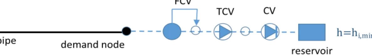
Before the full mathematical development of the approach described above, a first attempt was made by implementation of an automatic procedure that connects every demand node to a newly added series of 1 FCV (flow control valve), 1 TCV (throttle valve), 1 check valve and 1 reservoir node in an Epanet model. The FCV limits the maximum outflow to the required demand, the TCV includes the nonlinear flow-head relationship (inverse POR function) and the check valve prevents backflow from the reservoir into the system. The elevation of the reservoir is set to the elevation (minimum pressure) ℎ_’Z[ of the demand node. The setting of the FCV is the demand 𝑑 and the zeta value of the TCV is chosen such that the headloss for flow 𝑐 = 𝑑 equals the minimum service pressure ℎ_–. The modification is visualized in Figure 3.

Figure 3. Modifications in EPANET needed for PDM modelling.

The approach has been recently proposed also by other researchers. However, one important shortcoming is that the size of the model is dramatically increased by the modifications. For every demand node, an addition of three nodes and three links is required.

4.2.3 Algorithm

The algorithm can be summarized as follows:

1.) Initialization

Initialize 𝐡(,)_{, 𝐪}(,)_{, 𝐜}(,)_:

𝐡(,) _{= 𝐡}

–+ 𝟏𝒏𝒋

𝐜(,) _{= 𝐝}

and arbitrary 𝐪_,, for example 𝐪_𝒊(,)_{= 1, 𝑖 = 1, … , 𝑛𝑝.}

For nonzero demand nodes, with these starting values, all upper constraints are active and the heads are consistent. The start values for the Lagrangian multipliers are consequently λ𝒊(,)= 0, 𝑖 = 1, … , 𝑛𝑗 and

µ_𝒊(,) _{= 1, 𝑖 = 1, … , 𝑛𝑗, respectively (i.e., the upper bounds are all active and µ}

𝒊(,) is the surplus

pressure).

Initialize the following three index sets: ℐ_à(,) = ö𝑖 ∈ 𝒩|0 < 𝑐_Z(,) _{< 𝑑}

Zø = ∅ , ℐØ(,) = ö𝑖 ∈ 𝒩|𝑐Z(,) = 0ø = ∅ and ℐÙ(,) = ö𝑖 ∈ 𝒩|𝑐Z(,)=

𝑑_Zø = 𝒩

where 𝒩 is the index set of all non-zero demand junction nodes: ℐ_à(,) = ∅ , ℐ_Ø(,) = ∅ , ℐ_Ù(,)= 𝒩

2.) Iteration

Set 𝑘 = 0 Do:

Calculate the diagonal matrices 𝐄ï, 𝐍: 𝐸ï_ZZ = ùsœ

¹(˜s,™k˜s,šsT)Ï_s(ú) =

&

¹~sÏ_s(ú), 𝑁ZZ = 𝑘Z𝑐Z

(~)_{∀𝑖 ∈ ℐ}

à; 𝐸ïZZ = 0 ∀𝑖 ∈ ℐØ∪ ℐÙ and for all

zero-demand nodes.

Solve the Schur system for 𝐡(’¾&)_{− 𝐡}’_:

£𝐀I_&𝐅k&_𝐀

&+ 𝐄ï(~)¤£𝐡(~¾&)− 𝐡(~)¤ = 𝐀I&𝐅k&𝛒(Ä)É + 𝛒Ê(Ä)+ 𝐄ï(~)£𝐍(~)𝐜(~)+ 𝐡’Z[− 𝐡(~)¤

Calculate 𝐪(~¾&)_{, 𝐜} à(~¾&): 𝐪(~¾&) _{= 𝐪}(~)_{− 𝐅}k&_(𝐆£𝐪(~)_¤𝐪(~)_{− 𝐀} &𝐡(~¾&)− 𝐀,𝐡,) 𝐜_à(~¾&) _{= 𝐜} à(~)− 𝐌àk&£𝐍à(~)𝐜à(~)− 𝐡à(~¾&)+ 𝐡à,’Z[¤

Calculate multipliers:

λ_Z(~¾&) = h_Z,’Z[− ℎ_Z(~¾&) µ_Z(~¾&) _{= ℎ}

Z(~¾&)− ℎZ,¼

Check constraints and update index sets:

ℐà(~¾&) = ý𝑖 ∈ 𝒩|£𝐜Z(~¾&) > 0 ∧ 𝐜Z(~¾&) < 𝑑Z¤ ∨ h𝐜Z(~¾&) == 0 ∧ 𝜆Z(~¾&) < 0m

∨ h𝐜_Z(~¾&) _{== 𝑑}

Z ∧ 𝜇Z(~¾&) < 0m ! 4

ℐ_Ø(~¾&) _{= ý𝑖 ∈ 𝒩|h𝐜}

Z(~¾&) < 0 ∨ (𝐜Z(~¾&) == 0 ∧ 𝜆Z(’¾&) ≥ 0)m!

ℐ_Ù(~¾&) = ý𝑖 ∈ 𝒩|h𝐜_Z(~¾&) _{> 𝑑}

Z ∨ (𝐜Z(~¾&) == 𝑑Z ∧ 𝜇Z(’¾&) ≥ 0)m!

𝑐_Z(~¾&) = max£𝐜_Z(~¾&)_{, 0¤ ∀𝑖 ∈ ℐ} à(~)

𝑐_Z(~¾&) = min£𝐜_Z(~¾&)_{, 𝑑}

Z¤ ∀𝑖 ∈ ℐà(~)

while convergence not reached.

4.2.4 Matlab implementation at 3S Consult

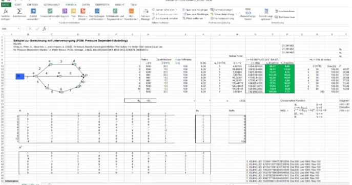
The method previously presented was implemented using Matlab and applied to a small network. For this small system, the iterative calculation was also implemented in Excel (Path-GGA-Iterations_v10.xlsx is additionally provided). It was also the basis of the description of the iterative method (see Figure 4).

Basically, all the steps which were described by Excel operations were then translated into Matlab. This implementation was supported by an Epanet-Matlab Toolkit, which allows the user to open the INP network files in Matlab, and read the network properties (pipe lengths, pipe diameters, roughness, nodes demands, node elevations, etc.).

The major challenge was to create the incidence matrix of the network, which was the only element to be done from scratch. Following the steps already checked in Excel, the algorithm has converged after 8-9 iterations for this network.

4 _{The statement A ∨ B is true if A or B (or both) are true; The statement A ∧ B is true if A and}

Figure 4. Excel implementation for a simple network.

For the sake of simplicity, the chosen headloss formula was Hazen-Williams; nonetheless, also the Darcy-Weisbach head loss formula was correctly developed.

The iterative method was further tested for a range of networks with increasing complexity in terms of number of nodes and pipes. In Table 1, the main characteristics for each network are shown. Since we focused on steady-state calculations, there is no difference between reservoirs and tanks (the latter have a time-dependent water level). Moreover, not all nodes are demand ones. All the networks have a Darcy-Weisbach headloss equation and LPS as flow unit.

For the stopping criterion, two relative thresholds were chosen, named “epsilonq” and “epsilonh”, which refer respectively to pipe flow limit and node head limit (here it was relatively restricting 10-10_{, but the}

quadratic convergence was observed). Also, a maximum number of iterations of 30 was taken. The service minimum pressure is equal to 30 m (3 bar) and the minimum pressure is the elevation:

ℎ_Z,’Z[ = 𝑧_Z 𝑎𝑛𝑑 ℎ_Z,– = 𝑧_Z+ 30.

Table 1. The test networks and their properties.

Name n° nodes n° pipes n° dem. nodes n° res./tanks

n1Dim932x848 848 932 474 (55.9%) 2R+6T n2Dim1118x1039 1039 1118 661 (63.6%) 2R n3Dim1975x1770 1770 1975 1770 (100%) 4R n4Dim2465x1890 1890 2465 1609 (85.1%) 3R n5Dim2509x2443 2443 2509 1241 (50.8%) 2T n6Dim8585x8392 8392 8585 3173 (37.8%) 2T n7Dim14830x12523 12523 14830 10552(84.2%) 7R

n8Dim19647x17971 17971 19647 15332 (85.3%) 15R

For the four following tests, various indicators were reported: the number of iterations needed by the solver to reach convergence; how many (demand) nodes are fully supplied (IU); the number of nodes in

reduced-supply condition (IA); the number of nodes in failure mode (IL; and finally, the percentage of

demand satisfaction Dred for the full system. The first set of tests was done with default data, with

demand multiplier equal to 1 (Table 2):

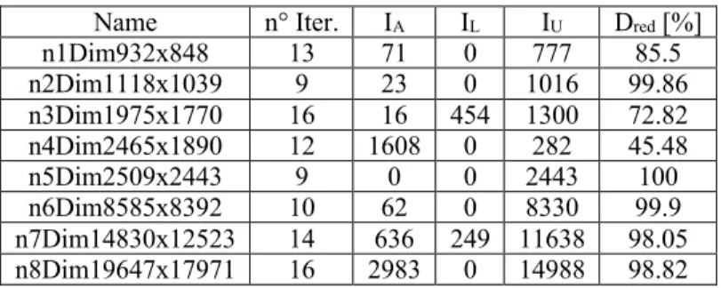
Table 2. PDM parameter for each test Network.

Name n° Iter. IA IL IU Dred [%]

n1Dim932x848 13 71 0 777 85.5 n2Dim1118x1039 9 23 0 1016 99.86 n3Dim1975x1770 16 16 454 1300 72.82 n4Dim2465x1890 12 1608 0 282 45.48 n5Dim2509x2443 9 0 0 2443 100 n6Dim8585x8392 10 62 0 8330 99.9 n7Dim14830x12523 14 636 249 11638 98.05 n8Dim19647x17971 16 2983 0 14988 98.82

At a first glance, one can say that an increase of the number of demand nodes, combined with the number of reservoir/tanks, can affect the number of iterations needed to find a solution (the network is more complex). In most cases, the nodes are either fully supplied or in PDM mode.

Then the demand multiplier was increased step-wise to 1.5 and 2 for a progressive increase in demand and then 5 to explore the effects of heavy PDM conditions (Tables 3 to 5):

Table 3. Solver results with demand mult. = 1.5.

Name n° Iter. IA IL IU Dred [%]

n1Dim932x848 13 74 0 774 85.25 n2Dim1118x1039 8 40 0 999 99.74 n3Dim1975x1770 16 8 533 1229 68.35 n4Dim2465x1890 13 1566 42 282 34.15 n5Dim2509x2443 10 0 0 2443 100 n6Dim8585x8392 10 94 0 8298 99.56 n7Dim14830x12523 15 2637 262 9624 94.32 n8Dim19647x17971 14 3699 0 14272 98.36

Table 4. Solver results with demand mult. = 2.

Name n° Iter. IA IL IU Dred [%]

n1Dim932x848 13 92 0 756 84.8 n2Dim1118x1039 8 57 0 982 99.46 n3Dim1975x1770 16 9 589 1172 64.92 n4Dim2465x1890 13 1548 60 282 27.1 n5Dim2509x2443 10 0 0 2443 100 n6Dim8585x8392 11 126 0 8266 98.09 n7Dim14830x12523 16 5269 339 6915 88.13

n8Dim19647x17971 14 4247 0 13724 97.8

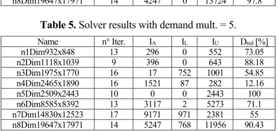
Table 5. Solver results with demand mult. = 5.

Name n° Iter. IA IL IU Dred [%]

n1Dim932x848 13 296 0 552 73.05 n2Dim1118x1039 9 396 0 643 88.18 n3Dim1975x1770 16 17 752 1001 54.85 n4Dim2465x1890 16 1521 87 282 12.16 n5Dim2509x2443 10 0 0 2443 100 n6Dim8585x8392 13 3117 2 5273 71.1 n7Dim14830x12523 17 9171 971 2381 55 n8Dim19647x17971 14 5247 768 11956 90.43

The results show that for each network, a fast convergence is reached, independently of the value of the demand multiplier. From the indicator results as expected, the higher the demand multiplier is, the more nodes find themselves in under-supply or even no-supply/failure mode state.

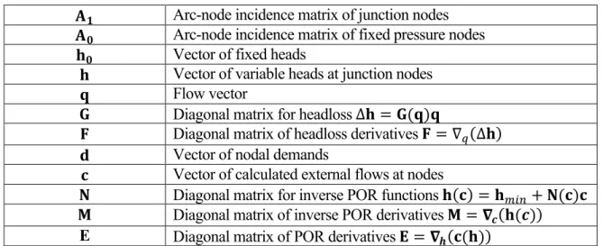
5 NOMENCLATURE

Table 6. Matrices and vector notations.

𝐀_𝟏 Arc-node incidence matrix of junction nodes 𝐀_𝟎 Arc-node incidence matrix of fixed pressure nodes 𝐡_𝟎 Vector of fixed heads

𝐡 Vector of variable heads at junction nodes 𝐪 Flow vector

𝐆 Diagonal matrix for headloss Δ𝐡 = 𝐆(𝐪)𝐪

𝐅 Diagonal matrix of headloss derivatives 𝐅 = ∇_d(Δ𝐡) 𝐝 Vector of nodal demands

𝐜 Vector of calculated external flows at nodes

𝐍 Diagonal matrix for inverse POR functions 𝐡(𝐜) = 𝐡_’Z[+ 𝐍(𝐜)𝐜 𝐌 Diagonal matrix of inverse POR derivatives 𝐌 = 𝛁_𝒄(𝐡(𝒄))

6 CONCLUSION

A suitable optimisation framework was developed for dealing with large disconnected subnetworks undergoing a partially or full system collapse. Two solution methods were derived from the pressure-driven PDM Content minimisation problem formulation.

The first one is a primal-dual Newton method applied on the reduced Lagrangian of the problem that was published in the Journal of Water Resources Planning and Management (Elhay et al, 2016). It requiries solving a linear system at each iteration for the nodal heads, then the pipe flow rates are updated. Due to the sub-linearity of the pressure outflow relationship (the Wagner POR is a square root function) in some situation an under-relaxation of the iterates is necessary. It is done using the damped Newton method with an inexact line search of Goldstein type. This means that additional evaluation of the criterion to optimize is needed. As a matter of acceleration, an equivalent Least-squares formulation involving the mass and energy residuals was derived. It is implemented in Matlab and will be part of the Irstea software solution, Porteau.

The second one is a primal projected Newton method applied to the PDM Content problem. It is fully described in this report. It is considering the nodal consumption that is bounded between zero and the demand and two additional dual variables, the pressure surplus above the service head and the deficit pressure below the minimum head (in fact the node elevation). These two last variables are nonnegative and interpreted as KKT or Lagrange multipliers. The linear system for solving for the nodal head possesses an additional term in the second member but the iteration matrix is the same. The update for the flow is the same. There are three additional equations for calculating the nodal consumptions at demand nodes and the two Lagrange multipliers. Three index sets help managing the active/inactive primal constraints and the KKT conditions. It was validated on a small network and eight large networks (the same than for the first method). For all the tests made, it is converging without the need of a stepsize correction. One explanation is that both the pipe head losses and the nodal inverse POR functions are convex monotonic functions of the pipe flow rates and the nodal consumptions.

In the next six months, it is planned to apply the two robust solutions for case studies from the ResiWater project provided by BWB and EMS in Germany and France. It is necessary to consider control valves and pumps and the solution will be detailed in the deliverable report D4.2.

7 REFERENCES

Bhave, P. R. (1981). "Node Flow Analysis Distribution Systems." Transportation Engineering Journal, 107(4), 457-467.

Birkhoff, G.: A variational principle for nonlinear networks, Quart. Appl. Math, 21, 160–162, 1963.

Braun M., Piller O., Deuerlein J. and Mortazavi I. (2016). "Limitations of Demand- and Pressure-Driven Modeling for Large Deficient Networks." CCWI 2016 conference, Amsterdam, 8 pages. Carpentier P., Cohen G., and Hamam Y. (1985). “Water network equilibrium, variational formulation and comparison of numerical algorithms”, EURO VII, 1985.

Collins, M., Cooper, L., Helgason, R., Kennington, R., and Leblanc, L. (1978). "Solving the Pipe Network Analysis Problem using Optimization Techniques." Management Science, 24(7), 747-760.

Cross, H. (1936). "Analysis of Flow in Networks of Conduits or Conductors." Bulletin No. 286, University of Illinois Engineering Experimental Station.)

Deuerlein, J. W. (2008). "Decomposition Model of a General Water Supply Network Graph." Journal of Hydraulic Engineering, 134(6), 822-832.

Deuerlein, J., Simpson, A., and Montalvo, I. (2012). "Preprocessing of Water Distribution Systems to Assess Connectivity and Solvability in the Presence of Flow Control Devices." World Environmental and Water Resources Congress 2012, E. D. Loucks, ed., Albuquerque, New Mexico, United States, 3237-3247.

Elhay, S., Piller, O., Deuerlein J. and Simpson, A. R., M. ASCE. “A robust, rapidly convergent method that solves the water distribution equations for pressure-dependent models” J. Water Resour. Plann. Manage., 142(2), 2016.

Gorev, N. B., Kodzhespirova, I. F., and Sivakumar, P. (2016). "Nonunique Steady States in Water Distribution Networks with Flow Control Valves." Journal of Hydraulic Engineering, 142(9), 04016029-1:04016029-7.

Piller, O. (1995). "Modeling the behavior of a network - Hydraulic analysis and sampling procedures for parameter estimation," Applied Mathematics thesis from the University of Bordeaux (PRES), defended on, 288 pages, Talence, France.

Piller, O., and Van Zyl, J. E. (2007). "A unified framework for pressure driven network analysis." Water Management Challenges in Global Change (CCWI2007 and SUWM2007 Conference), Leicester, UK, Volume 2/2, 25-30.

Piller, O., and van Zyl, J. E. (2009). "Pressure-Driven Analysis of Network Sections Supplied Via high-lying Nodes." Computing and Control in the Water Industry 2009 'Integrating Water Systems', The Edge, University of Sheffield, printed by CRC press/Balkema, Volume 1/1, 257-262.

Piller, O., Brémond, B., and Poulton, M. (2003). "Least Action Principles Appropriate to Pressure Driven Models of Pipe Networks." World Water and Environmental Resources Congress (EWRI03), Philadelphia (PA), US, printed by ASCE, (CD-ROM).

SMaRT-OnlineWDN _{(2017), http://www.smart-onlinewdn.eu/, last accessed on 17}th _{February 2017.}

van Zyl, J., and Cassa, A. (2014). "Modeling Elastically Deforming Leaks in Water Distribution Pipes." Journal of Hydraulic Engineering, 140(2), 182-189.

Wagner, J. M., Shamir, U., and Marks, D. H. (1988). "Water Distribution Reliability: Simulations Methods." Journal of Water Resources Planning and Management, 114(3), 276-294.