HAL Id: hal-00516518
https://hal.archives-ouvertes.fr/hal-00516518
Submitted on 24 Dec 2015
HAL is a multi-disciplinary open access
archive for the deposit and dissemination of
sci-entific research documents, whether they are
pub-lished or not. The documents may come from
teaching and research institutions in France or
abroad, or from public or private research centers.
L’archive ouverte pluridisciplinaire HAL, est
destinée au dépôt et à la diffusion de documents
scientifiques de niveau recherche, publiés ou non,
émanant des établissements d’enseignement et de
recherche français ou étrangers, des laboratoires
publics ou privés.
retrieved for the first time from the IASI/MetOp
thermal infrared sounder
A. Razavi, F. Karagulian, Lieven Clarisse, Daniel Hurtmans, Pierre-François
Coheur, Cathy Clerbaux, Jean-François Müller, T. Stavrakou
To cite this version:
A. Razavi, F. Karagulian, Lieven Clarisse, Daniel Hurtmans, Pierre-François Coheur, et al.. Global
distributions of methanol and formic acid retrieved for the first time from the IASI/MetOp thermal
infrared sounder. Atmospheric Chemistry and Physics, European Geosciences Union, 2011, 11 (2),
pp.857-872. �10.5194/acp-11-857-2011�. �hal-00516518�
www.atmos-chem-phys.net/11/857/2011/ doi:10.5194/acp-11-857-2011
© Author(s) 2011. CC Attribution 3.0 License.
Chemistry
and Physics
Global distributions of methanol and formic acid retrieved for the
first time from the IASI/MetOp thermal infrared sounder
A. Razavi1, F. Karagulian1,*, L. Clarisse1,**, D. Hurtmans1, P. F. Coheur1,**, C. Clerbaux2,1, J. F. M ¨uller3, and T. Stavrakou3
1Service de Chimie Quantique et Photophysique, Universit´e Libre de Bruxelles (U.L.B.), Brussels, Belgium 2UPMC Univ. Paris 06; Universit´e Versailles St-Quentin; CNRS/INSU, LATMOS-IPSL, Paris, France 3Belgian Institute for Space Aeronomy (BIRA-IASB), Brussels, Belgium
*now at: European Commission, Joint Research Centre (JRC), 21027 Ispra, Italy
**These authors are respectively Postdoctoral Researcher and Research Associate with FRS-FNRS, Belgium
Received: 15 July 2010 – Published in Atmos. Chem. Phys. Discuss.: 8 September 2010 Revised: 14 January 2011 – Accepted: 24 January 2011 – Published: 31 January 2011
Abstract. Methanol (CH3OH) and formic acid (HCOOH)
are among the most abundant volatile organic compounds present in the atmosphere. In this work, we derive the global distributions of these two organic species using for the first time the Infrared Atmospheric Sounding Interferometer (IASI) launched onboard the MetOp-A satellite in 2006. This paper describes the method used and provides a first criti-cal analysis of the retrieved products. The retrieval process follows a two-step approach in which global distributions are first obtained on the basis of a simple radiance indexing (transformed into brightness temperatures), and then mapped onto column abundances using suitable conversion factors. For methanol, the factors were calculated using a complete retrieval approach in selected regions. In the case of formic acid, a different approach, which uses a set of forward sim-ulations for representative atmospheres, has been used. In both cases, the main error sources are carefully determined: the average relative error on the column for both species is estimated to be about 50%, increasing to about 100% for the least favorable conditions. The distributions for the year 2009 are discussed in terms of seasonality and source iden-tification. Time series comparing methanol, formic acid and carbon monoxide in different regions are also presented.
Correspondence to: A. Razavi
1 Introduction
Volatile Organic Compounds (VOCs) includes thousands of different carbon-containing gases present in our atmosphere at concentrations ranging from less than a pptv to more than a ppmv (only methane exceeds 1 ppmv and is usually excluded from the VOC definition). Emitted from a large variety of processes (biogenic or anthropogenic) at the Earth’s surface, they have an important influence on the atmospheric com-position and climate. VOCs are precursors to tropospheric ozone (Houweling et al., 1998), they play an important role on the oxidizing capacity of the troposphere (Atkinson and Arey, 2003; Monks, 2005), they lead to the formation of sec-ondary organic aerosols (Tsigaridis and Kanakidou, 2007; Heald et al., 2008) and they impact on climate change in different indirect ways (Meinshausen et al., 2006; Feingold et al., 2003; Charlson et al., 1987). In order to better under-stand and quantify their emissions and the role they play in the Earth’s system, it is important to assess their atmospheric distribution at the global scale.
1.1 Observation of VOCs from space
The first steps in measuring volatile organic compounds by infrared satellite sounders were made during the last years, mostly using high-sensitive limb-viewing instruments. Methanol and formic acid, along with a series of other com-pounds, have been observed in young or aged biomass burn-ing plumes with the ACE-FTS instrument (Rinsland et al., 2004; Dufour et al., 2006; Coheur et al., 2007; Rinsland et al., 2007; Herbin et al., 2009). Large datasets of that sounder, covering several years, have been gathered to provide quasi-global distributions of these two species and to study their seasonal variability (Rinsland et al., 2006; Dufour et al.,
2007; Abad et al., 2009). Similarly the observations of the MIPAS limb emission sounder have enabled mapping upper tropospheric distributions of several organic species such as PAN (Glatthor et al., 2007; Moore and Remedios, 2010), ace-tone (Moore et al., 2010) as well as HCN and C2H6(Glatthor
et al., 2009); very recently global distributions of formic acid have also been gathered and analyzed (Grutter et al., 2010). The possibility of probing these VOCs lower in the atmo-sphere using nadir infrared sounders was suggested based on local observations, both by TES (Beer et al., 2008) and IASI (Coheur et al., 2009), in the latter case in large biomass burning plumes.
Other VOC observations from space have been performed using ultraviolet (UV) sounders. The GOME and OMI in-struments provide measurements of formaldehyde (Chance et al., 2000; Millet et al., 2008b), providing constraints on the emissions of isoprene (Shim et al., 2005; Palmer et al., 2006) and other non-methane volatile organic com-pounds (NMVOCs) (Fu et al., 2007; Stavrakou et al., 2009). With the complementary use of SCIAMACHY (De Smedt et al., 2008) and with the GOME follow-on instrument on-board MetOp-A (GOME-2), a long-term dataset (14 years) of formaldehyde observations is now available. In addi-tion, measurements of glyoxal have also been made from the SCIAMACHY instrument (Wittrock et al., 2006; Vrekoussis et al., 2009).
This study provides the first global distributions of methanol and formic acid observed by the IASI (Infrared Atmospheric Sounding Interferometer) instrument (Phulpin et al., 2007), briefly described in Sect. 2.1. This infrared nadir-looking sounder has already demonstrated its poten-tial for the monitoring of different trace gases such as CO (George et al., 2009; Turquety et al., 2009), O3 (Boynard
et al., 2009), CH4(Razavi et al., 2009) and HNO3(Wespes
et al., 2009). IASI has also demonstrated its high sensitivity to weak absorbers such as NH3, for which global and local
distributions have been obtained (Clarisse et al., 2009, 2010). The same method as the one used for retrieving global NH3,
and which relies on a simple difference of brightness temper-atures, has been adapted to retrieve methanol and formic acid total columns. The method is described in Sect. 2.2 and a critical analysis of the resulting methanol field is provided in Sect. 3. The latter includes a first interpretation of the global distributions and seasonality of methanol as well as an error analysis. Section 4 provides similar analysis for formic acid. In addition, time series comparing the two species and CO for selected regions are presented in Sect. 5.
Prior to this, a review of sources, sinks and previous mea-surements of methanol and formic acid is provided.
1.2 Methanol
Methanol (CH3OH) is the most abundant organic species in
the Earth’s atmosphere after methane and is also the main non-methane organic volatile compound in the mid to
up-per troposphere (Heikes et al., 2002). Because its main re-moval process is oxidation by OH (Atkinson, 1986), CH3OH
has a noticeable impact on the oxidizing capacity of the tro-posphere and on the global budget of tropospheric ozone (Tie et al., 2003). Additional sinks include removal by dry and wet deposition and uptake by the ocean (Jacob et al., 2005; Millet et al., 2008a). Its mean lifetime is evaluated to be about 10 days in the free troposphere. The main emis-sion sources of methanol are biogenic processes, involving plant growth (MacDonald and Fall, 1993; Nemecek-Marshall et al., 1995; Harley et al., 2007; Galbally and Kirstine, 2002) and plant decay to a lesser extent (Warneke et al., 1999). Other sources include biomass burning (Holzinger et al., 2005), oxidation of methane and other VOCs, as well as an-thropogenic emissions from vehicles and industrial activities (Singh et al., 2000). There still exists large uncertainties in the relative source strengths, the atmospheric distribution and budget of CH3OH (Singh et al., 2000; Tie et al., 2003; Jacob
et al., 2005).
During the past few years, coordinated measurement cam-paigns have been conducted which provide, among other trace species, in situ and aircraft determination of methanol abundances, and from there information about its different emission sources. The diurnal and seasonal cycle of CH3OH
has been studied from in situ measurement in different types of environments such as forest (Karl et al., 2003, 2005), ru-ral (Schade and Goldstein, 2006; Brunner et al., 2007; Jor-dan et al., 2009) or urban areas (Filella and Pen¸uelas, 2006; Nguyen et al., 2001) with a variety of techniques. The con-centrations usually increase during daytime due to the light induced release of methanol by plants. Moreover, CH3OH
abundances are found to be higher during spring because of high plant growth emissions during that season. Methanol concentrations of about 4 ppbv have been reported in the amazonian region (Karl et al., 2007; Eerdekens et al., 2009). Aircraft measurements were also carried out over oceans (Singh et al., 2000, 2004) where background concentrations of a few hundreds of pptv were found. Airborne observations led also to the study of CH3OH in several biomass burning
plumes (Yokelson et al., 1999; Fischer et al., 2003; Yokelson et al., 2003; Holzinger et al., 2005) where volume mixing ratios (vmr) of up to several tens of ppbv were found. Ob-servations of CH3OH with ground-based infrared
spectrom-eters were also recently conducted in Australia (Paton-Walsh et al., 2008) and in Arizona (Rinsland et al., 2009). The latter study provides an unprecedented 22 years time series of free tropospheric CH3OH; it does not report any significant trend
over the years but shows a clear seasonality with a maximum in early July and a minimum during January.
The quasi-global distributions obtained from ACE-FTS (Dufour et al., 2007) have further revealed that the surface sources of methanol have a significant impact on its up-per tropospheric concentrations, which are mostly driven by biogenic and biomass burning emissions in the Northern and Southern Hemisphere, respectively. Beer et al. (2008)
has firstly demonstrated the possibility to measure methanol from a nadir infrared sounder and reports lower CH3OH
con-centrations in California than near Beijing, where emissions could be caused by local sources.
The strongest absorption band of methanol in the infrared is the ν8 CO-stretching mode centered at 1033cm−1. We
have used line parameters of Xu et al. (2004), implemented in the HITRAN database for which a precision of 6% for line intensities is quoted.
1.3 Formic acid
Formic acid (HCOOH) is one of the most abundant organic acid and has a strong influence on pH-dependent chemical reactions in clouds (Keene and Galloway, 1988). It has also been identified as a major sink for OH reactions in cloud wa-ter (Jacob, 1986). Although its sources and sinks are still poorly quantified, HCOOH is known to be emitted by var-ious processes: biomass burning (Goode et al., 2000; Wor-den et al., 1997; Yokelson et al., 1997), biogenic emissions from vegetation (Keene and Galloway, 1984, 1988), emis-sions from soil (Sanhueza and Andreae, 1991), from ants (Graedel and Eisner, 1988), as a secondary product from organic precursors (Rasmussen and Khalil, 1988; Arlander et al., 1990) and also from motor vehicles (Kawamura et al., 1985; Grosjean, 1989). Formic acid can be also produced from the aqueous oxidation of formaldehyde in cloud and rain water (Chameides and Davis, 1983) as well as from the oxidation of formaldehyde by HO2 radicals in the cold
tropopause region (Hermans et al., 2005). It is mainly re-moved from the troposphere through wet and dry deposition but also through oxidation by the OH radical to a lesser ex-tent. The resulting lifetime of HCOOH, estimated to be a few days in the boundary layer, increases in the free tro-posphere because of the scarcity of precipitation (Sanhueza et al., 1996). HCOOH has been found to be a product of the isoprene oxidation by ozone (Jacob and Wofsy, 1988; Mar-tin et al., 1991) and by OH radicals, in particular through the OH-oxidation of glycolaldehyde (Butkovskaya et al., 2006a) and hydroxyacetone (Butkovskaya et al., 2006b), which are two important isoprene oxidation products, but also through the OH-oxidation of isoprene nitrates (Paulot et al., 2009).
In situ measurements of formic acid in the boundary layer have been carried out using different techniques in various parts of the world, from rural sites (Talbot et al., 1988; Puxbaum et al., 1988; Talbot et al., 1990; Hartmann et al., 1991; Helas et al., 1992) to urban areas (Grosjean, 1989; Khwaja, 1995; Granby et al., 1997; Souza et al., 1999). The observed HCOOH volume mixing ratio in the boundary layer ranges from 0.01 to 10 ppbv. Its diurnal cycle shows larger concentrations in the mid- to late afternoon (Martin et al., 1991; Hartmann et al., 1991) indicating larger sources during daytime (biogenic emission, photochemical reactions) and dry deposition at nighttime.
HCOOH measurements in the upper troposphere, per-formed during several aircraft campaigns (Reiner et al., 1999; Jaegl´e et al., 2000; Singh et al., 2000), have re-ported mixing ratios from about 30 to 215 pptv. HCOOH has also been probed in different biomass burning plumes (Yokelson et al., 1999; Goode et al., 2000; Herndon et al., 2007) with concentrations of around ten ppbv; Worden et al. (1997) reported HCOOH total columns of 8.6 and 11.2 × 10¹⁶molec cm−2above two fire events in the USA using op-tical measurements in the infrared. Similar spectral measure-ments, which used the HCOOH ν6 absorption band in the
IR, were performed from a balloon (Goldman et al., 1984; Remedios et al., 2007), with mixing ratios up to 600 pptv at about 7 km height, or from the ground (Rinsland et al., 2004). The latter study gives insight on the seasonal vari-ation of HCOOH, with a mean mixing ratio in the free tro-posphere from about 300 pptv in October–December to about 800 pptv in July–September, likely resulting from higher bio-genic emissions during the growing season. Other ground-based measurements above Jungfraujoch were very recently analyzed over a 22 years period and show a similar seasonal cycle with a maximum occurring during summer as well as significant diurnal and day-to-day variability (Zander et al., 2010).
The first satellite observations in the upper troposphere were reported from the ACE-FTS instrument (Rinsland et al., 2006, 2007; Coheur et al., 2007) and were correlated to biomass burning events. Recent work performed with ACE-FTS on quasi-global observations of HCOOH reported an av-erage mixing ratio of about 0.3 ppbv in the free troposphere with hot spots of up to 0.59 ppbv in tropical regions (Abad et al., 2009). Very recent global distributions were also as-sessed by the MIPAS sounder (Grutter et al., 2010) over a 6 years period. They report seasonal variations that may be associated to biogenic emissions with higher mixing ra-tios at 8 km during summer (about 100 pptv) than in winter (about 45 pptv). High concentrations were also observed in biomass burning plumes in the Southern Hemisphere. The nadir-viewing IASI sounder has also recently demonstrated the possibility to observe the HCOOH spectral signature in fire plumes (Coheur et al., 2009). In this study, we pro-vide the first distributions of formic acid total columns above land, differentiated into four seasons for the year 2009. The retrieval method is slightly different from the one used for methanol because the conversion factor between brightness temperature differences and total columns is derived from a set of forward simulation. Details and error estimation are provided in Sect. 4.1.
We have used a new set of HCOOH spectroscopic line pa-rameters of Vander Auwera et al. (2007), implemented in the latest versions of HITRAN and GEISA databases. The accuracy on the absolute line intensities is evaluated to be about 7%. The updated data set reports HCOOH line inten-sities larger by about a factor 2 compared to previous stud-ies (Perrin and Vander Auwera, 2007). This implstud-ies that
concentrations obtained from infrared retrievals before 2007 were likely too high by the same factor.
2 Instrument and method 2.1 Description of IASI
The IASI instrument, launched onboard the MetOp-A plat-form in October 2006 in a polar sun-synchronous orbit, is a nadir-looking Fourier transform spectrometer that records the Earth’s outgoing radiation from 645 to 2760 cm−1
with-out gaps at an apodized resolution of 0.5 cm−1. Its field of view is a 2×2 matrix of circular pixels which have a 12 km footprint diameter at nadir. IASI provides two global Earth coverages per day (about 1 280 000 spectra) thanks to the wide scans across its track (2200 km swaths). It offers also a very good signal-to-noise ratio, with a Noise Equiv-alent Delta Temperature (NEDT) at 280 K of about 0.2 K in the spectral region of interest (which extends from 975 to 1150 cm−1). Moreover, with the successive launch of two other identical instruments, the IASI mission will provide consistent measurements over a 15 years period. A technical description of IASI and examples of applications for chem-istry can be found in the review of Clerbaux et al. (2009). The IASI calibrated radiance spectra are disseminated in near-real time by the EumetCast system along with temperature, humidity profiles and cloud information (coverage, temper-ature and altitude). Only cloud free observations (when the cloud coverage for the pixel is below 2%) are taken into ac-count for this study.
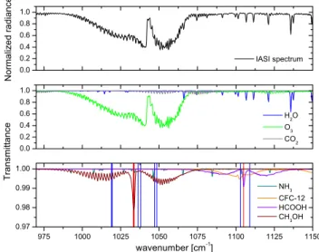
The measurement of methanol and formic acid concen-trations from IASI is quite challenging due to their weak absorption and the interference of other molecules in the same spectral range (see Fig. 1). CH3OH is observable
using its C−O stretching absorption band located around 1033 cm−1. The spectral range also covers the ν6absorption
band of HCOOH located near 1105 cm−1 and the ν3 band
of trans−HCOOH at 1777 cm−1(Perrin et al., 2009), which cannot be detected in the IASI spectra because of strong wa-ter vapor inwa-terferences.
2.2 Retrieval approach
In order to take advantage of the very good spatial coverage of IASI we have chosen a simple, fast and robust approach based on brightness temperature differences (1Tb), similar
to the method already used for the retrieval of sulfur dioxide (Clarisse et al., 2008) and ammonia (Clarisse et al., 2009). It consists in two steps: (i) the determination of 1Tbglobally
and (ii) the conversion of 1Tbto total column amounts
us-ing one (global) or two (continental and oceanic) conversion factors.
The 1Tbcorresponds to the difference between the
bright-ness temperatures measured in one or several channels se-lected in the absorption signature of the target molecule
Fig. 1. Top panel: IASI normalized radiance spectrum in the
spec-tral region between 950 and 1200 cm−1 containing methanol and formic acid absorption bands. Bottom panels: Contribution to the IASI spectrum of different atmospheric species plotted in transmit-tance. The vertical lines indicate the target channels (in red) and the baseline channels (in blue) which are used for the 1Tb
determina-tion (nine channels are used for CH3OH, and three for HCOOH). See Sect. 2.2 for details.
(Tb,target) and the brightness temperature of nearby channels
selected in a spectral region where the least absorptions are found (Tb,0). This is expressed in the following equation as
1Tb= hTb,0i − hTb,targeti (1)
This quantity gives a handy estimate for the strength of absorption and hence of the concentration. However, the physics of the radiative transfer is not accounted for and the conversion of 1Tb to total columns requires a full
radia-tive transfer treatment. For this purpose, we have retrieved CH3OH total columns at various locations of the world with
an inversion model based on the Optimal Estimation Method (OEM) (Rodgers, 2000) that includes a line-by-line radia-tive transfer model. This is implemented in the Atmosphit software developed at the Universit´e Libre de Bruxelles (for more information see Clarisse et al., 2008 and Coheur et al., 2005). The method is only applied in selected regions due to computational limitations. The conversion factor derived by matching the retrieved columns on the corresponding 1Tbis
applied globally to derive the total column distributions. For HCOOH, we used an alternative conversion method only based on forward simulations (see Sect. 4.1).
In the next two sections we describe the different retrieval parameters (the chosen channels, spectral intervals and a pri-ori information) and present the resulting global distributions for CH3OH and HCOOH, respectively.
3 Methanol retrieval and distributions 3.1 Retrieval settings
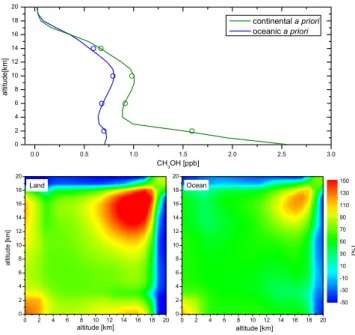
Methanol a priori profiles and covariance matrices were de-rived from distributions calculated by the IMAGESv2 global chemistry-transport model (Stavrakou et al., 2009). Monthly averaged model profiles over the whole year 2007 were used globally, on a 4◦×5◦latitude-longitude grid to account for the seasonal and spatial variability of the model. Two dif-ferent vertical profiles were selected: an average continental and an average oceanic profile. This choice is justified by the existence of strong emission over continents resulting in enhanced concentrations in the boundary layer. These two profiles are illustrated on Fig. 2 together with their associ-ated covariance matrix (where the diagonal elements repre-sent the model variability for the profile, and the off-diagonal elements represent the correlation between values at different altitudes). The continental a priori profile has a surface mix-ing ratio of about 2.5 ppbv, about four times larger than in the oceanic profile. Above 4 km, the two profiles are similar with only slightly higher concentrations for the continental profile. The covariance matrices both show higher variabili-ties in the lower (0 to 2 km) and upper (14 to 18 km) tropo-sphere. Over continental surfaces, the variabilities are larger by about 25%. In both cases, the correlation length is large.
As can be seen from Fig. 1, the methanol spectral signa-ture is fully overlapped by the much stronger ozone band at 10 µm. A large spectral range is therefore needed in or-der to properly account for this strong interference in the re-trieval process. The spectral range extending from 981.25 to 1038 cm−1was selected after several tests. CH
3OH
par-tial columns are retrieved in 4 km thick layers from the ground to 16 km. Partial columns of O3 in 6 layers up to
42 km and the total columns of H2O and NH3 are
simul-taneously adjusted. The regions selected for the retrievals are described in Table 1. These regions/periods were se-lected because of their high 1Tb values and no significant
seasonal differences have been noticed. An example of in-version is presented on Fig. 3 (top panel) for a case where the CH3OH signature is unambiguous. The RMS of the
residue when CH3OH is not included in the retrieval is
sig-nificantly higher (3.1 × 10⁻⁶W/(m2sr m−1)) than when it is taken into account (2.5×10⁻⁶W/(m2sr m−1)), this value be-ing very close to the theoretical noise. This specific retrieval leads to a methanol total column of 5.57 × 10¹⁶molec cm−2.
Retrieved methanol mixing ratios in the lowermost atmo-spheric layer (0 to 4 km) range from about 0.1 to 7.0 ppb for the different selected regions. Comparisons between model data optimized with the IASI methanol product and previous CH3OH measurements (in situ and aircraft) were carried out
and are detailed in the latest work by Stavrakou et al. (sub-mitted to ACP). On the bottom panel of Fig. 3, representative total column averaging kernels differentiated for continen-tal and oceanic retrievals are illustrated. They correspond to
Fig. 2. Top panel: Illustration of the two CH3OH a priori profiles
(continental and oceanic) derived from the IMAGESv2 CTM model for the year 2007. Open circles represent the a priori on the 4 layers retrieval grid. Bottom panels: Plot (expressed in %) of the associ-ated covariance matrices (left: for land, right: for ocean).
Table 1. Selected regions and periods for the retrieval of methanol
using the Optimal Estimation Method.
Localization Region Date DOFS range Congo 0 − 35◦S 20 October 2008 0.29–1.02 10 − 50◦E Chad 0 − 25◦N 5 April2009 0.77–1.05 0 − 30◦E Brazil 0 − 20◦S 20 October 2008 0.45–1.02 35 − 60◦W India 5 − 40◦S 2 May 2009 0.50–1.06 70 − 90◦E Atlantic 30◦S – 25◦N 11 August 2008 0.12–0.87 10 − 40◦W
the mean averaging kernels for all retrievals performed in the selected regions. In both cases, the sensitivity is maximum in the mid to upper troposphere from about 5 to 11 km, but retrievals over land show much higher sensitivity near the ground, largely due to the higher thermal contrast (Clerbaux et al., 2009). The resulting DOFS (Degrees Of Freedom for Signal, given by the trace of the averaging kernel matrix) for these retrievals are given in Table 1. DOFS values range from 0.29 to 1.06 over land and are found lower above the ocean (between 0.12 and 0.87) where the dependence on the a priori is therefore larger.
Fig. 3. Top panel: Example of a methanol retrieval from an IASI
spectrum recorded over Namibia (20.16◦S–21.50◦E) on 20 Octo-ber 2008. The observed (blue curve) spectrum is shown together with the fit residue (in cyan) and the dashed horizontal lines de-limit this residue by its RMS value. The dark green curve is the fit residue when CH3OH is not taken into account in the retrieval, the
red curve represents the calculated CH3OH contribution to the
spec-trum and the dashed vertical line indicates the detectable CH3OH
absorption band. Bottom panel: Mean total column averaging ker-nels presented for retrievals performed over land (green curve) and over ocean (blue curve).
For the global 1Tbcalculation, the three target channels,
all chosen in the Q-branch of CH3OH (at 1033.25, 1033.5
and 1033.75 cm−1, see Fig. 1), are also contaminated by O3.
Therefore, the baseline channels were also chosen inside the O3absorption band (at 1019, 1019.5, 1036.25, 1038, 1047
and 1048.5 cm−1, see Fig. 1) in a way that maximizes the sensitivity of 1Tb to the CH3OH amount. To deal with
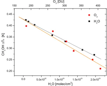
the remaining contribution of O3, the relationship between
1Tband O3 concentrations has been derived using a set of
forward simulations. For different columns of O3 (ranging
from 185 to 407 DU), the spectrum and 1Tbwere calculated
with a fixed amount of CH3OH (4 × 10¹⁶molec cm−2). The
results, presented on Fig. 4 assuming a typical midlatitude summer atmosphere (1976 US standard model), show an ap-proximately linear correlation between the total column of ozone and the calculated 1Tb. Similar results were obtained
for other typical atmospheres and an average linear depen-dence was computed (with a slope of 9.02 × 10⁻⁴K DU−1).
Fig. 4. Illustration of the influence of water vapor and ozone
con-centrations on the methanol 1Tb. Simulations were performed for
the midlatitude summer model with varying concentrations of H2O
(black squares) and O3(red squares) while the CH3OH amount was
fixed. In both cases, a linear dependence is found.
The O3correction is assumed here to be altitude independent
although our analysis indicates a slightly different behavior for ozone variations in the first kilometers near the surface. For very low O3 concentrations, it is possible that the
lin-ear assumption introduces errors in the retrieved methanol columns. However, as concentrations below 200 DU for ozone only occur during the antarctic ozone hole period, this will not affect the distribution discussed here.
The same type of simulations were performed to derive the influence of water vapor on the CH3OH 1Tb(gray curve
in Fig. 4). From these relationships a corrected 1Tb for
methanol which minimizes the dependence on O3and H2O
is calculated as follows
1Tb0=1Tb+9.02 × 10⁻⁴CO3+8.13 × 10 −25C
H2O (2) where CO3 and CH2O are the total columns of O3 in Dob-son unit and of H2O expressed in molec cm−2, respectively.
This correction is applied to all observations using the total columns of O3and H2O retrieved from IASI with a near-real
time algorithm based on the OEM.
The next step of the method, i.e. the determination of a suitable conversion factor between 1T0
b and CH3OH total
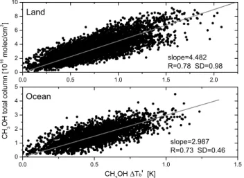
columns, is performed based on the retrievals in the selected regions and dates described in Table 1. Only retrievals re-sults with a DOFS higher than 0.75 and a RMS of the resid-ual lower than 4 × 10⁻⁶W/(m2sr m−1) are taken into ac-count. This translates to a total of 5147 and 2849 observa-tions above land and oceans, respectively. The correspond-ing scatter plots are shown in Fig. 5. In both cases, a linear fit shows good correlation coefficient (about 0.75). The slope for the retrievals over land is found to be much larger than
Fig. 5. Correlation between the retrieved total columns of methanol
and the corresponding 1Tbfor various regions (corrected for O3
and H2O dependency, see text for details). The conversion factors are given by the slopes of the linear fit (gray curve) separated for re-trievals above land (Top panel) and above ocean (Bottom panel). More details about the selected regions for the retrievals can be found in Table 1.
over oceans. Two different conversion factors are therefore used and applied to the 1T0
bcalculated globally: CCHland 3OH=4.482 × 1T 0 b (3) CCHocean 3OH=2.987 × 1T 0 b (4)
where the CH3OH total columns (CCH3OH) are expressed in 1016molec cm−2. Due to its noise, the minimum methanol total column which can be detected by IASI has been eval-uated from simulations using the 1976 US standard atmo-sphere to be about 1.60 × 10¹⁶molec cm−2. It is important to note that for the derivation of the global distributions, only cloud free measurements recorded during daytime were taken into account. This is justified because daytime mea-surements are generally characterized by a positive thermal contrast and are therefore more sensitive to the lower tropo-sphere.
3.2 Global distributions
The method proposed above allows to derive the first global distributions of methanol from IASI. In order to shed light onto seasonal variations, the four seasons have been differ-entiated as follows: DJF (December 2008, January 2009 and February 2009), MAM (March, April and May), JJA (June, July and August) and SON (September, October and Novem-ber). The resulting distributions averaged on a 0.5◦×0.5◦ grid are shown in Fig. 6. Note that measurements above sand surfaces, which causes erroneous high CH3OH
concentra-tions due to spectrally resolved surface emissivity (Wilber et al., 1999) have also been discarded.
Figure 6 shows large seasonal variations in the methanol columns. Higher concentrations are found in the north-ern hemisphere during spring and summer (up to 4 × 10¹⁶molec cm−2 in Central and Northern Asia) when veg-etation is growing. In the Southern Hemisphere, the high-est concentrations are found during the dry season (SON) and may be related to biomass burning. CH3OH is also
ob-served over oceans (with values around 2×10¹⁶molec cm−2) mostly between Africa and South America but also in the whole Northern hemisphere in spring and summertime. The presence of CH3OH in remote oceanic regions is probably
largely due to transport of continental emissions although oceanic emissions (Millet et al., 2008a) and the ubiquitous methane oxidation might also contribute. Methanol total columns range from about 0.01×10¹⁶molec cm−2above sea surfaces to 5.40 × 10¹⁶molec cm−2over large emission
re-gions.
During the northern hemispheric winter (DJF), methanol hot spots of low intensity are found in the Southern Hemi-sphere (South America, South Africa and Western Australia) above vegetated areas where CH3OH emissions may be
re-lated to plant growth. When comparing the distribution with AATSR (Arino et al., 2005) fire count maps, we find a high degree of coincidence in Africa between 5 and 15◦N, suggesting a possible biomass burning contribution. Dur-ing sprDur-ingtime (MAM), this specific region is subject to en-hanced CH3OH columns which is possibly due to an
in-crease in the fire numbers and intensities. Strong enhance-ments are also observed over India and to a lesser extent over Burma, Manchuria and Mexico, which can be at least partly related to biomass burning. In contrast, biomass burning is unlikely to be a dominant source in the Northern Hemi-sphere except in some regions (Kazakhstan, East Russia, Alaska) during JJA. It can be seen that CH3OH
concentra-tions are progressively increasing from winter (DJF) to sum-mertime (JJA). This can be explained by the seasonal cycle of the vegetation source which presents a maximum in late spring (Schade and Goldstein, 2006; Rinsland et al., 2009). During fall (SON), CH3OH concentrations decrease again
in the Northern Hemisphere and increase in the Southern Hemisphere. Again, biomass burning is likely responsible for the strong enhancements in South America, Congo and Northern Australia.
Although biomass burning is assumed to be a weak emis-sion source of methanol (accounting for less than 5% of to-tal emissions according to current inventories Jacob et al., 2005), the main hot spots in the global distributions could possibly be related to fires. This could be caused by the fact that methanol emitted by fire events is usually transported higher in the troposphere where the IASI sensitivity is larger or by the fact that a better sensitivity near the surface is in-duced because of higher surface temperatures for burning ar-eas. This is consistent with the fact that biomass burning has been found to be a significant source of methanol in the up-per troposphere (Dufour et al., 2007). The assimilation of
Fig. 6. Seasonal distributions of methanol total columns for the year 2009. The white areas correspond to a filter for sandy scenes where
emissivity is uncertain.
IASI data into models should help determining the respec-tive contributions of biogenic and fire emissions to the global methanol budget.
3.3 Error assessment
One of the disadvantages of the method described above is that it does not provide an estimate of the errors associated with the retrieved total columns. Because we are deriving the CH3OH columns from a weak signal, the associated error is
expected to be quite large. An estimate of the error on the CH3OH columns derived from IASI can be based on forward
simulations. For this purpose, we used a large set of different atmospheres compiled in an ECMWF database (Chevallier, 2001). Different input profiles are used for CH3OH,
corre-sponding to the different continental profiles taken from the IMAGESv2 model. The total columns used as input for the simulations are then compared to those retrieved from the simulated spectra using the same method as described above. The difference between the two columns gives a fair estimate of the absolute column errors. We do not expect these errors to be systematic on a global yearly scale but they cannot be excluded in particular circumstances such as in the presence of extreme values of ozone or water vapor.
It turns out that this absolute difference increases when the amount of CH3OH in the boundary layer (between the
surface and 3 km height) increases. It follows that the high concentrations of methanol in the boundary layer (close to
the emission sources) will not be well reproduced by the
1Tb method. This is consistent with the averaging kernel
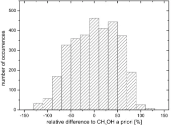
shape and the well known limited sensitivity of the infrared measurements toward low altitudes. Figure 7 shows the his-togram of the relative difference between the total columns used as input in the forward simulations and the calculated ones. Negative differences imply that the retrieved total col-umn from 1Tbis lower than the a priori value. Moreover,
dif-ferences lower than −100% are found but correspond only to methanol total columns which are below the detection limit of IASI (i.e. 1.60 × 10¹⁶molec cm−2). The distribution is similar to a normal distribution with a mean very close to zero (0.6%). The standard deviation (48.9%) provides our best estimate of the relative error on the retrieved methanol total column. This value is, however, clearly a lower bound for regions located close to emission sources and with low thermal contrast. In these regions, based on our analysis, er-rors as high as 100% are likely.
4 Formic acid retrieval and distributions 4.1 Retrieval settings and errors
In the case of formic acid, the target channel for brightness temperature has been chosen in the Q-branch at 1105.0 cm−1 which is the strongest absorption feature detectable in the IASI spectrum. The reference channels were chosen on both
Fig. 7. Histogram of the relative differences between the simulated
CH3OH total columns and the total columns derived from the 1Tb calculation.
sides at 1103.0 and 1109.0 cm−1. The 1Tbvalues computed
globally over one year range from about 0 to 5 K. As there exist large uncertainties on the vertical profile of formic acid, we have chosen here to rely on a composite vertical profile for the a priori. It was built from aircraft measurements for the low and free troposphere and from ACE-FTS for the up-per troposphere. The a priori profile is an average of profiles collected over the USA (25–55◦N, 230–290◦E) including (i) aircraft data from the INTEX-B C-130 campaign in April and May 2006 (Kleb et al., 2011) between 0–5 km, (ii) the arithmetic mean between INTEX-B data and ACE-FTS data (Abad et al., 2009) measured from March to May for alti-tudes between 6 and 8 km, (iii) and an averaged ACE-FTS profile between 9 and 11 km. The resulting profile, illustrated in Fig. 8, has a surface mixing ratio of about 750 pptv, which smoothly decreases as the altitude increases, down to less than 100 pptv above 7 km. Concentration above 11 km have been linearly extrapolated up to 20 km.
As in the case of methanol, conversion factors between the 1Tband the HCOOH total columns were tentatively
de-rived based on OEM retrievals in selected regions around the world. Because of the weak signal and the presence of water vapor interferences, the retrievals are unstable and lead to large errors. Forward simulations using the ECMWF database and varying the HCOOH concentrations (by scal-ing the profile, resultscal-ing in a variability of about 350%) were conducted to compute the relative difference between the true columns (input of the forward model) and those retrieved from the 1Tb. Figure 9 illustrates in gray the histogram of
these relative differences. The mode of the differences is lo-cated at about 60.0% suggesting a strong bias between the calculated and simulated total columns. Therefore, an alter-native method has been used to derive the conversion factor between the 1Tband the total columns. Relying only on the
Fig. 8. HCOOH a priori profile derived from the combined aircraft
and ACE measurements. See text for details.
Fig. 9. Histograms of the relative differences between the
simu-lated total columns of HCOOH and the HCOOH total columns ob-tained from brightness temperature differences. The gray histogram is derived from the conversion which uses OEM retrievals and the black one corresponds to the conversion obtained with simulated data. The latter, which is much less biased is used to obtain the global distributions (see Sect. 4.2).
forward calculations, it minimizes also the dependence upon the water vapor content (CH2Oexpressed in molec cm
−2) and
accounts for the varying sensitivity of the measurement to the local thermal contrast (τ ). The following equation is used
CHCOOH=
1Tb−b1τ −b2τ CH2O−c1CH2O−c2 a1τ +a2τ CH2O
(5)
with the parameters:
a1=0.024, a2=4 × 10⁻²⁶,
b1=0.005, b2=1 × 10⁻²⁶,
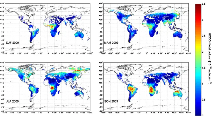
Fig. 10. Seasonal distributions of formic acid total columns for the year 2009. Only cloud free observations recorded during daytime above
continents along with a thermal contrast higher than 5 K were considered.
and where HCOOH total columns (CHCOOH) are expressed in
1016molec cm−2. The thermal contrast τ corresponds to the difference between the surface temperature and the air tem-perature at the first retrieved altitude level, located at about 100 m (both included in the IASI level 2 data). This mapping of 1Tb onto total columns of HCOOH provides much
bet-ter results. However a significant dependency on the thermal contrast remains, with lower errors found for higher thermal contrast values. We have chosen to consider only the cases for which the thermal contrast is higher than 5 K. This con-servative criterion excludes all retrievals above oceans. The resulting histogram of the relative differences between the simulated and calculated HCOOH total columns is shown in black on Fig. 9. It is similar to a normal distribution, with its mean being equal to −0.8%. Our estimation of the error on the formic acid total column is given by the standard deviation of the differences, which is about 60%. This error is only slightly higher than the error found for the CH3OH columns, but only applies here to favorable
situa-tions with large thermal contrast. Moreover, in the same way as methanol, the negative differences lower than −100% cor-respond only to HCOOH total columns which are below the detection limit of IASI (and has been evaluated to be about 0.60 × 10¹⁶molec cm−2).
This retrieval approach does not provide information about the vertical sensitivity of the formic acid total column. How-ever, the limited set of full profile retrievals performed give a maximum sensitivity between 4 and 14 km.
4.2 Global distributions
The global distributions of formic acid for the four seasons are illustrated in Fig. 10, on a 0.5◦×0.5◦averaged grid. Only cloud free observations recorded during daytime and with a thermal contrast higher or equal to 5 K were taken into account. The latter constraint removes unfortunately many observations at high latitudes (no observations above about 45◦N in winter and about 65◦N during summer). Grid points which include less than ten HCOOH measurements were also filtered out. As for CH3OH, clear seasonal variations are
observed. The retrieved HCOOH total columns range from background values of less than 0.5 × 10¹⁶molec cm−2above Europe and North America to 5×10¹⁶molec cm−2above fire events, mainly during summer 2009 in Africa. These high formic acid total columns in fire plumes are in good agree-ment with the values reported by Coheur et al. (2009) and Worden et al. (1997) if we account for the factor 2 resulting from the use of the improved line parameters (Vander Auw-era et al., 2007).
The 2009 northern hemispheric winter season (DJF) shows the lowest number of observations. Comparing with AATSR fire counts during that period, we found that en-hancements of HCOOH in the western-central region of Africa and to a lesser extent in South America might be partly due to biomass burning. During spring (MAM), we ob-serve a decrease in the HCOOH total columns above Africa and South America together with a fire count decrease.
High concentrations are also found in Asia (India, Burma and Manchuria) which are well correlated with CH3OH
hot spots. The peak of the biomass burning season in South America and Southern Africa happens usually around August–September whereas in Australia most of the burn-ing occurs around October–November (Gloudemans et al., 2006). Together with the minimal washout of HCOOH oc-curring during the dry season, it probably largely explains the high HCOOH total columns observed during JJA above Congo and Brazil as well as in Northern Australia during the SON period. The overall increase of formic acid in the Northern Hemisphere during JJA is likely caused by the sea-sonality of its biogenic emissions. However, according to the AATSR fire count distributions, some regions with large HCOOH columns may be associated with boreal fires such as in Eastern Russia and in Alaska. Finally, the very widespread hot spots found during SON above Amazonia and Central Africa do not seem to be only related to fires and very likely points also to biogenic emissions of either HCOOH or HCOOH precursors. Throughout the year (MAM through SON, no available data for DJF), large HCOOH columns are observed in Eastern China which may partly be due to anthropogenic activities. Several common patterns are also found in the distributions of HCOOH and CH3OH columns,
probably due to their common emission sources (such as biomass burning and plant growth). Also note that the sea-sonality observed here is in good agreement with that re-ported from ACE-FTS (Abad et al., 2009) and from MIPAS (Grutter et al., 2010).
5 Seasonal variations in relation to biomass burning
In this section we compare the 2009 time series of methanol, formic acid and carbon monoxide for three selected regions subject to biomass burning. The vertical sensitivity profiles of IASI for these three species are all maximum in the free troposphere, i.e. between 4 to 14 km, 6 to 10 km and between 3 to 12 km for HCOOH, CH3OH and CO total columns,
spectively. The comparisons are therefore most likely to re-flect similarities/differences in the free tropospheric columns but fine structures in the respective profiles could be missed. Monthly mean total columns of methanol and formic acid are shown in Fig. 11 together with the total columns of car-bon monoxide and the AATSR fire counts for three 10◦×10◦ regions located in Brazil (15 − 5◦S, 60 − 50◦W), Congo (15−5◦S, 20−30◦E) and South-East Asia (20−30◦N, 95− 105◦E). For each regions, the time series of CO, CH
3OH
and HCOOH are similar. An increase in the total columns is observed for the three species just after the month with the maximum fire counts. This delay may be induced by the fact that the probed air masses are located in the free tro-posphere and are therefore subject to some transport which could result in the spreading of the species or the spatial dis-placement of the maxima. The highest number of fires
(ex-Fig. 11. Time series of methanol (green curve), formic acid (blue
curve) and carbon monoxide (black curve) monthly mean total columns for three different areas associated with biomass burn-ing (Brazil, Congo and SE Asia). Carbon monoxide total columns where divided by 100 for comparison. The left scale and gray curves correspond to the sum of the AATSR fire counts for each months.
ceeding 700) is found above Congo where methanol, formic acid and carbon monoxide reach high values, with increases of about 1.6 × 10162.5 × 1016and 1.4 × 10¹⁸molec cm−2in comparison with their mean total column between January and June, respectively. In each cases, the CH3OH maximum
lasts longer than for CO or HCOOH. This cannot be ex-plained by its lifetime which is similar to formic acid in the free troposphere (about one week) but suggests an additional source or transport to this region. Overall higher concentra-tions of CH3OH found above Brazil and Congo may also be
due to the larger biogenic source in these regions.
In addition to looking into correlations regionally, prelim-inary global analyses were carried out. Linear correlations (R2=0.7) between CH3OH and HCOOH were found during
the DJF and SON periods highlighting specific emissions or fate of these two species.
6 Conclusions and perspectives
In this study, we have retrieved methanol and formic acid from the data provided by the IASI sounder. Using a radi-ance indexing method and the calculation of brightness tem-perature differences, first global distributions are computed. They are provided as total columns, after careful conversion of the brightness temperature differences. The conversion has been achieved based on a set of retrievals in selected re-gions for methanol and on forward simulations for formic
acid. Taking full advantage of the IASI spatial and temporal coverage, unprecedented information on the location and ori-gin of sources have been acquired.
The simple retrieval method used here does not allow the determination of individual error for each observations. We have estimated, using a large set of representative forward calculation, global errors of about typically 50% and 60% for the methanol and formic acid total columns, respectively. Al-though these errors are significant, this robust method takes advantage of the very large number of IASI measurements at low computational cost. In this way, we provide global observations for these two volatile organic compounds.
The global distributions shown in this study highlight strong seasonal variations for methanol and formic acid with maximum total column values evaluated at 5.4 and 5.0 × 10¹⁶molec cm−2, respectively. The strong
enhance-ments seen in the global maps might be largely attributed to biomass burning (mostly in tropical regions). The main seasonal patterns, especially at mid-latitudes where we find higher columns in spring and summer, might be explained by variations in biogenic emissions and increased plant growth. Anthropogenic emissions could not been clearly identified in these distributions.
Time series of methanol, formic acid, carbon monoxide and AATSR fire counts were also compared and found to be fairly well correlated for three different regions (Congo, Brazil and South-East Asia) where biomass burning is their likely common source.
It is anticipated that the assimilation of these data in a global chemistry model will help to improve the determi-nation of the emission fluxes for these two species. Mean averaging kernels for methanol (differentiated for land and ocean) are provided in order to account for the vertical sen-sitivity of the measurements.
Acknowledgements. IASI has been developed and built under the
responsibility of the Centre National d’Etudes Spatiales (CNES, France). It is flown onboard the MetOp satellites as part of the EUMETSAT Polar System. The IASI L1 data are received through the EUMETCast near real time data distribution service. The research in Belgium was funded by the “Communaut´e Franc¸aise de Belgique – Actions de Recherche Concert´ees”, the Fonds National de la Recherche Scientifique (FRS-FNRS F.4511.08), the Belgian Science Policy Office and the European Space Agency (ESA-Prodex C90-327). The ACE mission is funded primarily by the Canadian Space Agency.
Edited by: C. McNeil
References
Abad, G. G., Bernath, P. F., Boone, C. D., McLeod, S. D., Manney, G. L., and Toon, G. C.: Global distribution of upper tropospheric formic acid from the ACE-FTS, Atmos. Chem. Phys., 9, 8039– 8047, doi:10.5194/acp-9-8039-2009, 2009.
Arino, O., Plummer, S., and Defrenne, D.: Fire disturbance: the ten years time series of the ATSR World Fire Atlas, in: ATSR Workshop, 26–30, 2005.
Arlander, D., Cronn, D., Farmer, J., Menzia, F., and Westberg, H.: Gaseous oxygenated hydrocarbons in the remote marine tropo-sphere, J. Geophys. Res., 95, 16391–16403, 1990.
Atkinson, R.: Kinetics and mechanisms of the gas-phase reactions of the hydroxyl radical with organic compounds under atmo-spheric conditions, Chem. Rev., 86, 69–201, 1986.
Atkinson, R. and Arey, J.: Atmospheric degradation of volatile or-ganic compounds, Chem. Rev., 103, 4605–4638, 2003.
Beer, R., Shephard, M., Kulawik, S., Clough, S., Eldering, A., Bowman, K., Sander, S., Fisher, B., Payne, V., Luo, M., Os-terman, G., and Worden, J.: First satellite observations of lower tropospheric ammonia and methanol, Geophys. Res. Lett., 35, L09801, doi:10.1029/2008GL033642, 2008.
Boynard, A., Clerbaux, C., Coheur, P.-F., Hurtmans, D., Turquety, S., George, M., Hadji-Lazaro, J., Keim, C., and Mayer-Arnek, J.: Measurements of total and tropospheric ozone from the IASI instrument: comparison with satellite and ozone sonde observa-tions, Atmos. Chem. Phys., 9, 6255–6271, doi:10.5194/acp-9-6255-2009, 2009.
Brunner, A., Ammann, C., Neftel, A., and Spirig, C.: Methanol ex-change between grassland and the atmosphere, Biogeosciences, 4, 395–410, doi:10.5194/bg-4-395-2007, 2007.
Butkovskaya, N., Pouvesle, N., Kukui, A., and Le Bras, G.: Mech-anism of the OH-Initiated Oxidation of Glycolaldehyde over the Temperature Range 233–296 K, J. Phys. Chem. A, 110, 13492– 13499, 2006a.
Butkovskaya, N., Pouvesle, N., Kukui, A., Mu, Y., and Le Bras, G.: Mechanism of the OH-Initiated Oxidation of Hydroxyace-tone over the Temperature Range 236-298 K, J. Phys. Chem. A, 110, 6833–6843, 2006b.
Chameides, W. and Davis, D.: Aqueous-phase source of formic acid in clouds, Nature, 304, 427–429, 1983.
Chance, K., Palmer, P. I., Spurr, R. J., Martin, R., Kurosu, T. P., and Jacob, D. J.: Satellite observations of formaldehyde over North America from GOME, Geophys. Res. Lett., 27, 3461– 3464, 2000.
Charlson, R., Lovelock, J., Andreae, M., and Warren, S.: Oceanic phytoplankton, atmospheric sulphur, cloud albedo and climate, Nature, 326, 16, 1987.
Chevallier, F.: Sampled databases of 60-level atmospheric profiles from the ECMWF analysis, Tech. Rep. Research Report No. 4, Eumetsat/ECMWF SAF Programme, 2001.
Clarisse, L., Coheur, P.-F., Prata, A. J., Hurtmans, D., Razavi, A., Hadji-Lazaro, J., Clerbaux, C., and Phulpin, T.: Tracking and quantifying volcanic SO2 with IASI, the September 2007
eruption at Jebel-at-Tair, Atmos. Chem. Phys., 8, 7723–7734, doi:10.5194/acp-8-7723-2008, 2008.
Clarisse, L., Clerbaux, C., Dentener, F., Hurtmans, D., and Co-heur, P.-F.: Global ammonia distribution derived from infrared satellite observations, Nat. Geosci., 2, 479–483, doi:doi:10.1038/ ngeo551, 2009.
Clarisse, L., Shephard, M., Dentener, F., Hurtmans, D., Cady-Pereira, K., Karagulian, F., Van Damme, M., Clerbaux, C., and Coheur, P.-F.: Satellite monitoring of ammonia: A case study of the San Joaquin Valley, J. Geophys. Res., 115, D13302, doi:10.1029/2009JD013291, 2010.
Clerbaux, C., Boynard, A., Clarisse, L., George, M., Hadji-Lazaro, J., Hurtmans, D., Herbin, H., Pommier, M., Razavi, A., Turquety, S., Wespes, C., and Coheur, P.-F.: Monitoring of atmospheric composition using the thermal infrared IASI/METOP sounder, Atmos. Chem. Phys., 9, 6041–6054, doi:10.5194/acp-9-6041-2009, 2009.
Coheur, P.-F., Barret, B., Turquety, S., Hurtmans, D., Hadji-Lazaro, J., and Clerbaux, C.: Retrieval and characterization of ozone ver-tical profiles from a thermal infrared nadir sounder, J. Geophys. Res., 5, 4599–4639, 2005.
Coheur, P., Herbin, H., Clerbaux, C., Hurtmans, D., Wespes, C., Carleer, M., Turquety, S., Rinsland, C., Remedios, J., Hauglus-taine, D., Boone, C., and P.F., B.: ACE-FTS observation of a young biomass burning plume: first reported measurements of C2H4, C3H6O, H2CO and PAN by infrared occultation from
space, Atmos. Chem. Phys., 7, 5437–5446, doi:10.5194/acp-7-5437-2007, 2007.
Coheur, P.-F., Clarisse, L., Turquety, S., Hurtmans, D., and Cler-baux, C.: IASI measurements of reactive trace species in biomass burning plumes, Atmos. Chem. Phys., 9, 5655–5667, doi:10.5194/acp-9-5655-2009, 2009.
De Smedt, I., M¨uller, J., Stavrakou, T., van der A, R., Eskes, H., and Van Roozendael, M.: Twelve years of global obser-vations of formaldehyde in the troposphere using GOME and SCIAMACHY sensors, Atmos. Chem. Phys., 8, 4947–4963, doi:10.5194/acp-8-4947-2008, 2008.
Dufour, G., Boone, C. D., Rinsland, C. P., and Bernath, P. F.: First space-borne measurements of methanol inside aged south-ern tropical to mid-latitude biomass burning plumes using the ACE-FTS instrument, Atmos. Chem. Phys., 6, 3463–3470, doi:10.5194/acp-6-3463-2006, 2006.
Dufour, G., Szopa, S., Hauglustaine, D. A., Boone, C. D., Rins-land, C. P., and Bernath, P. F.: The influence of biogenic emis-sions on upper-tropospheric methanol as revealed from space, Atmos. Chem. Phys., 7, 6119–6129, doi:10.5194/acp-7-6119-2007, 2007.
Eerdekens, G., Ganzeveld, L., Vil´a-Guerau de Arellano, J., Kl¨upfel, T., Sinha, V., Yassaa, N., Williams, J., Harder, H., Kubistin, D., Martinez, M., and Lelieveld, J.: Flux estimates of isoprene, methanol and acetone from airborne PTR-MS measurements over the tropical rainforest during the GABRIEL 2005 campaign, Atmos. Chem. Phys., 9, 4207–4227, doi:10.5194/acp-9-4207-2009, 2009.
Feingold, G., Eberhard, W., Veron, D., and Previdi, M.: First measurements of the Twomey indirect effect using ground-based remote sensors, Geophys. Res. Lett., 30, 1287, doi:10.1029/2002GL016633, 2003.
Filella, I. and Pen¸uelas, J.: Daily, weekly, and seasonal time courses of VOC concentrations in a semi-urban area near Barcelona, At-mos. Environ., 40, 7752–7769, 2006.
Fischer, H., de Reus, M., Traub, M., Williams, J., Lelieveld, J., de Gouw, J., Warneke, C., Schlager, H., Minikin, A., Scheele, R., and Siegmund, P.: Deep convective injection of boundary layer air into the lowermost stratosphere at midlatitudes, Atmos.
Chem. Phys., 3, 739–745, doi:10.5194/acp-3-739-2003, 2003. Fu, T., Jacob, D., Palmer, P., Chance, K., Wang, Y., Barletta, B.,
Blake, D., Stanton, J., and Pilling, M.: Space-based formalde-hyde measurements as constraints on volatile organic compound emissions in east and south Asia and implications for ozone, J. Geophys. Res., 112, D06312, doi:10.1029/2006JD007853, 2007. Galbally, I. and Kirstine, W.: The production of methanol by flow-ering plants and the global cycle of methanol, J. Atmos. Chem., 43, 195–229, 2002.
George, M., Clerbaux, C., Coheur, P.-F., Hadji-Lazaro, J., Hurt-mans, D., Pommier, M., Turquety, S., Edwards, D., Worden, H., Luo, M., Rinsland, C. P., and Barnet, C.: Carbon monoxide dis-tributions from the IASI/METOP mission : evaluation with other spaceborne remote sensors, Atmos. Chem. Phys., 9, 8317–8330, doi:10.5194/acp-9-8317-2009, 2009.
Glatthor, N., Von Clarmann, T., Fischer, H., Funke, B., Grabowski, U., H¨opfner, M., Kellmann, S., Kiefer, M., Linden, A., Milz, M., et al.: Global peroxyacetyl nitrate(PAN) retrieval in the up-per troposphere from limb emission spectra of the Michelson Interferometer for Passive Atmospheric Sounding (MIPAS), At-mos. Chem. Phys., 7, 2775–2787, doi:10.5194/acp-7-2775-2007, 2007.
Glatthor, N., Von Clarmann, T., Stiller, G., Funke, B., Koukouli, M., Fischer, H., Grabowski, U., H¨opfner, M., Kellmann, S., and Linden, A.: Large-scale upper tropospheric pollution observed by MIPAS HCN and C2H6global distributions, Atmos. Chem. Phys., 9, 9619–9634, doi:10.5194/acp-9-9619-2009, 2009. Gloudemans, A., Krol, M., Meirink, J., De Laat, A., Van der Werf,
G., Schrijver, H., Van den Broek, M., and Aben, I.: Evidence for long-range transport of carbon monoxide in the Southern Hemi-sphere from SCIAMACHY observations, Geophys. Res. Lett., 33, 16807, doi:10.1029/2006GL026804, 2006.
Goldman, A., Murcray, F., Murcray, D., and Rinsland, C.: A search for formic acid in the upper troposphere: A tentative identifi-cation of the 1105 cm−1 ν6 band Q-branch in highresolution
balloon-borne solar absorption spectra, Geophys. Res. Lett, 11, 307–310, 1984.
Goode, J., Yokelson, R., Ward, D., Susott, R., Babbitt, R., Davies, M., and Hao, W.: Measurements of excess O3, CO2, CO, CH4,
C2H4, C2H2, HCN, NO, NH3, HCOOH, CH3COOH, HCHO,
and CH3OH in 1997 Alaskan biomass burning plumes by
air-borne Fourier transform infrared spectroscopy (AFTIR), J. Geo-phys. Res., 105, 22147, doi:10.1029/2000JD900287, 2000. Graedel, T. and Eisner, T.: Atmospheric formic acid from formicine
ants: a preliminary assessment, Tellus B, 40, 335–339, 1988. Granby, K., Christensen, C., and Lohse, C.: Urban and semi-rural
observations of carboxylic acids and carbonyls, Atmos. Environ., 31, 1403–1415, 1997.
Grosjean, D.: Organic acids in southern California air: ambient concentrations, mobile source emissions, in situ formation and removal processes, Environ. Sci. Technol., 23, 1506–1514, 1989. Grosjean, D.: Formic acid and acetic acid measurements during the Southern California Air Quality Study, Atmos. Environ., 24, 2699–2702, 1990.
Grutter, M., Glatthor, N., Stiller, G., Fischer, H., Grabowski, U., H¨opfner, M., Kellmann, S., Linden, A., and von Clarmann, T.: Global distribution and variability of formic acid as ob-served by MIPAS-ENVISAT, J. Geophys. Res., 115, D10303, doi:10.1029/2009JD012980, 2010.
Harley, P., Greenberg, J., Niinemets, U., and Guenther, A.: Envi-ronmental controls over methanol emission from leaves, Biogeo-sciences, 4, 1083–1099, doi:10.5194/bg-4-1083-2007, 2007. Hartmann, W., Santana, M., Hermoso, M., Andreae, M., and
San-hueza, E.: Diurnal cycles of formic and acetic acids in the north-ern part of the Guayana shield, Venezuela, J. Atmos. Chem., 13, 63–72, 1991.
Heald, C., Henze, D., Horowitz, L., Feddema, J., Lamarque, J., Guenther, A., Hess, P., Vitt, F., Seinfeld, J., Goldstein, A., and Fung, I.: Predicted change in global secondary or-ganic aerosol concentrations in response to future climate, emis-sions, and land use change, J. Geophys. Res., 113, D05211, doi:10.1029/2007JD009092, 2008.
Heikes, B., Chang, W., Pilson, M., Swift, E., Singh, H., Guen-ther, A., Jacob, D., Field, B., Fall, R., Riemer, D., et al.: At-mospheric methanol budget and ocean implication, Global Bio-geochem. Cy., 16, 1133, doi:10.1029/2002GB001895, 2002. Helas, G., Bingemer, H., and Andrea, M.: Organic acids over
equa-torial Africa – Results from DECAFE 88, J. Geophys. Res., 97, 6187–6193, 1992.
Herbin, H., Hurtmans, D., Clarisse, L., Turquety, S., Clerbaux, C., Rinsland, C., Boone, C., Bernath, P., and Coheur, P.: Distributions and seasonal variations of tropospheric ethene (C2H4) from Atmospheric Chemistry Experiment (ACE-FTS)
solar occultation spectra, Geophys. Res. Lett., 36, L04801, doi:10.1029/2008GL036338, 2009.
Hermans, I., M¨uller, J., Nguyen, T., Jacobs, P., and Peeters, J.: Kinetics of [alpha]-Hydroxy-alkylperoxyl Radicals in Oxidation Processes. HO2•-Initiated Oxidation of Ketones/Aldehydes near
the Tropopause, J. Phys. Chem., 109, 4303–4311, 2005. Herndon, S., Zahniser, M., Nelson Jr, D., Shorter, J., McManus, J.,
Jim´enez, R., Warneke, C., and de Gouw, J.: Airborne measure-ments of HCHO and HCOOH during the New England Air Qual-ity Study 2004 using a pulsed quantum cascade laser spectrome-ter, J. Geophys. Res., 112, D10S03, doi:10.1029/2006JD007600, 2007.
Holzinger, R., Williams, J., Salisbury, G., Kl¨upfel, T., De Reus, M., Traub, M., Crutzen, P., and Lelieveld, J.: Oxygenated compounds in aged biomass burning plumes over the East-ern Mediterranean: evidence for strong secondary production of methanol and acetone, Atmos. Chem. Phys., 4, 6321–6340, doi:10.5194/acp-4-6321-2005, 2005.
Houweling, S., Dentener, F., and Lelieveld, J.: The impact of non-methane hydrocarbon compounds on tropospheric photochem-istry, J. Geophys. Res., 103, 673–10, 1998.
Jacob, D.: Chemistry of OH in remote clouds and its role in the production of formic acid and peroxymonosulfate, J. Geophys. Res., 91, 9807–9826, 1986.
Jacob, D. and Wofsy, S.: Photochemistry of biogenic emissions over the Amazon forest, J. Geophys. Res., 93, 1477–1486, 1988. Jacob, D., Field, B., Li, Q., Blake, D., de Gouw, J., Warneke, C.,
Hansel, A., Wisthaler, A., Singh, H., and Guenther, A.: Global budget of methanol: Constraints from atmospheric observations, J. Geophys. Res., 110, D08303, doi:10.1029/2004JD005172, 2005.
Jaegl´e, L., Jacob, D., Brune, W., Faloona, I., Tan, D., Heikes, B., Kondo, Y., Sachse, G., Anderson, B., Gregory, G., Singh, H., Pueschel, R., Ferry, G., Blake, D., and Shetter, R. E.: Photo-chemistry of HOxin the upper troposphere at northern
midlati-tudes, Environ. Sci. Technol., 105(D3), 3877–3892, 2000. Jordan, C., Fitz, E., Hagan, T., Sive, B., Frinak, E., Haase, K.,
Cottrell, L., Buckley, S., and Talbot, R.: Long-term study of VOCs measured with PTR-MS at a rural site in New Hamp-shire with urban influences, Atmos. Chem. Phys., 9, 4677–4697, doi:10.5194/acp-9-4677-2009, 2009.
Karl, T., Guenther, A., Spirig, C., Hansel, A., and Fall, R.: Sea-sonal variation of biogenic VOC emissions above a mixed hard-wood forest in northern Michigan, Geophys. Res. Lett., 30, 2186, doi:10.1029/2003GL018432, 2003.
Karl, T., Harley, P., Guenther, A., Rasmussen, R., Baker, B., Jar-dine, K., and Nemitz, E.: The bi-directional exchange of oxy-genated VOCs between a loblolly pine (Pinus taeda) plantation and the atmosphere, Atmos. Chem. Phys., 5, 3015–3031, 2005, http://www.atmos-chem-phys.net/5/3015/2005/.
Karl, T., Guenther, A., Yokelson, R., Greenberg, J., Poto-snak, M., Blake, D., and Artaxo, P.: The tropical forest and fire emissions experiment: Emission, chemistry, and trans-port of biogenic volatile organic compounds in the lower at-mosphere over Amazonia, J. Geophys. Res., 112, D18302, doi:10.1029/2007JD008539, 2007.
Kawamura, K., Ng, L., and Kaplan, I.: Determination of organic acids (C1-C10) in the atmosphere, motor exhausts, and engine
oils, Environ. Sci. Technol., 19, 1082–1086, 1985.
Keene, W. and Galloway, J.: Organic acidity in precipitation of North America, Atmos. Environ., 18, 2491–2497, 1984. Keene, W. and Galloway, J.: The biogeochemical cycling of formic
and acetic acids through the troposphere: An overview of current understanding, Tellus B, 40, 322–334, 1988.
Khwaja, H.: Atmospheric concentrations of carboxylic acids and related compounds at a semiurban site, Atmos. Environ., 29, 127–139, 1995.
Kleb, M. M., Chen, G., Crawford, J. H., Flocke, F. M., and Brown, C. C.: An overview of measurement comparisons from the INTEX-B/MILAGRO airborne field campaign, Atmos. Meas. Tech., 4, 9–27, doi:10.5194/amt-4-9-2011, 2011.
MacDonald, R. and Fall, R.: Detection of substantial emissions of methanol from plants to the atmosphere, Atmos. Environ., 27, 1709–1713, 1993.
Martin, R., Westberg, H., Allwine, E., Ashman, L., Farmer, J., and Lamb, B.: Measurement of isoprene and its atmospheric oxida-tion products in a central Pennsylvania deciduous forest, J. At-mos. Chem., 13, 1–32, 1991.
Meinshausen, M., Hare, B., Wigley, T., Van Vuuren, D., Den Elzen, M., and Swart, R.: Multi-gas emissions pathways to meet climate targets, Clim. Change, 75, 151–194, 2006.
Millet, D., Jacob, D., Custer, T., de Gouw, J., Goldstein, A., Karl, T., Singh, H., Sive, B., Talbot, R., Warneke, C., and Williams, J.: New constraints on terrestrial and oceanic sources of atmospheric methanol, Atmos. Chem. Phys., 8, 6887–6905, doi:10.5194/acp-8-6887-2008, 2008a.
Millet, D., Jacob, D., Folkert Boersma, K., Fu, T.-M., Kurosu, T., Chance, K., Heald, C., and Guenther, A.: Spatial distribu-tion of isoprene emissions from North America derived from formaldehyde column measurements by the OMI satellite sensor, J. Geophys. Res., 113, D02307, doi:doi:10.1029/2007JD008950, 2008b.
Monks, P.: Gas-phase radical chemistry in the troposphere, Chem. Soc. Rev., 34, 376–395, 2005.