Effect of image scaling and segmentation
in digital rock characterisation
The MIT Faculty has made this article openly available. Please share
how this access benefits you. Your story matters.
Citation
Jones, B. D., and Y. T. Feng. “Effect of Image Scaling and
Segmentation in Digital Rock Characterisation.” Computational
Particle Mechanics 3, no. 2 (October 19, 2015): 201–213.
As Published
http://dx.doi.org/10.1007/s40571-015-0077-0
Publisher
Springer International Publishing
Version
Author's final manuscript
Citable link
http://hdl.handle.net/1721.1/103309
Terms of Use
Article is made available in accordance with the publisher's
policy and may be subject to US copyright law. Please refer to the
publisher's site for terms of use.
Effect of Image Scaling and Segmentation in Digital
Rock Characterisation
B. D. Jones · Y. T. Feng
Received: date / Accepted: date
Abstract Digital material characterisation from microstructural geometry is
an emerging field in computer simulation. For permeability characterisation, a variety of studies exist where the lattice Boltzmann method has been used in conjunction with CT imaging to simulate fluid flow through microscopic rock pores. Whilst these previous works show that the technique is applicable, the use of binary image segmentation and the bounceback boundary condition results in a loss of grain surface definition when the modelled geometry is compared to the original CT image.
We apply the immersed moving boundary condition of Noble & Torczyn-ski as a partial bounceback boundary condition which may be used to better represent the geometric definition provided by a CT image. The immersed moving boundary condition is validated against published work on idealised porous geometries in both 2D and 3D. Following this, greyscale image seg-mentation is applied to a CT image of Diemelstadt sandstone. By varying the mapping of CT voxel densities to lattice sites, it is shown that binary image segmentation may underestimate the true permeability of the sample. A CUDA-C based code, LBM-C, was developed specifically for this work and leverages GPU hardware in order to carry out computations.
Keywords Lattice Boltzmann· CT Imaging · Permeability · GPU Computing
B. D. Jones
Massachusetts Institute of Technology 77 Massachusetts Ave., Cambridge MA 02139
USA
E-mail: [email protected] Y. T. Feng
College of Engineering, Swansea University Singleton Park, Swansea
SA2 8PP UK
1 Introduction
Computational material characterisation represents a useful tool in a number of industries. From a single digital sample multiple tests may be carried out. Though the generation of such a digital sample may be destructive, the indi-vidual tests are not. This work is concerned with computational permeability analysis of rock material, where the proposed methodology involves the use of the lattice Boltzmann method to simulate the flow of fluid through the microstructural geometry of rock material.
Various authors have used the lattice Boltzmann method (LBM) to deter-mine, computationally, the permeability of rock material [1–4]. In these works computed tomography (CT) imaging is used to gain an approximate represen-tation of the micro-structure of a rock sample. Though the produced image is greyscale, these authors apply binary image segmentation to the images to separate them into regions representing solid and void space. This approach is attractive as it enables the use of the simple bounceback boundary condition to represent the porous geometry.
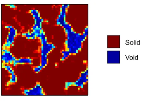
Solid Void
Fig. 1: CT Image Slice
A major drawback of binary image segmentation is that the definition of the solid/void interface provided by a CT image is lost in the process. CT images are not binary in nature, and are instead a grey-scale representation of the rock geometry. This is demonstrated in figure 1, where the bitmap shown is a slice of a typical CT image of Diemelstadt sandstone. Regions shown in red correspond to high density voxels, where blue regions correspond to low density voxels. Where the rock grains intersect a voxel, we observe a density intermediate to that of the void and solid regions.
In an attempt to better represent the geometric definition provided by CT imaging, Ahrenholz et al. [2] applied the marching cubes algorithm to define a boundary surface mesh of the porous geometry from the CT image data. They then applied an interpolated no slip boundary condition developed by
Ginzburg & d’Humi`eres [5]. Both determining the surface mesh, and voxelisa-tion of this mesh, are computavoxelisa-tionally expensive operavoxelisa-tions. Addivoxelisa-tionally, the resultant mesh is a smoothed representation of the solid surface boundary.
Once a CT image has been segmented, computational limitations may re-quire the image to be scaled so that the resulting flow model is computationally feasible. This is especially true on limited memory architectures such as GPU’s, where it may not be possible to fit a high resolution representative elementary volume on to a single graphics card. Using standard image scaling techniques, reducing the resolution of a CT image is straightforward. However, application of binary image segmentation to a scaled image will result in a further loss of geometric definition, causing significant changes in image porosity. If the greyscale definition of the image is preserved, the porosity of the image should at least remain constant through scaling. It is not clear however if consistent permeability results may be gained as the image is coarsened
In this work, we have used the Immersed Moving Boundary Condition (IMB) developed by Noble & Torczynski [6] to represent those voxels which appear to be intersected by the rock grains. We begin with an initial valida-tion of the IMB for permeability assessment of idealised porous geometries. Following this, we carry out permeability assessment on a Diemelstadt sand-stone sample. By varying the mapping of CT image data to model geometry, we demonstrate that the choice of image segmentation approach and scaling factor have a significant impact on the overall approximation of sample perme-ability. Following this, we look at the way in which permeability may vary due to flow regime in the porous sample. In order to expedite these computations, a CUDA-C based code, LBM-C, was developed to exploit the advantages offered by GPU hardware.
2 Methodology
In this work we use the lattice Boltzmann method to simulate the flow of fluid through porous geometries. In the section that follows, the lattice Boltzmann method and relevant boundary conditions is described. The use of the partial bounceback boundary condition is supported through validation with idealised porous geometries. Finally, the preprocessing and segmentation of a CT image for permeability analysis is discussed.
2.1 The Lattice Boltzmann Method
A review by Aidun & Clausen demonstrates that the LBM has found applica-tions in a variety of fields including, multiphase flow, particle suspensions, and microfluidic devices [7]. This flexibility has led to the methods popularity in modelling flow through porous media, where it has been applied by a number of authors [1, 2, 8, 9].
The LBM is derived from the Boltzmann equation [10], which describes the statistical likelihood that a particle exists with some momentum at any
given point in space and time. These origins set the LBM apart from con-temporary Finite Difference, Finite Volume, and Finite Element techniques which derive instead from the Navier-Stokes [11] set of equations. Despite the differing origins of the two approaches, it is possible to derive the full set of Navier-Stokes equations by applying the Chapman-Enskog expansion to the lattice Boltzmann equation [12]. We provide here a brief description of the method, a comprehensive review of the associated theory is provided by Chen & Doolen [13].
The LBM began as an extension to the family of methods known as the Lattice Gas Automata [14]. The LGA received much attention during the 80’s, especially for flows through complex geometries. An example of this is given by Rothman, who applied the LGA to flow through porous media [15].
The LGA typically operates on hexagonal lattice, due to the lack of ro-tational invariance in square lattice. The existence of particles at a lattice site, travelling in the direction parallel to a lattice link, was indicated with a boolean variable. As particles arrive at a lattice site, a simple collision process is carried out. Where the results produced from this algorithm demonstrate it’s ability to simulate the flow of fluids.
In an attempt to reduce the statistical noise present in LGA simulations, McNamara & Zanetti replaced the boolean particle populations in the LGA with real valued particle distribution functions [16]. Further efforts in method development focused on moving away from schemes developed for the LGA. Higuera & Jim´enez introduced the notion of a relaxation toward an equilib-rium state for particle collision [17]. Finally, in 1992, by using the simplified Bhatnagar-Gross-Krook (BGK) collision operator [18] both Qian et. al [19] and Chen et. al [20] independently developed the scheme which is now com-monly referred to as the BGK lattice Boltzmann method.
In comparison to classical continuum techniques, the LBM has two primary difference.
First, the LBM operates on a regular grid of computational cells. Using a regular grid avoids the complexities of generating body fitted meshes typically used with continuum methods. The use of a regular grid also simplifies the implementation of the method since the grid can be represented by a multidi-mensional array.
The second difference lies in the simple, local, nature of the lattice Boltz-mann equation. Solution calculation consists of a series of simple arithmetic operations involving no differential terms. The result of this is that an LBM code is relatively short when compared to a typical continuum based code. The LBM algorithm is also particularly well suited to parallel execution.
The standard BGK lattice Boltzmann equation is given by fi(x + ei∆t, t + ∆t)− fi(x, t) =
1 τ(f
eq
i (ρ, u)− fi(x, t)) (1)
in which the terms fi and f eq
i are particle and equilibrium distribution
position; ei are lattice vectors; ρ is macroscopic density; u is macroscopic
ve-locity; t is time, and ∆t is the time step. Further discussion on the lattice Boltzmann equation and associated variables is given by Feng et. al [21].
The lattice Boltzmann equation assumes that for an ensemble average of particles at a point in space, there exists some equilibrium state. While the equation encapsulates two processes, streaming and collision.
During the streaming step particle distribution functions propagate to ad-jacent lattice sites. During the collision step the set of particle distribution functions arriving at a lattice site are relaxed toward some equilibrium state. The strength of this relaxation process is defined by the relaxation time.
In the same year as the introduction of the BGK lattice Boltzmann method, d’Humi`eres proposed the generalized lattice Boltzmann method [22]. Also known as the Multiple Relaxation Time (MRT) method, this technique re-quires that particle collision occurs in moment space where a set of relax-ation times exist corresponding to each moment. This is as opposed to the single relaxation time used in equation (1). The primary advantage of the MRT method stems from these additional relaxation times. Hydrodynamic and non-hydrodynamic relaxation times may be set independently, and the non-hydrodynamics terms may be set to improve stability without affecting the hydrodynamic solution.
Pan et. al carried out a comparison of collision operators used in perme-ability approximation [23]. They applied both the MRT and BGK methods, in conjunction with a number of no-slip boundary conditions. Of most signif-icance is their observation that permeability non-physically varies with fluid viscosity if the MRT method is not used. This phenomena is further confirmed by d’Humi`eres & Ginzburg, who provide guidance on appropriate selection of relaxation rates [24].
In this work the BGK lattice Boltzmann method is used. This choice is appropriate only because all tests are carried out with a constant viscosity, corresponding to a constant relaxation time of τ = 1.0. The findings we present would be equally applicable to an MRT method used in combination with the partial bounceback boundary condition described in this section.
Bounceback
Solid surface boundaries may be accounted for by using the bounceback bound-ary condition. Descriptively named, the bounceback boundbound-ary condition dic-tates that a particle distribution function which is inbound to some solid sur-face has its direction reversed. This process occurs instead of the collision step for lattice sites which are on the solid surface interface. For these lattice sites the lattice Boltzmann equation is adjusted so that
fi(x + ei∆t, t + ∆t) = fi(x, t) (2)
where i is the index of the lattice vector which is oriented in the opposite direction to the vector of index i.
(a) (b)
Fig. 2: Alternative representations of a circle mapped to a grid, (a) Staircase, (b) Greyscale with solid fractions
As the computational grid is generally regular in an LBM model, arbitrarily shaped and oriented boundaries are represented by a staircase approximation. Figure 2a is an example of the actual geometry modelled when a circular object is required on a coarse grid. Due to this, the LBM experiences an order of magnitude loss in accuracy when dealing with curved or otherwise arbitrary bounceback boundaries [25].
Partial Bounceback
Noble and Torczynski’s immersed moving boundary for partially saturated computational cells was developed to overcome the staircase nature of curved boundaries in the LBM. Named partial bounceback herein, this boundary con-dition requires a modification to the lattice Boltzmann equation such that
fi(x + ei∆t, t + ∆t)− fi(x, t) = [1− B(τ, ϵs(x))] ΩiBGK+ B(τ, ϵs(x))ΩiS (3)
where the solid weighting function B(τ, ϵs(x)), varies from 0− 1 and defines
the strength of the boundary condition. ϵs(x) is a scalar field of solid fractions,
which are the proportion of which each lattice site is intersected by the solid boundary. The relaxation time normalised form for the solid weighting func-tion [6] is used in this work since it was shown to exhibit second order grid convergence when compared with alternatives [26].
ΩBGK
i is simply the BGK collision operator, given by the right hand side of
equation (1). ΩS
i is the solid collision operator, accounting for the interaction
between the fluid and the solid boundary.
ΩiS = fi(x, t)− fi(x, t) + fieq(ρ, us)− fieq(ρ, us) (4)
The form of this equation was proposed by Holdych [27] and validated by Strack Cook [28]. For a static porous medium the boundary velocity is zero, i.e. fieq(ρ, us) = fieq(ρ, us). Therefore equation (3) reduces to
fi(x + ei∆t, t + ∆t)− fi(x, t) = [1− B(τ, ϵs(x))] 1 τ(f eq i (ρ, u)− fi(x, t)) + B(τ, ϵs(x)) (fi(x, t)− fi(x, t)) (5)
The use of this form is convenient because it results in an interpolation between the bounceback boundary condition and the regular lattice Boltzmann collision operator. When ϵs(x) = 0 the equation reduces to equation (1), and
when ϵs(x) = 1 the equation reduces to equation (2).
Partial bounceback enables a more accurate definition of a boundary sur-face when compared with the bounceback boundary condition. Comparison of figures 2a and 2b demonstrates this visually.
2.2 Computational Implementation
The results presented in this paper were generated using the open source lattice Boltzmann code LBM-C1. Implemented in CUDA C, LBM-C was developed
specifically for this work and leverages graphics hardware in order to carry out computations. Whilst this choice is advantageous in terms of computational time per simulation, it presents a significant limitation in memory available for storage of simulation variables. We discuss herein only the approach which was taken to accommodate larger models on GPU hardware. For performance comparisons between GPU and CPU hardware, see the works of Ye et. al [29] and Bailey et. al [30].
On traditional computing platforms, where the CPU is used to carry out computations, the solver uses system memory to store simulation variables. The theoretical maximum amount of host memory is constantly increasing, where on modern hardware it is possible to install in excess of 768GB of RAM. When using graphics chips for computation, use of system memory is not optimal due to constraints of latency and bandwidth between the graphics device and host system memory. Code running on a graphics device is there-fore limited to use of device memory, where the current maximum amount of memory per graphics chip is 12GB on nVidia’s current generation Kepler architecture.
The maximum model size achievable given a limitation on memory is de-termined by the number of particle distribution functions and macroscopic variables which must be stored. However, due to the streaming part of the LBM algorithm, a race condition can occur when particle distribution func-tions are propagated to neighbouring cells. This happens when the algorithm is written so that the information must be moved in memory. In this case the data may be written to a location in memory corresponding to a lattice site where the distribution functions from the previous timestep have not yet been read. A simple approach to avoiding this requires duplication of particle
distribution function storage, so that data is read and written to alternating data structures on alternating time steps.
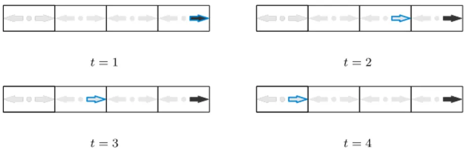
t = 1 t = 2
t = 3 t = 4
Fig. 3: The Lagrangian location (blue) of a distribution function given it’s Eulerian location (grey) in a 1D lattice as simulation time, t, advances.
A number of alternative data layout and streaming implementations exist to minimise or eliminate the need for duplication of data in the LBM. In this work, we use a technique called Lagrangian streaming[31]. As an LBM simu-lation proceeds, individual distribution functions stream in a single direction with a fixed step size. Viewed with an Eulerian reference frame, a distribution functions coordinates are constantly changing. However, if we view a distri-bution function with a Lagrangian reference frame, we can assign it a single location in memory. We then simply need a function to map a distribution functions Eulerian coordinates to Lagrangian coordinates, the relationship be-tween which is illustrated in figure 3. For a cubic domain this is given by
xl= (xe− teix)%Lx
yl= (ye− teiy)%Ly
zl= (ze− teiz)%Lz
(6)
where subscripts l and e denote coordinates in the Lagrangian and Eulerian frame respectively. L is the length of the domain, and % denotes the modulo operator.
2.3 Validation with Ideal Geometries
Two ideal porous geometries have been investigated to assess the performance of the partial bounceback boundary condition. These are periodic arrays of cylinders in 2D and spheres in 3D, arranged in a body-centered cubic configu-ration. Shown in figure 4, these geometries are deemed ideal as their definition is exact, and their permeability is well studied.
d L (a) (b) L d (c) (d)
Fig. 4: Validation geometry, (a,b) 2D case with cylinders, (c,d) 3D case with spheres
The lattice Boltzmann method has been validated for permeability ap-proximation of such geometries by a number of authors. In 2001 Hill et. al presented a study of arrays of packed spheres [32, 33]. Using Ladds half-way bounceback boundary condition [34] they compared simulation results to var-ious expressions for permeability, including those of Ergun and Carman which are to be discussed subsequently. The investigation of Hill et. al found that their LBM simulations offered a greater insight into the mechanisms governing permeability in such geometries. Further validation using this methodology in the Stokes flow regime was carried out by Van der Hoef et. al, who found their results to be within 3% of those already reported in the literature [35].
Based on these previous works, the lattice Boltzmann method with alter-nate boundary conditions is well validated for flow through sphere arrays. For the immersed boundary condition used in this work, validation was carried out in the Stokes flow regime by Leonardi et. al [36] where the model is reported to be accurate when compared with the results of Zick & Homsy [37]. In this sec-tion we extend this validasec-tion to include flows at moderate Reynold’s number. We begin first with a discussion of semi-empirical expressions used to predict the permeability of both cylinder and sphere arrays.
The problem of flow through pack columns has been extensively explored in published literature for at least 100 years. The first popular study of such flows was carried out by Kozeny [38], who’s work was subsequently extended upon by Carman [39]. The result of these studies was the well known Carman-Kozeny equation, which describes the Darcy permeability of a porous media under the Stokes flow regime. Later, Ergun the Darcy-Forcheimer permeability
of sphere packed beds by experimentation with a number of materials, arriving at Ergun’s equation [40]. d2 k + F Red= C1 (1− ϕ)2 ϕ3 + C2 (1− ϕ) ϕ3 Red (7)
where the expression has been normalised by sphere diameter. 150 and 1.75 have been used as values of C1 and C2 respectively [41].
By extending the Ergun’s equation, Liu et. al developed a new semi-empirical expression for Darcy-Forcheimer permeability [42]. The motivation for this new expression was to unify the work of Ergun and Carman-Kozeny. The result, is an expression which scales with ϕ−11/3(1− ϕ)2 as opposed to ϕ−3(1− ϕ)2 as in the orginal Carman-Kozeny expression. Later, Jeong et. al applied the lattice Boltzmann method to simulate the flow of fluid through a representative unit cell of packed spheres [43]. In their work, Jeong et. al noted that agreement with Ergun’s expression was limited to the case where porosity is low and the spheres are either contacting, or almost contacting. Since the sphere packing’s in Ergun’s experiments had consolidated under the action of gravity, this make sense. As a result, Jeong et. al propose the follow-ing expression, representfollow-ing a curve fit to their data which follows the form of the equation of Liu et. al.
d2 k + F Red= (162.4 + 3.0Red) [ ϕ11/3 (1− phi)2 ]−0.709 (8) Jeong et. al calibrated this expression using lattice Boltzmann models with a resolution of 60×60×60 lattice sites. To represent the solid boundaries they used the half-way bounceback condition [34], as opposed to an interpolated bounceback as is used in this work.
Whilst these equations are a good approximation for permeability of sphere packed columns, they are not directly applicable to the periodic cylinder ar-rays shown in figure 4. To investigate such a configuration Lee & Yang [41] constructed a numerical unit cell model of a periodic geometry consisting of cylinders of diameter, d. To approximate permeability they solved, implicitly, the equations of momentum and continuity. Their tests were carried out for a range of grain Reynolds numbers (0 < Red < 50). Results were summarised
by a curve fit which corresponds to their data within an average difference of 5%. kF = d2ϕ3(ϕ− 0.2146) 31(1− ϕ)1.3 F = (1− ϕ) 1.4 ϕ3(ϕ− 0.2146) 3 ∑ n=1 3 ∑ m=1 amnϕm−1Rend−1 [amn] = −17.754 0.5893 −0.0061604.825 −0.1660 0.00177 15.911 −0.4736 0.004836 (9)
where Lee & Yang used the form of Ergun’s expression as a basis for their own approximation.
The lattice Boltzmann models which have been constructed are based upon the methodology used by Lee & Yang. For both the 2D and 3D cases, a unit cell geometry was used and these are shown in figure 4. Flow through these geome-tries is modelled, and the results are used to approximate permeability within a range of Reynold’s numbers (0 < Red < 50) and porosities (0.43≤ ϕ ≤ 0.93).
Periodic cylinders
Variation of permeability with Reynold’s number for a packed column of cylin-ders is shown in figure 5. These models were run at a resolution of 250× 250 lattice sites, with a constant relaxation time of τ = 1.0. Solution proceeded until models achieved a steady state, when the change in total system energy between timesteps is sufficiently small. The average difference in permeability computed using the LBM and equation (9) is approximately 9.6%. However, if we restrict this comparison to porosities less than 0.74, then the average difference is approximately 5.7%. Since Lee & Yang’s expression matches their own results to within 5%, we can conclude that the accuracy of the LBM is on a par with the more traditional implicit solution carried out by Lee & Yang.
Red d 2 /K 0 10 20 30 40 50 100 101 102 103 φ = 0.43 φ = 0.50 φ = 0.60 φ = 0.74 φ = 0.85 φ = 0.93
Fig. 5: Permeability results for a periodic array of cylinders. ( ) Lee & Yang’s expression, ( ) LBM results.
Periodic spheres
Permeability tests were carried out for a periodic array of spheres under similar conditions as those for the periodic array of spheres. Due to computational limitations the model resolution in this instance was 100×100×100 lattice sites, with a fixed relaxation time of τ = 1.0. Variation of computed permeability with Reynold’s number is shown in figure 6, where expression (8) is also plotted for comparison. Red d 2 /K 0 10 20 30 40 50 100 101 102 103 φ = 0.43 φ = 0.50 φ = 0.60 φ = 0.74 φ = 0.85 φ = 0.93
Fig. 6: Permeability results for a periodic array of spheres. ( ) Expression of Jeong et. al, ( ) LBM results.
Within the limit of low Reynold’s number, our results are in better agree-ment with expression (8). Best agreeagree-ment with expression (8) is achieved in the lower porosity cases. Our results begin to diverge from the expression as Reynold’s number increases. This discrepancy could be potentially due to the difference in porosities explored in our analysis and that of Jeong et. al, where their expression appears to be calibrated against results for porosities of 0.3952 for the case of hexagonally packed spheres. In addition to this we expect the lower lattice resolution, and choice of boundary condition, to further influence the agreement between results.
Impact of boundary condition
To demonstrate the benefit of an immersed boundary condition, as opposed to the bounceback boundary condition, an analysis was carried out using the periodic cylinder array model. In this analysis the Reynold’s number, relax-ation time, and porosity were kept constant, while the domain resolution was varied with a side length of 5-250 lattice sites. Permeability approximations computed using this model are compared with equation (9) in figure 7, where normalised permeability is plotted against the ratio of pore throat width, T, to grid spacing, ∆x. T/∆x d 2 /K 4 8 12 16 20 24 28 32 20 40 60 80 100 120 140
Lee & Yang Bounceback Partial Bounceback
Fig. 7: Variation of Results with Increasing Geometric Definition
Comparing the boundary conditions in this way shows that computed per-meability results begin to stabilise at pore throat widths of 5 and 12 lattice units for the partial bounceback and bounceback boundary conditions respec-tively. In the stabilisation region, for throat widths between 4 and 24 lattice units, the solution error is less than 5% with partial bounceback, and 15% with bounceback. Both sets of results converge to a solution with an error of less than 1%.
The greater variation in results exhibited by the bounceback boundary condition is clearly due to the discretisation of the cylindrical boundary. As the domain resolution is varied the effective radius of the cylinder varies in a step-wise fashion, in some cases this effective radius is larger than the desired radius,
and vice versa. In the case of the partial bounceback condition this problem is avoided, however the lattice sites intersected by the boundary become porous due to the partial application of the bounceback condition. This is desirable when the obstacle is sufficiently larger than the lattice spacing, as it is required to more accurately capture the intersection of the obstacle and lattice sites. But in the case that the obstacle consists of only a small number of lattice sites, the obstacle may become completely porous, yielding an artificially high permeability as seen in the figure.
In this work, we are seeking to apply the LBM to permeability analysis of porous rock microstructures. The microstructure of sandstone contains ge-ometric features with characteristic length approaching (and below) the size of individual CT image voxels. The scale of surface roughness for instance is typically a number of orders of magnitude smaller than that of the grain ra-dius. This is especially pertinent if the CT images are downscaled. This test therefore demonstrates that the partial bounceback condition may offer a sig-nificant improvement over the bounceback boundary condition in capturing these smaller scale geometric features, with the provision that pore throat width is typically greater than 5 lattice units.
2.4 Digital Rock Analysis
This analysis is carried out on a sample of Diemelstadt sandstone supplied by the School of Earth and Environment, Leeds University, UK. Diemelstadt sandstone has a typical porosity of 0.24, and average grain radius of 80µm [44]. The nominal permeability of similar sandstones is reported as approximately 1D, and is typically isotropic [3, 45, 46, 4]. From this sample a CT image with a resolution of 1000vx3 (where vx denotes a voxel unit) was obtained. This sample is shown in figure 8a, with each voxel a cube of width 2µm. It should be noted that the porosity and permeability of the samples is unlikely to match exactly the nominal porosity and permeability of Diemelstadt sandstone due to the heterogeneous nature of rock material.
The voxelised geometry obtained through CT imaging is defined by a se-ries of densities corresponding to each voxel. By plotting a histogram of these densities in figure 9a, we see that the image includes two peaks in voxel den-sity which define the void and solid space within the sample. Voxel densities throughout the sample are, in general, normally distributed about these peaks. However, by plotting the histogram on a log scale in figure 9b we can see a broad range of voxel densities which do not fall in to these normal distribu-tions. These anomalous voxel densities are likely to be artifacts produced by the imaging process, and may be due to metallic inclusions in the sample [47]. The spatial distribution of anomalous voxel densities is shown in figure 8b. With artifacts present it is not possible to simply use the voxel densities to scale the partial bounceback boundary condition, as doing so would result in a domain that includes almost no solid lattice sites. Additionally, since these artifacts are spread throughout the sample it is not possible to sample a smaller
(a) (b)
Fig. 8: Diemelstadt sandstone CT scan showing (a) grain geometry and (b) imaging artifacts
0 0.5 1 1.5 2
(a)
0 0.5 1 1.5 2
(b)
geometry from the domain which would not include them. We therefore begin the analysis by filtering the artifacts.
Referring to figure 10b, we have defined three characteristic voxel densities, Vv, I, and Vs, representing a void, intermediate, and solid density respectively.
To filter out the imaging artifacts we reassign the corresponding voxel densities to either Vvor Vs, depending on their magnitude. If the artifact density exceeds
Vsits density is replaced with that of Vs. Conversely, if the artifact density is
less than Vv its density is replaced with that of Vv.
0 0.5 1 1.5 2
(a)
Vv I V
s
(b)
Fig. 10: Voxel density histograms following filtering of artifacts, with a (a) log scale and (b) linear scale annotated with segmentation parameters
Segmentation
Following filtering of artifacts the voxels must be segmented into void, solid and boundary regions so that they may be mapped to an LBM domain. In the works of [1, 3, 4] binary segmentation is applied, so that voxel densities above I
are deemed solid, and those below I are deemed void. Since we intend to apply the partial bounceback boundary condition to represent grey areas between solid and void space, a new process of segmentation must be defined which yields a mapping between the voxel density and β in equation (5).
To do this we introduce an upper and lower threshold to the voxel densities, Tu and Tl respectively. We then specify that voxel densities below Tl map to
β = 0.0, and voxel densities above Tumap to β = 1.0. Voxel densities between
Tland Tu are normalized to this range.
To asses the impact on segmentation on permeability approximation a threshold scaling parameter, α, is used to scale the upper and lower segmen-tation thresholds between Vv and Vsso that
Tl = I− α(I − Vv)
Tu = I + α(I− Vs)
(10) With this approach, binary segmentation is achieved when α = 0. As α increases the grain surfaces become more diffuse.
Scaling
In this work we use a GPU computing platform with a limited amount of RAM (6GB). In order to consider the entire sample geometry the CT image must be rescaled to a coarser resolution. To rescale the image, voxel densities in the destination were computed as the average density of the source image voxels they contained. Where the scaling process is carried out after segmentation has been applied. While the segmentation approach described is required in order to make use of the partial bounceback boundary condition, scaling is only required when a domain must be computed on a platform with limited memory.
(a) (b)
The scaling process employed is illustrated in figure 11. The average den-sity of the destination voxel is computed by taking weighted averages of the overlapped source voxels. The weights in this case are taken simply as the normalised volume of source and destination voxel intersection.
250vx3 200vx3
150vx3 100vx3
Fig. 12: Rescaling of CT image, where the initial 250vx3 image is subsampled from the original unscaled image
The effect of rescaling on geometric definition is demonstrated visually in figure 12, where a 250vx3subsample from the original CT image was incremen-tally rescaled to a resulting 100vx3 image. In applying this scaling algorithm the overall porosity of the image is maintained, as shown in figure 13. Con-sidering the dependence of permeability on porosity, this feature is key if any consistent measurements are to be achieved through image scaling.
Use of the partial bounceback boundary condition is advantageous when the CT image must be scaled, since the scaled voxel densities may be used directly and the consistence in porosity is maintained. This is not the case where the bounceback boundary condition is used as the image would require segmentation after scaling is applied, altering the porosity of the scaled image when compared with the source.
Resolution (vx³) Po ro s ity 50 100 150 200 250 0.1 0.15 0.2 0.25 0.3
Fig. 13: Measured image porosity through rescaling
3 Results
Using the lattice Boltzmann method and the partial bounceback boundary condition, a number of models have been built to assess the impact of image segmentation and scaling.
Segmentation
Using a scaled 200vx3CT image (scaled from 1000vx3), the threshold scaling parameter was varied across the range of valid values (0 ≤ α ≤ 1.0) in increments of 0.05. The LBM models were executed with a relaxation time of τ = 1.0, where the Reynold’s number was fixed at Re = 0.01. The choice of Reynold’s number was made so as to ensure a Stokes flow regime.
Figure 14a shows the variation of computed permeability with threshold scaling parameter. Figure 14b shows the corresponding change in effective porosity, where only pores which conduct fluid are included in porosity com-putation. The results show that the change in permeability is qualitatively related to the change in effective porosity, however the permeability changes at a much greater rate. A turning point is observed when α exceeds 0.75, figure 15 shows that at this point the grains themselves become porous.
These results are significant as they show that inclusion of only a small grey region between the grains and void space can have a pronounced effect on permeability approximation. Choosing α = 0.1 for instance results in a per-meability change of approximately 10%, where the change in effective porosity is only 2%.
While the change in permeability varies with porosity, the two parameters are not varying in proportion with one another. Thus, there is some amount
α P e rm e a b il it y ( D ) 0 0.25 0.5 0.75 1 3 4 5 6 7 8 9 10 (a) α E ff e c ti v e P o ro s it y 0 0.25 0.5 0.75 1 0.2 0.22 0.24 (b)
Fig. 14: Variation of (a) permeability and (b) effective porosity with α
(a) (b)
Fig. 15: CT image slices following segmentation for: (a) α = 0.5, (b) α = 0.75, Red = Solid, Blue = Void
of the permeability increase which is not due to the porosity increase. Further analysis of the segmented CT images shows a potential cause.
In figure 16 a CT image slice is shown following application of segmentation for two different values of alpha, 0.0 and 0.5. A single contour level has been added to the images, with a threshold of 0.75, where for voxel densities below
(a) (b)
Fig. 16: Contoured CT image slices following segmentation for: (a) α = 0.0, (b) α = 0.5. Colours have been adjusted to provide contrast to contour lines indicating grain boundaries
this value an appreciable volume of fluid may be conducted. These contours follow the effective grain boundaries.
We can see in the figure that, in general, pore radius is maintained. More significant however, is the change in pore connectivity. For the case of α = 0.0 a number of pores are separated by only a very thin boundary, when alpha is increased, this boundary becomes conductive, increasing the pore connectivity. This effect is most noticeable in the upper right corner of the images, were a relatively large system of pores becomes connected as α increases.
To account for this, percolation theory must be considered. Percolation theory suggests that the permeability of a porous medium may be related to porosity using a power law relationship [48] in which
k(ϕ) = C (ϕ− ϕcr) µ
(11) where C and µ are constants unique to the porous medium. ϕcr is the critical
porosity, the porosity below which percolation may not theoretically occur. In percolation theory, the critical porosity is known as the percolation threshold. For a lattice of potentially connected voids the percolation threshold is in-versely proportional to the average number of connected neighbours [49] each void has, or coordination number, Z.
ϕcr∝
1
Z (12)
From these equations it is known that if the connectivity between pores increases, the percolation threshold decreases with a resultant increase in per-meability, as observed in these results. So if binary segmentation is applied, the pore connectivity of the image may be artificially reduced.
Whilst it is clear that the threshold scaling parameter should be set such that α < 0.75, it is not possible to determine an exact value from this analysis. A reasonable estimate would be possible if the sample were tested for perme-ability. However heterogeneity in the sample will lead to a range of measured permeabilities, so α could only be defined within a corresponding range. Ul-timately, the best way to find an exact value for α would be to test only the part of the sample that was imaged for modelling, and repeat the analysis we have carried out here to find a value of α which yields a model with correct permeability. While such a procedure would be possible, it was not feasible for this study.
In the absence of a more rigorous process for determination of α, visual analysis was used to select an appropriate value for the results which follow. This value was chosen as α = 0.5, where it is shown in figure 15 that this choice results in solid grains with a grey region at the grain/void boundary.
Image scaling
By taking a random series of 250vx3subsamples from the original CT image,
we looked at the effect a change in resolution through image scaling has on permeability approximation. 5 subsamples were scaled in increments of 50vx3
from 250vx3 to 50vx3, yielding a set of 25 model geometries. Using a lattice
Boltzmann model, permeability was approximated for a fixed Reynold’s num-ber and a relaxation time of τ = 1. In addition to approximating permeability effective porosity was also measured, as the investigation into segmentation showed results will be sensistive to any change in effective porosity.
Results for computed permeability and effective porosity are shown in fig-ure 17. In the figfig-ure, each curve shown represents results from a single original subsample. The general trend observed was one of increasing permeability as the image was coarsened, however the trend is not smooth. Permeability was observed to achieve a maximum for the 150vx3 models. It is expected that
this would correspond to a maximum in effective porosity, however at this resolution the effective porosity of the model geometry was typically at it’s lowest.
The general increase in permeability relative to the unscaled image is most likely attributed to lack of a reasonable number of lattice sites at the pore throats. In addition to this, as the image was coarsened the grain surfaces became smoother. The inconsistency in permeability variation also indicates that image scaling fails to maintain a consistent connectivity between pores. Finally, image scaling leads to a more diffuse grain boundary, further affecting the pore throat diameter.
Based on these results it is our recommendation that permeability assess-ment on such CT images be carried out at the highest feasible resolution, maintaining a sufficient number of lattice sites across the pore throats. The simple arithmetic averaging approach to image scaling used in this work lead to highly inconsistent behaviour, which appear to be essentially random.
Fu-Resolution (vx³) Effe c ti v e Po ro s ity 50 100 150 200 250 0.1 0.15 0.2 0.25 0.3 (a) Resolution (vx³) Pe rm e a b il ity (D ) 50 100 150 200 250 0 1 2 3 4 5 (b)
Fig. 17: Variation of (a) effective porosity and (b) permeability with scaling resolution, each curve represents a random sample fromt he original CT image.
ture attempts at coarsening CT images should focus not just on maintaining overall porosity, but also on surface roughness and pore connectivity.
Non-Darcy Permeability
Through the course of running these tests it became apparent that Reynold’s number can also be a significant factor affecting permeability approximation, even if Stokes flow is assumed. In figure 18 computed permeability is plotted against Reynolds number, for two values of alpha. To produce the results for the figure, Reynolds number was varied in the range 0.01 ≤ Re ≤ 0.25, corresponding to a maximum flow rate of 5× 10⁻⁴ m/s.
The observed increase in permeability across the range of Reynold’s num-bers tested was less extreme for the case of binary thresholding. It was however not insignificant, comparing the flow of Reynold’s number 0.25 with that of 0.01, an increase in permeability of approximately 32% is found.
A potential source of the observed permeability increase may lie in the weakly compressible assumption of the LBM. For the LBM to accurately re-produce Navier-Stokes flow, the Mach number must be sufficiently low to avoid compressibility effects. Where such effects would introduce strongly non-linear behaviour in the flow solution. In these tests however the Mach number never exceeded 8.3× 10⁻⁴.
Non-Darcy behaviour in porous rock models has been previously observed by both Sukop et. al and Yang et. al. Through modelling of vuggy limestone using the LBM with binary segmentation, Sukop et. al observed decreases in
Reh Pe rm e a b ili ty (D ) 0 0.1 0.2 4 5 6 7 8 9
Fig. 18: Comparison of permeability-Reynolds number relationship for α = 0.0 ( ) and α = 0.5 ( )
permeability for Reynold’s numbers above 0.01 [50]. Yang et. al numerically approximated the permeability of waste water flocs using FLUENT 6.0 (Flu-ent Inc., USA). Yang et. al found that, given a Reynold’s number greater than 1, permeability may increase, decrease, or remain constant [51]. Where the ex-act nature of permeability changes was dependent on differences in tortuosity between larger and smaller pore channels.
In this work, and those cited, the modelled flow rates are sufficiently low to ensure laminar flow. Though none of these works are in exact agreement on the nature of permeability changes, it is generally agreed that flow rate dependent permeability may be observed at Reynold’s numbers typically associated with a purely Darcy flow regime.
4 Conclusion
It has been shown by various authors that it is possible to compute accurate ap-proximations of permeability from CT images of porous rock microstructures using the LBM. However the choice of boundary condition and associated segmentation used in these studies may lead to an underestimation of pore connectivity when compared with the raw CT image data. We have proposed that instead of using the bounceback boundary condition, the IMB condition of Noble & Torczynski should be used as a partial bounceback boundary con-dition so that the grey regions of the CT image data may be considered in the model.
Validation of the partial bounceback boundary condition for permeabil-ity approximation was carried out by simulating flows through ideal porous geometries consisting of cylinders and spheres. Comparison with the work of
Lee & Yang and Jeong et. al shows that this boundary condition is able to accurately reproduce their permeability approximations, whilst outperforming the bounceback boundary condition where model resolution is low.
The partial bounceback boundary condition was then applied to simulate the flow of fluid through rock microstructures, obtained through CT imaging. We varied the mapping of CT image data to the solid volume fraction pa-rameter in the partial bounceback boundary condition. Particular attention was paid to image segmentation and scaling. It was shown that correct im-age segmentation is vital if accurate permeability results are to be obtained, our results suggest that binary segmentation can lead to underestimation of permeability and pore connectivity. Where image scaling was applied, perme-ability was not found to vary consistently with changes in model resolution. To resolve this, a scaling technique which maintains the effective porosity and pore connectivity should be devised. Whilst the partial bounceback condition shows promise in the ability to apply a more flexible approach to segmenta-tion, the image scaling investigated in this work is not recommended if absolute accuracy is to be achieved.
Ultimately, this investigation shows that small changes in boundary defi-nition may have a significant impact on the computed permeabilities, where the change in effective porosity may still be small.
References
1. Edo S Boek and Maddalena Venturoli. Lattice-Boltzmann studies of fluid flow in porous media with realistic rock geometries. Computers & Mathematics with Applications, 59(7):2305–2314, 2010.
2. Benjamin Ahrenholz, Jonas T¨olke, and Manfred Krafczyk. Lattice-Boltzmann simula-tions in reconstructed parametrized porous media. International Journal of
Computa-tional Fluid Dynamics, 20(6):369–377, July 2006.
3. N Lenoir, JE Andrade, WC Sun, and JW Rudnicki. In situ permeability measurements inside compaction bands using X-ray CT and lattice Boltzmann calculations. Proc.
GeoX, 2010.
4. Avrami Grader, Yaoming Mu, Jonas Toelke, and Chuck Baldwin. Estimation of relative permeability using the Lattice Boltzmann method for fluid flows, Thamama Formation, Abu Dhabi. In Proceedings of the Abu Dhabi International Petroleum Exhibition &
Conferences, Abu Dhabi, 2010.
5. Irina Ginzburg and Dominique DHumi`eres. Multi-reflection boundary conditions for lattice Boltzmann models. Physical Review E, 68(6):066614, 2003.
6. D. R. Noble and J. R. Torczynski. A Lattice-Boltzmann Method for Partially Saturated Computational Cells. International Journal of Modern Physics C, 09(08):1189–1201, December 1998.
7. Cyrus K. Aidun and Jonathan R. Clausen. Lattice-Boltzmann Method for Complex Flows. Annual Review of Fluid Mechanics, 42(1):439–472, 2010.
8. Aydin Nabovati, Edward W Llewellin, and Antonio C M Sousa. A general model for the permeability of fibrous porous media based on fluid flow simulations using the lattice Boltzmann method. Composites Part A: Applied Science and Manufacturing, 40(6-7):860–869, 2009.
9. Zhaoli Guo and T. Zhao. Lattice Boltzmann model for incompressible flows through porous media. Physical Review E, 66(3):036304, September 2002.
10. Rita G. Lerner and George L. Trigg. Encyclopedia of Physics. Wiley, 2nd edition, 1990. 11. I. G. Currie. Fundamental Mechanics of Fluids. Marcel Dekker, Inc., 3rd edition, 2003.
12. S. Chapman and T. G. Cowling. The Mathematical Theory of Non-uniform Gases. An Account of the Kinetic Theory of Viscosity, Thermal Conduction and Diffusion in Gases. Cambridge University Press, 1991.
13. Shiyi Chen and Gary D. Doolen. Lattice Boltzmann Method for Fluid Flows. Annual
Review of Fluid Mechanics, 30(1):329–364, 1998.
14. Dieter A Wolf-gladrow. Lattice-Gas Cellular Automata and Lattice Boltzmann Models
- An Introduction. Springer, 2005.
15. Daniel H. Rothman. Cellular-automaton fluids: A model for flow in porous media.
Geophysics, 53(4):509, 1988.
16. Guy R. McNamara and Gianluigi Zanetti. Use of the boltzmann equation to simulate lattice-gas automata. Physical Review Letters, 61(20):2332–2335, 1988.
17. F. J Higuera and J Jim´enez. Boltzmann Approach to Lattice Gas Simulations.
Euro-physics Letters (EPL), 9(7):663–668, 2007.
18. P. L. Bhatnagar, E. P. Gross, and M. Krook. A model for collision processes in gases. i. small amplitude processes in charged and neutral one-component systems. Phys. Rev., 94:511–525, May 1954.
19. Y H Qian, D D’Humi`eres, and P Lallemand. Lattice BGK Models for Navier-Stokes Equation. EPL (Europhysics Letters), 17:479, 1992.
20. Hudong Chen, Shiyi Chen, and William H. Matthaeus. Recovery of the Navier-Stokes equations using a lattice-gas Boltzmann method. Physical Review A, 45(8):R5339–
R5342, April 1992.
21. Y T Feng, K Han, and D R J Owen. Coupled lattice Boltzmann method and discrete element modelling of particle transport in turbulent fluid flows: Computational issues.
International Journal for Numerical Methods in Engineering, 72(9):1111–1134, 2007.
22. D’Humieres. Generalized lattice-Boltzmann equation. In Rarefied Gas Dynamics:
The-ory and Simulations, pages 440–458. ICASE, 1992.
23. Chongxun Pan, Li-Shi Luo, and Cass T. Miller. An evaluation of lattice Boltzmann schemes for porous medium flow simulation. Computers & Fluids, 35(8-9):898–909, September 2006.
24. Dominique D’Humi`eres and Irina Ginzburg. Viscosity independent numerical errors for Lattice Boltzmann models: From recurrence equations to ”magic” collision numbers.
Computers and Mathematics with Applications, 58(5):823–840, 2009.
25. Xiaoyi He, Qisu Zou, Li-Shi Luo, and Micah Dembo. Analytic solutions of simple flows and analysis of nonslip boundary conditions for the lattice Boltzmann BGK model.
Journal of Statistical Physics, 87(1):115–136, 1997.
26. Christopher Ross Leonardi. Development of a Computational Framework Coupling the Non-Newtonian Lattice Boltzmann Method and the Discrete Element Method with Application to Block Caving. PhD thesis, Swansea University, 2009.
27. D. J. Holdych. Lattice Boltzmann methods for diffuse and mobile interfaces. PhD thesis, University of Illinois at Urbana-Champaign, 2003.
28. O Erik Strack and Benjamin K Cook. Three-dimensional immersed boundary conditions for moving solids in the lattice-Boltzmann method. International Journal for Numerical
Methods in Fluids, 55(2):103–125, 2007.
29. Yu Ye, Peng Chi, and Yan Wang. An efficient implementation of entropic lattice boltz-mann method in a hybrid cpu-gpu computing environment. In Kenli Li, Zheng Xiao, Yan Wang, Jiayi Du, and Keqin Li, editors, Parallel Computational Fluid Dynamics, volume 405 of Communications in Computer and Information Science, pages 136–148. Springer Berlin Heidelberg, 2014.
30. P. Bailey, J. Myre, S.D.C. Walsh, D.J. Lilja, and M.O. Saar. Accelerating lattice boltz-mann fluid flow simulations using graphics processors. In Parallel Processing, 2009.
ICPP ’09. International Conference on, pages 550–557, Sept 2009.
31. F. Massaioli and G. Amati. Achieving high performance in a LBM code using OpenMP. In The Fourth European Workshop on OpenMP, Roma, Italy, 2002.
32. Reghan J. Hill, Donald L. Koch, and Anthony J. C. Ladd. The first effects of fluid inertia on flows in ordered and random arrays of spheres. Journal of Fluid Mechanics, 448:213–241, November 2001.
33. Reghan J. Hill, Donald L. Koch, and Anthony J C Ladd. Moderate-Reynolds-number flows in ordered and random arrays of spheres. Journal of Fluid Mechanics, 448:243– 278, 2001.
34. AJC Ladd. Numerical simulations of particulate suspensions via a discretized Boltz-mann equation. Part 2. Numerical results. Journal of Fluid Mechanics, 271:285–309, 1994.
35. M. a. Van Der Hoef, R. Beetstra, and J. a. M. Kuipers. Lattice-Boltzmann simulations of low-Reynolds-number flow past mono- and bidisperse arrays of spheres: results for the permeability and drag force. Journal of Fluid Mechanics, 528:233–254, 2005. 36. Christopher R Leonardi, Bruce D Jones, David W Holmes, and John R Williams.
Simu-lation of complex particle suspensions using coupled lattice Boltzmann-discreet element methods. In 6th International Conference on Discrete Element Methods (DEM6), 2013. 37. G M Homsy. Stokes flow through periodic arrays of spheres. Journal of fluid mechanics,
115:13–26, 1982.
38. J. Kozeny. ¨Uber kapillare Leitung des Wassers im Boden. Akad. Wiss. Wien, 136:271– 306, 1927.
39. P. C. Carman. Fluid flow through granular beds. Chemical Engineering Research &
Design, 75:S32 – S48, 1937.
40. Sabri Ergun and a. a. Orning. Fluid Flow through Randomly Packed Columns and Fluidized Beds. Industrial & Engineering Chemistry, 41(6):1179–1184, June 1949. 41. S L Lee and J H Yang. Modeling of Darcy-Forchheimer drag for fluid flow across a bank
of circular cylinders. International Journal of Heat and Mass Transfer, 40(13):3149– 3155, 1997.
42. Shijie Liu, Artin Afacan, and Jacob H Masliyah. Steady Incompresible Laminar Flow in Porous Media. Chemical Engineering Science, 49(21):3565–3586, 1994.
43. Namgyun Jeong, Do Hyung Choi, and Ching-Long Lin. Prediction of DarcyForch-heimer drag for micro-porous structures of complex geometry using the lattice Boltz-mann method. Journal of Micromechanics and Microengineering, 16(10):2240–2250, October 2006.
44. Laurent Louis, Teng-fong Wong, Patrick Baud, and Sheryl Tembe. Imaging strain localization by X-ray computed tomography: discrete compaction bands in Diemelstadt sandstone. Journal of Structural Geology, 28(5):762–775, May 2006.
45. J Guodong, TW Patzek, and D Silin. Direct prediction of the absolute permeability of unconsolidated and consolidated reservoir rock. In SPE Annual Technical Conference
and Exhibition, Houston, Texas, 2004.
46. Hiroshi Okabe. Pore-Scale Modelling of Carbonates. PhD thesis, Imperial College London, 2004.
47. F. E. Boas and D. Fleischmann. CT artifacts: causes and reduction techniques. Future
Medicine, 4(2):229–240, 2012.
48. K. Maruyama, O. Koichi, and S. Miyazima. Critical exponents of continuum percolation.
Physica A, 191:313–315, 1992.
49. A. Hunt, R. Ewing, and B. Ghanbarian. Percolation Theory for Flow in Porous Media. Springer International Publishing, 1 edition, 2014.
50. Michael C. Sukop, Haibo Huang, Pedro F. Alvarez, Evan a. Variano, and Kevin J. Cunningham. Evaluation of permeability and non-Darcy flow in vuggy macroporous limestone aquifer samples with lattice Boltzmann methods. Water Resources Research, 49(1):216–230, January 2013.
51. Zeng Yang, Xiao-Feng Peng, Duu-Jong Lee, and Ay Su. Reynolds number-dependent permeability of wastewater sludge flocs. Journal of the Chinese Institute of Chemical