Edge and Region Segmentation Based Video
Coding Method
by
Kuniaki Takahashi
Submitted to the Department of Electrical Engineering and
Computer Science
in partial fulfillment of the requirements for the degrees of
Master of Engineering
and
Bachelor of Science in Electrical Engineering
at the
MASSACHUSETTS INSTITUTE OF TECHNOLOGY
February 1998
@Massachusetts Institute of Technology 1998. All rights reserved.
Author...
...
Department of Elect; aEngineering and Computer Science
Feb 4, 1998
Certified by...
...
Berthold K. P. Horn
Professor
jheis
upervisor
Accepted by ... ...
..
...
....
Arthur C. Smith
Chairman, Department Committee on Graduate Students
Edge and Region Segmentation Based Video Coding
Method
by
Kuniaki Takahashi
Submitted to the Department of Electrical Engineering and Computer Science on Feb 4, 1998, in partial fulfillment of the
requirements for the degrees of Master of Engineering
and
Bachelor of Science in Electrical Engineering
Abstract
This thesis examines an edge detection and region segmentation based image compres-sion scheme for applications in very low bit rate video coding. At high comprescompres-sion rates, edge detection based image coding results in line artifacts protruding from breaks in contours caused by smearing of the foreground and background. We pro-pose an algorithm that combines edge detection and region segmentation to improve the image quality for a fixed compression rate. We describe the development of the region segmentation based algorithm, and compare the image quality with the edge based compression method.
Thesis Supervisor: Berthold K. P. Horn Title: Professor
Acknowledgments
First of all, I would like to thank Dr. Ichiro Masaki, for his guidance, constant
support, patience, wisdom and understanding. Thank you for bearing with me, and
teaching me many things about research and life. It was a great privilege working
with him.
I would like to thank my research supervisor Prof. Berthold Horn for his fine
advice and great intelligence. I am grateful to him for providing helpful suggestions.
Many thanks to Marcelo Mizuki who always willingly helped me with my questions
and directed me to the right resources. Thanks to Paul, Robbin, Haiqian, Nicole,
Yajun, and all other members of the AI Lab for their support.
Finally, I would like to thank my family back in Japan for all their love, and for
supporting my decision to leave the country to study at MIT.
Contents
1 Introduction
1.1 Thesis organization ...2 Background
2.1
Image compression
...
2.2 Region segmentation ...2.3 Compression schemes for low-bit rate video coding . ...
3 Region Segmentation of One-Dimensional Spatial Intensity
3.1 Proposed method . ... 3.2 Mean based approach ...
3.2.1 Region Merging ... 3.2.2 Region Division ... 3.2.3 Problems with Mean-based 3.3 Line fitting Approach ...
3.3.1 Motivation ... 3.3.2 Region merging ... 3.3.3 Region Division ... 3.3.4 Thinning of thick edges . 3.4 Continuity Issues . ...
3.4.1 Breaks in contours . . 3.4.2 Modifications in the thinnii 3.4.3 Problems with Contour Fil
region segmentation
g operation ... terin ...
3.4.4
Region width ...
...
. .
...
.
43
3.5 Intensity coding ...
.
...
...
43
3.6 Encoder Block Diagram .
...
...
...
44
4 Performance Results
47
4.1 Performance and Results ...
...
47
4.2
Results
...
...
47
4.2.1
Region segmentation without Sobel and Level edge detection .
47
4.2.2
Hybrid method of Sobel and Region Segmentation ...
48
4.3
Conclusion ...
...
..
53
4.4
Suggestions for future work
...
....
56
List of Figures
3-1 Illustration of Region Definition ... .. 19 3-2 Region Segmentation Process . . ... ... .. . 20 3-3 Diagram illustrating Mean Based merging parameters . ... 24 3-4 1-D illustration of Mean-based merging process. (a) Examined region
has A3 _ Mthreshold. (b) The edge dividing the two regions is removed. (c) The next step examines the combined region and the next adjacent
region ... ... ... .. 25
3-5 Merging process when threshold is exceeded. (a) Examined region has
A3 > Mthreshold. (b) The next step examines the regions as illustrated. 26 3-6 Illustration of Region Division parameters . ... 28 3-7 1-D illustration of Region Division operation. (a) Examined region has
A3 > Dthreshold.
(b)
Region is temporarily divided into two smaller regions by a virtual edge. Leftmost region is examined and A3 >Dthreshold. (c) Leftmost region is separated and virtual edge is placed.
Previous virtual edge is ignored. Leftmost region is examined again
where A3 < Dthreshold. ... . . .. ... .. 29 3-8 Virtual edge is replaced with real edge and next adjacent region is
examined. ... ... ... 30
3-9 Illustration of why Ramp-like behavior of intensity will cause placement of region boundary in slow transition zone. (a) The intensity is slowly varying and A > Dthreshold. (b) A false edge is placed in the region
division process. . ... . . ... .. 32 3-10 Illustration of line-fitted region merging process . ... 34
3-11 Illustration of thinning of successive edges. (a) Edges placed in suc-cession. (b) Thin by removing all edges in between end-edges. The resulting regions produce a better fitted line. (c) Thin by removing all edges except midpoint edge. The remaining edge is half that of the method (b), however the fitted lines have a larger error. . ... 37
3-12 Illustration of pels used in weighted intensity calculation ... 39
3-13 Pels used in thinning method. c, u, d, 1 and r represent the gradients at the current, up, down, left and right pixels, respectively. ... . 40 3-14 Branching causing different results after contour filtering (a) Edge is
added through region division that results as a branch from the origi-nal contour. (b)The contour is counted by the contour filtering algo-rithm as two shorter contours. (c) The shorter contour is now removed through the filtering process . ... ... .... 42
3-15 Problems with curved contours with peaks towards the top of the image 43
3-16 Block Diagram of Color Static Encoder using Region Segmentation . 45 4-1 (a)Binary edge map with low Sobel threshold of "Lenna" at 0.275
bpp.(b)Binary edge map using hybrid method at 0.270 bpp. ... 48
4-2 (a)Interpolated image (without mean coding) of "Lenna" using orig-inal algorithm at 0.275 bpp. (b) Interpolated image (without mean coding) of "Lenna" using proposed algorithm at 0.270 bpp. There is less smearing of the image especially around the pillar to the left of the
image. ... ... ... 49
4-3 (a)Reconstructed image (with mean coding) of "Lenna" using original algorithm at 0.275 bpp. (b) Reconstructed image (with mean coding) of "Lenna" using proposed algorithm at 0.270 bpp. The definition of the pillar to the left of the image is improved. . ... . 49
4-4
(a) Enlarged section of the contour mapping the brim of the hat in
the original binary edge map for "Girl2" image. (b) Region Division
adds two edges along the contour. The locations is signaled by the
grey arrow. The contour filtering algorithm splits the contour into
the portion to the right of the added edges and the remaining portion
to the left is split into contours of 2 to 3 pixel lengths. The contour
filtering process then removes all the portion of the contour to the left
of the added edges with a minimum contour length of 7. . ...
52
4-5
Original color images displayed in monochrome (a) Girl2 (b) Cablecar
(c) Sailboat ...
...
53
4-6 Binary Edge maps obtained from Sobel and Level Edge Detection (a)
Girl2 (b) Cablecar (c) Sailboat ...
...
. . .
53
4-7 Binary Edge maps obtained from Sobel and Level Edge Detection and
Region Division (a) Girl2 (b) Cablecar (c) Sailboat . ...
54
4-8 Binary Edge maps obtained from Sobel and Level Edge Detection,
Region Division and Region Merging (a) Girl2 (b) Cablecar (c) Sailboat 54
4-9 Interpolated color images (without mean coding) from Sobel and Level
Edge Detection displayed in monochrome (a) Girl2 (b) Cablecar (c)
Sailboat ...
...
54
4-10 Interpolated color images (without mean coding) with Region
Segmen-tation displayed in monochrome (a) Girl2 (b) Cablecar (c) Sailboat
55
4-11 Reconstructed color images (with mean coding) from Sobel and Level
Edge Detection displayed in monochrome (a) Girl2 (b) Cablecar (c)
Sailboat ...
..
...
55
4-12 Reconstructed color images (with mean coding) with Region
Segmen-tation displayed in monochrome (a) Girl2 (b) Cablecar (c) Sailboat
.
55
List of Tables
4.1 PSNR comparison for original and Region Segmentation method for
the "Lenna" image. The results for the original method have "N/A" in
the Region Division Threshold (Dthreshold) and Region MergingThresh-old
(Mthreshold).PSNR 1 is without mean coding and PSNR 2 is with
mean coding ...
...
...
50
4.2 PSNR comparison for original and Region Segmentation method for
the "Sailboat" image. PSNR 1 is without mean coding and PSNR 2 is
with mean coding ...
...
51
4.3 PSNR comparison for original and Region Segmentation method for
the "Girl2" image. PSNR 1 is without mean coding and PSNR 2 is
with mean coding ...
.
...
51
4.4 PSNR comparison for original and Region Segmentation method for
the "Cablecar" image. PSNR 1 is without mean coding and PSNR 2
Chapter 1
Introduction
The increase in use of video conferencing over mobile telephone networks or the Pub-lic Switched Telephone Network (PSTN) has produced a high demand for image compression techniques that can transmit data at very low bit-rates. Various indus-try standards for video and image compression, such as the Joint Photographic Ex-perts Group (JPEG) still frame coding standard, the Motion Picture ExEx-perts Group (ISO-IEC MPEG) video coding standard [1], and the ITU-T H.261 video telephony standard have been established. However, these standards fail to provide substantial image quality for very high compression rates. To meet the bandwidth limits1 of the Public Switched Telephone Network (PSTN) using an analog phone line, or Radio Frequency (RF) used in mobile telephone networks, a compression ratio on the order of 100:1 or higher is required. At such high compression ratios, the block-based trans-form coding techniques used in JPEG, MPEG and H.261 break down, and significant block effects that distort the image become apparent. For such low bit-rate applica-tions, other approaches for coding at high compression ratios need to be developed to satisfy the requirements for video telephony.
This thesis examines a video image compression algorithm for image data for very low bit rate applications. The coding scheme is based on a hybrid of edge detection and region segmentation. The video image compression is subdivided into
two essential parts, the static image coding and the interframe coding. The static coding reduces the spatial redundancy in the image, and the interframe coding reduces the temporal redundancy between image frames. The development of the system is based on previous work done by Desai, Mizuki, Masaki and Horn [2] on edge and mean based image compression. Modifications are made to the compression algorithm, to enhance the image quality while maintaining or further increasing the high compression ratio of over 100:1. The proposed approach uses a hybrid edge detection and region segmentation [3] method for static image coding.
1.1
Thesis organization
Chapter 2 discusses various image compression and region segmentation techniques. Chapter 3 describes the development of the algorithm for region segmentation. Var-ious approaches for region segmentation are examined, together with the issues in-volved in integrating the algorithm with the encoder and decoder developed in [2]. Chapter 4 describes the performance of the proposed algorithm, and suggestions for further work.
Chapter 2
Background
This chapter discusses the various techniques for coding static images. The methods described here provide background for understanding the diversity in coding algo-rithms that span from conventional to aggressive. A discussion of the position of our proposed coding algorithm within the spectrum of various compression techniques is described. Various approaches for region segmentation are also discussed.
2.1
Image compression
Aggressive image compression methods have been studied to obtain very low bit-rates. Methods using models that learn, track and recognize behavior have been developed and implemented using state-based approaches [4] [5] [6]. Hidden Markov Models (HMMs) have also been a popular technique for recognizing gestures [7]. Another model based method involves using the finite element method to model elements of the human face such as lips [8]. When applied in laboratory environments where the models are trained specifically for the task, the model based methods perform well in recognizing gestures, resulting in a significant reduction in transmitted data. However, the model based methods are limited to strictly controlled environments, and have not yet reached the state to which they can perform in natural environments. Other difficulties such as having to mark points on the face to function as cues to detect movement [8], also limit the practicability of the aggressive methods at present.
Conventional image compression methods have been developed for a wide range of applications such as media storage or meeting bandwidth requirements. Detailed description of image coding fundamentals can be found in [9]. The conventional methods described as waveform coding techniques are grouped into the following classifications:
* Pulse Code Modulation (PCM)
* Predictive
* Transform/Subband
* Interpolative and Extrapolative * Statistical Coding
* Other methods
In PCM, each pixel is processed independently, ignoring the inter pixel dependen-cies. The amplitude and time are sampled and quantized using 2k levels. In predictive coding, the approach is to remove mutual redundancy between successive pixels and encode only the new information. In transform coding, the image data is linearly transformed into a different domain, where the coefficients are quantized and selected for transmission. Cosine transforms have become more popular in recent years be-cause they appear to be well matched to the statistics of the image data. In subband coding, the image waveform is decomposed into several subband pictures through a bank of bandpass filters. Each subband picture is then subsampled and coded. In-terpolative and Extrapolative coding works on a different principal. They attempt to transmit a subset of the pels to the receiver, and then interpolate or extrapolate the untransmitted pels. Statistical coding minimizes the average bit rate by assigning bits based on long-term average statistics or short-term statistics of the data. Other methods include vector quantization, contour coding and run-length coding [10] [11]. A practical coding system will often use a combination of the above compression methods.
2.2
Region segmentation
In this thesis, we propose an image compression method using image segmentation techniques. A detailed description of several generic methods of image segmentation can be found in [12] [3]. There is no theory of image segmentation. Segmentation entails the division or separation of an image into regions of similar attributes. Unfor-tunately, no quantitative image segmentation performance metric has been developed. Studies have been done to segment regions by dilation and erosion of neighboring pixels [13] [14] [15]. In these methods, the dilation and erosion operations are re-cursively implemented until every pixel within the image belongs to a region. Ahuja [16] introduces a transform for multi-scale image segmentation. However, the two dimensional computation using multiple scales is expensive and is not practical for real time segmentation. Other methods segment images in conjunction with edge detection [17] [18] [19]. Most region segmentation techniques involve extensive calcu-lations to determine the homogeneity of the pels within a region. A simpler approach needs to be developed to allow for region segmentation in real time.
2.3
Compression schemes for low-bit rate video
coding
With conventional transform based static image compression methods such as JPEG, very high compression results in unpleasant block distortion in the reconstructed image. In recent years, demand for video coding at a very low bit-rate has increased, and has been studied for mobile visual communication, on which a very narrow band width is used.
To solve the distortion problems related to low-bit rate video coding in standard coding methods, Yokoyama, Miyamoto and Ohta [20] proposed a method using mo-tion compensamo-tion based on arbitrarily shaped regions. This method uses a region growing method [14] to segment the image into arbitrarily shaped regions. In this method, a bit-rate of 9.6kb/s is achieved for a 176x144 color image at 7.5 frames/s,
where every fourth original frame is coded. However, compression methods with higher data reduction are desired to allow for images of higher resolution.
Desai et al. [2] proposed a method which relies on edge data to achieve a high compression ratio with better subjective image quality than standard compression methods employed in ITU-T H.261 or ISO-IEC MPEG. However, the edge detec-tion method implemented in Desai et al., has shortcomings. In order to achieve the high compression rate of 100:1, a high threshold is used on the Sobel and Level edge detectioni which lead to breaks in contours. This causes unpleasant line artifacts by smearing together the intensity of the foreground and background when reconstruct-ing the image. The operator used for edge detection is also susceptible to noise due to the limited 3 x 3 local intensity data incorporated in each gradient calculation. This results in detection of noise-induced edges.
Modifications can be made in this edge based compression scheme to enhance the image quality and reduce it's susceptibility to noise. A proposed modification is to use region segmentation. We propose to use a region segmentation method specifically designed to utilize the edge information produced from Sobel and Level edge gradient calculations. The region segmentation operation should produce regions with bound-aries that optimize the intensity reconstruction using linear interpolation. Therefore, to be consistent with the one-dimensional linear interpolation reconstruction process, and for computational efficiency, a one-dimensional region segmentation method is proposed.
1
Sobel and Level edge gradients are obtained by combining the results of convolving the input image with filters that calculate the horizontal and vertical differentiation. Edges obtained using the Sobel detector are usually sharp. Level edges are used in conjunction with Sobel edge detection to detect slowly-varying edges.
Chapter 3
Region Segmentation of
One-Dimensional Spatial Intensity
In this thesis, a method for enhancing the image quality of the edge and mean based
image compression method is proposed. The proposed compression algorithm uses a
hybrid of edge detection [2] and region segmentation. Region segmentation is used to
incorporate more global intensity information for determining the criteria for adding
or removing edges. In this proposed method, edges are defined as region boundaries
along horizontal and vertical scan lines.
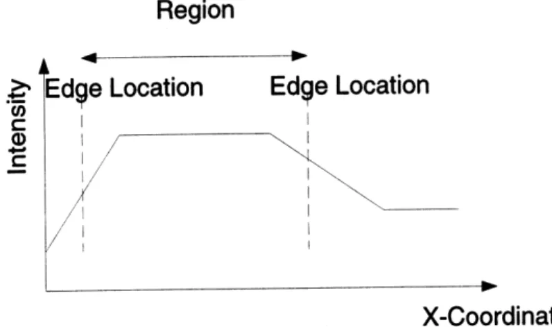
Region
Co C
Q) C
Edge
Location
Edge Location
X-Coordinate
Figure 3-1: Illustration of Region Definition
The intensity information within a region is used to compute a measure to compare
with a pre-defined threshold. Various measures such as deviation from the mean
intensity value or the deviation from an intensity line fitted value will be explored in this chapter to compare against the pre-defined threshold.
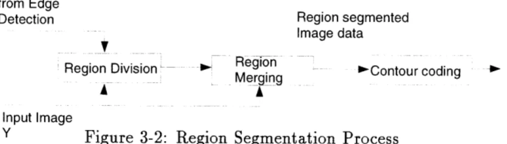
The measure is compared with the threshold as a criterion to determine the loca-tion of region boundaries. Incorporating more global data in comparison to the local-ized 3x3 Sobel operator used in Desai et al., when computing the measure reduces the possibility of noise-induced edges resulting from placement of region boundaries. Figure 3-2 shows a block diagram of the region segmentation process.
Divided regions from Edge
Detection Region segmented Image data
Region Division R ion Merging " Contour coding
A A
Input Image
Y Figure 3-2: Region Segmentation Process
For region division, the computed measure is compared with the threshold as a criterion to determine if the region needs to be split into smaller regions. An edge is placed at the region boundary where the algorithm decides to divide the region. Possible locations for the region boundary such as the point of maximum deviation of the line fitted value to the original intensity value will be examined in this chapter. For region merging, adjacent regions are merged if a criterion is satisfied when comparing the computed measure to a pre-defined threshold. The regions are merged by removing the edge located at the boundary separating the adjacent regions. Preliminary focus was put on segmenting the one-dimensional spatial intensity data along a horizontal or vertical scan line into regions to minimize the reconstructed error and improve the subjective image quality. The total bit rate required for trans-mitting the compressed information is to be maintained or lowered in the encoding process. The total bit rate depends on the number of distinct contours and the number of edge pels.
With Sobel and Level edge detectors, lowering the threshold leads to improved detection of weak edges [12]. However, the lowering of the threshold also leads to more noise-induced edges and increases the number of distinct contours and edge pels. This
directly results in a higher total bit rate. Higher thresholds on the other hand lead to less noise-induced edges, but produces broken contours and reduces the detection of weak edges. Breaks in contours can increase the number of distinct contours and thus can contribute to increasing the total bit rate. Another problem caused by increasing the Sobel and Level edge threshold is related to the reconstruction operation in the decoder.
The reconstruction scheme uses linear interpolation which relies on intensity values between contours. Therefore, the detection of weak edges is crucial to the algorithm to minimize the reconstruction error. In the previous compression method developed in [2], missed weak edges usually result in small breaks in contours. This in turn leads to line artifacts protruding from the breaks, by smearing of the foreground and background intensity.
The 3 x 3 Sobel kernels for obtaining the horizontal and vertical gradient maps
-1
0 1
-1 -2 -1
are given by S:,= -2 0 2 SY= 0 0 0
-1 0 1 1 2 1
Sobel edges are local operators which only calculate gradients in the local neigh-borhood region of the M x N operator. The problem associated with the Sobel opera-tors are their susceptibility to noise within the region incorporated in the convolution operation. In order to reduce susceptibility to noise, it is suggested that an edge de-tection method which utilizes more global intensity information be developed. Region segmentation is a method that follows this approach. In the following section, the development of the proposed method is described.
3.1
Proposed method
The proposed method uses a more global scheme in determining an edge location, by using region segmentation methods. Various studies have been done on region segmentation. For a detailed discussion on region segmentation, see [3]. Region
segmentation offers a more global approach than suggested in the Sobel based edge detection method. The proposed region segmentation method incorporates more pel intensity information to evaluate an edge location, than used in the Sobel and Level edge based edge detection method. The Sobel and Level edge method is limited to incorporating the intensity information for a local M x N kernel when calculating the gradient. Therefore, the proposed method has an advantage over the Sobel based method, as all intensity information for the pels within a region are utilized when evaluating an edge in the region segmentation operation.
Reduction of the total number of bits is obtained by increasing the threshold in the Sobel and Level edge method. However, the fixed global threshold creates imperfections in contour detection, and produces gaps in the contours in the binary edge map. Instead of sacrificing the compression ratio by lowering the threshold, the region segmentation operation can possibly add edges that are important to the image content and remove edges that can be omitted without degrading the subjective image quality.
The region segmentation approach can be used as a post process to the Sobel and Level edge detection, or can possibly be used as a unique operation to produce the binary edge map. Both combinations will be examined in this thesis.
The objectives for the region segmentation operation are the following:
* Reduce information by removing contours that are irrelevant to the
recon-structed image quality
* Add edges that are relevant to enhancing the image quality
* Minimize detection of noise-induced edges
* Maintain continuity between Sobel and Level edges, and edges added by region segmentation
* Segment image into regions in which the intensity characteristics can be best
represented by linear interpolation
*
Limit computational load
As region segmentation is an abstract operation, various approaches exist in it's implementation. In the proposed method, a one-dimensional region segmentation approach is used to minimize the computational costs. In this thesis, a mean based approach and a line fitted approach are examined.
3.2
Mean based approach
The initial attempt to implement region segmentation was based on using the mean of the intensity values within a region as a criterion for region segmentation. The various methods attempted and their results are discussed in this section. The region segmentation operation is discussed in two smaller sections.
* Region Merging
* Region Division
3.2.1
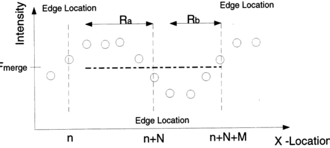
Region Merging
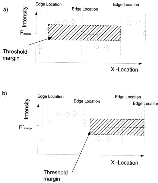
For region merging, the edge separating two adjacent regions is removed to merge them into a single region. This is done by taking the mean of the intensity values over the two adjacent regions that currently evaluate. For a horizontal scan, the mean of the intensity values within the examined regions is calculated as:
1 n+N+M
Fmerge N+M I( (3.1)
where j = j0 for each y-coordinate index of horizontal scan line
n= x-coordinate index of first pel in region,
N=total number of pels within leftmost region examined, M=total number of pels within rightmost region examined
Rb = {n + N + 1, n + N + 2,..., n + N + M} : rightmost region for j = jo
Figure 3-3 illustrates the parameters used in the region merging operation.
. L Edge Location Edge Location
SRa R C Fmerge --- ---0 0 I I Edge Location
n
n+N
n+N+M
X -Location
Figure 3-3: Diagram illustrating Mean Based merging parameters
The absolute deviation of the original intensity value from the mean intensity
value is calculated as:
A(i,j)
=
I(i, j)- Fmerge
1
(3.2)
where V(i,j)E
(R,U
Rb)In order to reduce the effect of noise, the third largest deviation value is selected
as the measure to compare with the pre-defined merging threshold. If the selected
deviation is less than the pre-defined merging threshold, the edge separating the
adjacent regions is removed to merge the two regions into one. If
A
3 > Mthresholdwhere
A3 isthe third largest deviation, and
Mthesholdis a pre-defined threshold, then
remove edge at (n + N, jo) to merge the two adjacent regions R., Rb
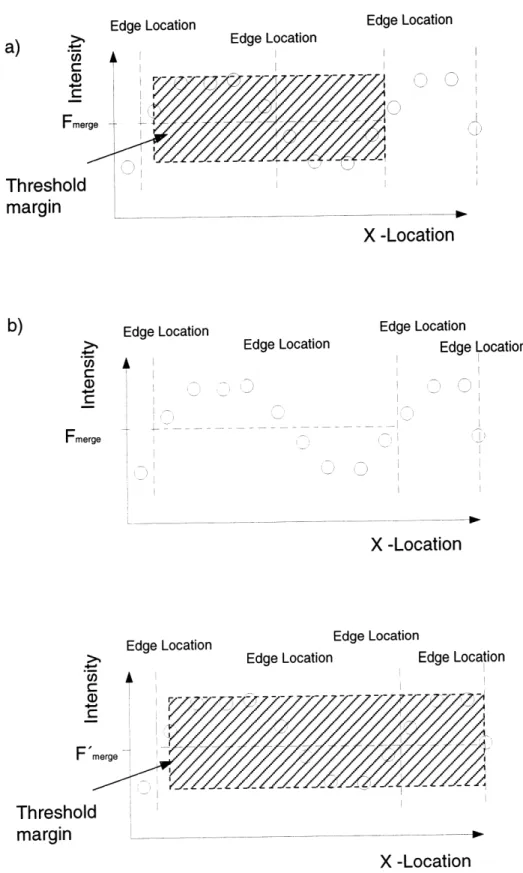
Edge Location Edge Location i VJ
X -Location
Edge Location4
Edge Location Edge Location Edge LocationX -Location
Edge Location Edge Location
Edge Location Edge Location
X -Location
Figure 3-4: 1-D illustration of Mean-based merging process. (a) Examined region has A3 < Mthreshold. (b) The edge dividing the two regions is removed. (c) The next step
examines the combined region and the next adjacent region.
.4-a Fme
Threshold
marain
FmergeF
Threshold
margin
Edge LocationEdge Location Edge Location
vi
X -Location
Edge Location Edge Location Edge Location Edge LocationX -Location
Threshold
margin
Figure 3-5: Merging process when threshold is exceeded. (a) Examined region has
A3 > Mthreshold.
(b) The next step examines the regions as illustrated.
a) FmEThreshoic
marain
F 'merge v Edge Locationof the merged region Rab = (Ra
U
Rb) and the next adjacent region. If the selecteddeviation is larger than the merging threshold, the edge is untouched and the process is repeated for the next two regions which are the later region Rb,and the next adjacent region. If
A3(i, j) <_ Mthreshold
then ignore edge at (n + N, jo)
Figure3-4 and 3-5 illustrate the details of the merging process based on the mean intensity value within adjacent regions.
3.2.2
Region Division
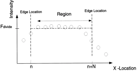
The region division operation examines a single region. The average of the intensity within the region is calculated as:
1 n+N (3.3)
Fdivide
= N E 1(',where j = j0 is the y-coordinate for each horizontal scan line
n=: x-coordinate of first pel in region,
N=total number of pels within single region
R = (n,n + 1, ... , N + N) : Region of interest
Figure 3-6 illustrates the parameters used in the region division operation.
The deviation of the intensity values from the mean value is subsequently calcu-lated as,
A(i, j) = I(i,j) - Fdivide (3.4)
Again, to reduce the probability of detecting noise-induced edges, the third largest deviation A3 within the region was chosen as the measure to compare with the pre-defined division threshold. If
A3 > Dthreshold (3.5)
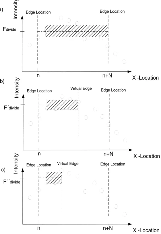
where Dthreshold is a predefined region division threshold, then place a virtual edge to divide the region into two temporary regions.
C,
a)
Edge Location Edge Location• .L,',reion F v Fdivide I I I I II
U 0
On
n+N
X -Location
Figure 3-6: Illustration of Region Division parameters
The virtual edge is placed as a flag to reference the boundary of the temporary
region. The process is recursively repeated on the leftmost region of the two divided
regions, until a divided region no longer has a A
s which is larger than the threshold.
3If
A3 < Dthreshold (3.6)
Replace the virtual edge with a real edge to divide the region. Ignore all previous
virtual edges. Then examine next adjacent region. The region division operation is
illustrated in figure 3-7 and 3-8.
There are several candidate points for the region division pel location. The
fol-lowing candidate region division points are examined.
Method A: Third largest deviation pel.
Method B: Leftmost pel that has a larger deviation than the threshold.
Method C: Pixel that has the largest gradient.
Edge Location Edge Location
-II
F-n+N
Edge Location Virtual Edge
9
X -Location
Edge Location
-1
n+N
X -Location
Edge Location Virtual Edge
I 7
Edge Location
I
I
n+N
X
-Location
Figure 3-7: 1-D illustration of Region Division operation. (a) Examined region hasA3 > Dthreshold. (b) Region is temporarily divided into two smaller regions by a virtual edge. Leftmost region is examined and A3 > Dthreshold. (c) Leftmost region is separated and virtual edge is placed. Previous virtual edge is ignored. Leftmost region is examined again where A3 < Dthreshold.
>1
a)
Fi--Fdivide Fdivide
b)
C)C
a)
F divide >,C"-c)
E
F "divide i , p md)
"C
Real Edgea) Edge Location Edge Location
F'
divideI 1r
I II
n
n+N
X -Location
Figure 3-8: Virtual edge is replaced with real edge and next adjacent region is exam-ined.
Method A
The A3 pel is readily selected when computing the measure to compare with the division threshold. Therefore, no further computation is necessary when selecting the region division pel location. The possibility of placing noise-induced edges is low because the two largest deviation points are ignored. However, the edge location is inconsistent from scan line to scan line and therefore, the continuity of the contours is poor resulting in a high total bit rate. The edge location is also inconsistent with the criterion used for the Sobel and Level edge based method, resulting in poor continuity between added edges and existing Sobel and Level based edges. Overall, using the
A3 pel as the division point produces a binary edge map with many short contours,
and the compression ratio is reduced.
Method B
Using the leftmost pixel that has a deviation larger than the set threshold divides the region at a point where the leftmost region already has a Delta3 less than the thresh-old. Therefore, this method arrives at a divided region which has A3 < Mthrehold in one division operation. The computation is reduced compared to Method A. How-ever, the regions are divided into the minimum widths that satisfy the thresholding
criterion and result in a high number of edges. The contour continuity is poor for the same reasons as discussed above for Method A.
Method C
If the region segmentation algorithm is used in conjunction with the Sobel and Level edge detection algorithm, the gradient is readily computed. The difference between this method and using a Sobel and Level edge method to obtain the edge from the gradient map, is that the criterion for choosing an edge as a region division point is dependent on the deviation of the entire region that we are examining. In the Sobel edge detection, the operation is local and only looks at the pixels within the 3x3 neighborhood of the local operator to calculate the gradient. The edges are then selected by a fixed global threshold for the entire image. The method proposed uses a more global criterion by incorporating all the pixels within a region contained between two adjacent edges to determine the validity of an edge. The continuity of the contours is improved over Method A and B. Successive edges occur next to existing edges where the gradients are large. A constraint needs to be placed around existing edges to prevent successive edges.
3.2.3
Problems with Mean-based region segmentation
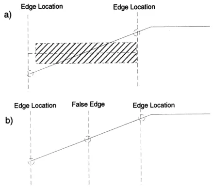
Problems occur with the mean based region segmentation method when intensity transitions in a region is slowly varying in a ramp like manner. The mean based method will add false edges at a slowly varying transition zone in the region division process. This is because the deviation from the mean value of the intensity within a region is exceeded as illustrated in figure 3-9.
Edge Location Edge Location
a)
Edge Location False Edge Edge Location
b)
Figure 3-9: Mustration of why Ramp-like behavior of intensity will cause placement
of region boundary in slow transition zone. (a) The intensity is slowly varying and
A > Dthreshd. (b)A false edge is
placedin the region division
process.3.3
Line fitting Approach
3.3.1
Motivation
As the mean based method for one-dimensional spatial intensity region division can
not adapt to intensities that are slowly varying in a ramp like manner, we proposed
a
method that would be based on line-fitting. By using the deviation from an intensity
fitted line as a basis for region segmentation criterion, we can reduce the detection
of false edges that occur in slowly varying intensities when using the mean based
method. Another important advantage of using line fitting in the region segmentation
operation is the consistency with the reconstruction process, as the reconstruction
process is based on linear interpolation. The line-fitting approach can encode
the
image by producing a binary edge map where regions have an optimized width
for
linear interpolation. The computational load is heavier than the mean-based approach
because of the calculations required to fit a line to the intensity values in a region.
Since various closed form functions for data line-fitting are available, we used a method
described in the "Numerical Recipies".
Again we considered several approaches for segmenting the regions. The region merging and region division processes are discussed in separate sections. Under the region division process, several options for selecting the point of region division are
examined.
3.3.2
Region merging
Region merging is done in the following order. Take the Mean Absolute Error (MAE) of the estimated intensity line fitted value from the original intensity value within two successive regions along a scan line. If the MAE is less than the set merging threshold, remove the edge separating the two regions to merge them into one region. If the two regions are merged, the same operation is repeated on the combined region and the next region along the scan line. If the two regions are not merged, the next two regions examined include the second region along the scan line that was incorporated in the previous merging operation and its following region. The region merging process is applied to both horizontal and vertical scan lines and the resulting combined edge map is obtained by the logical OR product of the two binary edge maps. figure3-10 explains the merging process.
1 n+N+M
MAEinefit
N
A(i,j)
(3.7)i=n
given that n = leftmost pel of regions,
N = total number of pels in leftmost region, M = total number of pels in rightmost region,
A(i,j) = ]I(i,j) - I(i, j
where I(i,
j):
line fitted estimate of intensity data3.3.3
Region Division
In this section the various methods of dividing regions to obtain a binary edge map are examined. The main objective of the region division process is to obtain regions
Edge Location
ci)
rThreshold
margin
Edge LocationX -Location
Edge Location0
C0
Edge Location Edge Location Ir
IQI0
0
X -Location
Edge Location Edge Location
Edge Location
X -Location
Figure 3-10: Illustration of line-fitted region merging process
C)
Threshok
margin
Edge Locationa
t
I vin which the original image intensity map can be best represented by one dimensional
linear interpolation. The possibility of using only a vertical or a horizontal scanned
binary edge map were considered in order to reduce the total bits required to represent
the reconstructed image. However, results of reconstructing the image from edge
maps produced from a one directional scan were poor, because of the weak contour
definition in the other direction. The results for each region division method are
discussed below in each of their sections respectively.
Method A
Divide the region at the leftmost encountered pel where the deviation between the
original intensity and the line-fitted value is larger that the pre-defined region division
threshold. The process scans the divided region recursively, until the region has no
deviations larger than the division threshold. Continuity of the contours are poor
due to the inconsistency in edge location from scan line to scan line. When used in
conjunction with the Sobel and Level Edge detection method, the added edges has
poor continuity with the existing edges. Short broken contours are produced, leading
to an increase in the total bit rate.
Method B
The third largest deviation is used as the measure to compare with the division threshold. The region is divided at the third largest deviation pel location. The results for this algorithm showed short broken contours as in Method A. The edge location is not consistent from scan line to scan line and results in poor continuity.
Method C
The third largest deviation is used as the measure to compare with the division threshold. The region is divided at the largest gradient pel location. When used in conjunction with the Sobel and Level Edge method, the gradients are readily computed. The detected contour continuity using region segmentation is improved over Method A and B.
Method D
The Mean Absolute Error (MAE) of the intensity line fitted value to the original intensity value is used as the measure to compare with the division threshold. If the MAE is larger than the set division threshold, divide the region at the point of the largest gradient within the region. The computational load is high for calculating the
MAE.
Method E
Region growing method. Initially start with the first pixel along the scan line as a region. Grow the region one pixel at a time. For every step, compute the fitted line. If the region at the current step ends at N, Calculate the deviation of the original intensity to the estimated next intensity value using the parameters of the fitted line at N+1. If the deviation is larger than the set division threshold, segment the region at the spatial value N. Repeat the process starting at N+1. The optimum region width that satisfies the region division threshold is obtained. However, the contour continuity is poor and the computational load is very high.
3.3.4
Thinning of thick edges
With no constriction on placing edges successively along a scan line, several areas have edges occuring in succession. This is because the gradient is large for several pixels around edges. Successive edges increase the total bit rate. Ideally, the contours should be a single pixel wide. To avoid successive edges from occuring, various methods are examined.
The first method is to post process the successive edges based on the following approaches
1. Take the midpoint of the successive edges, and remove all the other edges.
2. Leave the two edges on both sides of the successive edges and remove all the edges in between.
Method 2 divides the regions into smaller regions that are better represented by
line fitted intensity values. The characteristics of the original image intensity map are
better represented within the region of the successive edges, than the region between
the edge prior to the successive edges and the mid point of the successive edges.
However, the number of edges resulting from the thinning operation is twice that of
Method 1. Figure 3-11 illustrates these thinning approaches.
a) F I
I I I I
b)
F F IFigure 3-11: Illustration of thinning of successive edges. (a) Edges placed in
succes-sion. (b) Thin by removing all edges in between end-edges. The resulting regions
produce a better fitted line. (c) Thin by removing all edges except midpoint edge.
The remaining edge is half that of the method (b), however the fitted lines have a
larger error.
The simplest approach that requires less computation is to place a restriction on
the detection of edges by using a larger threshold for several pixels after an edge
prdc abterFte lieFc Thnb rmvn al de Fxetmdon deFh
eann dei hafta oftemto (bhwvrteFitdlnshva
FarFr
eror
Fh
ipetapoc Fhtrqie Fescmuaini opaearsrcino
Fh
detection. This would avoid edges occuring in succession prior to their detection. The algorithm eliminates the possibility of placing a new edge next to an originally detected edge.
3.4
Continuity Issues
This section is concerned with the problem of contour continuity. The total bit rate depends directly on the number of the distinct contours and the number of contour pixels through the equation expressed in [2]:
NM
1.3Lc + 41Nc +
NM
(3.8)where Lc is the total number of edge pixels, Nc is the number of distinct contours, and N x M is the image size.
The above equation indicates that the number of distinct contours weighs more into the total bit rate. Therefore, to obtain a high compression rate, ideally, the contours should be long and continuous with as few breaks as possible.
3.4.1
Breaks in contours
If region segmentation is computed over one dimensional scan lines, breaks occur in the generated contours. In order to overcome this problem, the intensity character-istics of the neighboring scan lines can be incorporated into the region segmentation process. To facilitate this approach, a hint was obtained from the 3x 3 Sobel gradient operator. The Sobel operator is quite effective in generating edge maps with contin-uous contours. In the proposed approach, we use the intensity data within a region along a scan line. Instead of using the intensity data along a one-dimensional scan line, a weighted sum of three consecutive lines including the current, upper and lower intensity data will result in better continuity from scan line to scan line because of the overlap in incorporated intensity data in the region segmentation process. The weighting of the intensity data is chosen empirically. For each pel, the weighted sum
value is calculated by:
I(i, N - 1) + 2 x I(i, N) + I(i, N + 1)
(iN)
(3.9)= Ic (i, N)
(3.9)
4
where I(i,j) is the intensity value of the pixel. N is the current scan line.
-.
0 I(i,N-1)o
line N-1
line N
(i,N+)
(i,)
Line N+1
X-coordinate
Figure 3-12: Illustration of pels used in weighted intensity calculation
This modification improves the compression ratio by limiting the number of short breaks in the middle of long contours.
3.4.2
Modifications in the thinning operation
In the original method of edge detection, a thinning operation is performed on the Sobel and Level edge generated edges to obtain single pixel wide contours. The objective of the proposed method is to improve the quality of edge detection and possibly fill in the imperfections that occur in the contours. If the proposed method is to be used as a post process to the original edge detection operation, continuity must be maintained between the originally detected edges and the additionally detected edges through region segmentation.
An elementary approach to maintain continuity is to select region boundaries through the same thinning operation performed in the original algorithm. If the region segmentation algorithm does not detect a pixel that satisfies the criterion within the region, the pixel with the highest gradient obtained through the Sobel operator is selected as the region boundary pixel. The difference in the original edge
detection operation and the proposed method is that the edge placement is dependent on the intensity data analyzed within a region, instead of limiting the selected edges to pixels that have Sobel gradients larger than a fixed threshold. Therefore, although the same thinning criterion is used to select edges, the proposed method places edges depending on the local characteristics within the region, in comparison to the original method that uses a fixed threshold for the entire image to create a binary edge map.
U
C
r
d
Figure 3-13: Pels used in thinning method. c, u, d, 1 and r represent the gradients at the current, up, down, left and right pixels, respectively.
Select the pixel that satisfies:
[c> u AND c > d AND c> IAND c > r] OR
[(c > u AND c > d AND I > I ) OR (c > lAND l c AND c>rANDI > I]
Where I, is the horizontal gradient and I, is the vertical gradient of the current pel. If none of the thinning criterions are satisfied within the region, select the pel that has the maximum gradient.
3.4.3
Problems with Contour Filtering
The contour filtering algorithm searches for the start point of a contour line from top to bottom, and left to right of the image. The algorithm then follows the contour in a clockwise direction.
Branching Effects on Edge Placement
Problems occur with the contour filtering algorithm, when a contour branches into several contours. The algorithm follows the contour that branches off in the clos-est clockwise direction. This is independent of the contour length of the branches. Therefore, if an edge is added through region segmentation that results in a branch off a long contour, the originally long contour is possibly divided at the branch point into a shorter contour. Figure 3-14 illustrates the result of an added edge from region division along the X-direction resulting in a branch. The figure shows that because of the additional edges placed, the long contour is segmented into shorter contours and removed through the contour filtering process when its length is less than the set minimum contour length.
In order to avoid this problem a constraint needs to be applied on the conditions for edge placement. A possible constraint is to detect that an added edge would cause a branch in a contour prior to placing the edge.
Problems with Curved Contours
Another problem with the algorithm happens when a contour curves with a peak towards the top of the image. The contour filtering algorithm detects the peak as the starting point of the contour. If the contour is not an enclosed loop, the contour filtering algorithm counts the curved contour as shorter contours divided at the peak. An example is illustrated in figure 3-15.
The binary edge map shows the originally continuous contour at the top of the eye, being removed through the contour filtering process with a minimum contour length of 7. This is because the length of the contour representing the eyelid is counted as 2 shorter contours by the algorithm, where one is shorter than the minimum allowed contour length.
Added edge through region division
Original contour
--0
(a)
X-coordinate
F77?7777;.:~
(b)
X-coordinate
(c)
X-coordinate
Figure 3-14: Branching causing different results after contour filtering (a) Edge is added through region division that results as a branch from the original contour. (b)The contour is counted by the contour filtering algorithm as two shorter contours. (c) The shorter contour is now removed through the filtering process.
&
.
..I
(a)
(b)
Figure 3-15: Problems with curved contours with peaks towards the top of the image
3.4.4
Region width
The intensity characteristics of 2 adjacent pixels in the original image can be perfectly replicated using linear interpolation in the reconstruction process. To allow for a margin of error, the minimum region width is limited to 3 pixels. Therefore, in the region division process, if the region examined has a width greater than 6 (2 minimum region widths), the region is not divided any further. Also, additional edges are not placed if within 3 pixels distance from an original contour along the scan line direction.
3.5
Intensity coding
The intensity coding process is done by encoding the intensity to the right of an edge pixel and the intensity for the following edge pixel. In our representation the interpolated line is obtained from incorporating the intensity values for pixels within an entire region. This differs from the method used in [2] where the few pixels adjacent to an edge pixels are ignored to obtain a fitted line representing the "relevant data" by ignoring the pel intensity values which are too close to the contours within the region.
In our method, the fitted line represents the original data more accurately since all the intensity data within a region is incorporated in calculating the fitted line. This results in a better reconstructed image that does not have the large distortion as seen in [2] close to the contours, due to the data ignored in close proximity to the contours. In [2], the intensity is coded by averaging the intensity values that overlap in the horizontal and vertical intensity coding. This results in a distortion of the intensity values later used in interpolating the intensity data due to the difference of the hor-izontal and vertical intensity values representing the same pixel. If the overlapping intensity values of the pixels used in both the horizontal and vertical scanning, are encoded separately for the horizontal and vertical interpolation, the image quality is enhanced by producing more accurate reconstructed intensity values. However, for the "Lenna" image the overlapped pels amounted to 2270. With 4 bits assigned to pel, the overall bit rate increases by approximately 50%. Therefore, this intensity coding method was discarded.
The intensity values along a contour are then averaged over a pre-defined number of pixels along a contour. The method of intensity coding along a contour is explained
in [2].
3.6
Encoder Block Diagram
The complete block diagram of the color encoder is shown in figure 3-16. The input is a color static image in the YIQ format. The Edge detection and Region Segmentation operations are performed on the luminance (Y) component alone.
Edge Detection Region Division
4Y
Y
Intensity Extraction ,- Intensity Coding
YIQ
Mean Coding .
Figure 3-16: Block Diagram of Color Static Encoder using Region Segmentation
Input Image
Chapter 4
Performance Results
4.1
Performance and Results
Improving the subjective image quality for a fixed compression rate is the main objec-tive in developing the region segmentation approach. In analyzing the performance results, it is difficult to come up with a quality criterion that will directly reflect the psycho-visual properties of image interpretation. However, to quantify the distor-tion of the reconstructed image, Peak to Signal noise ratio (PSNR) will be used in this thesis as a measure to compare the results of the various region segmentation methods.
4.2
Results
This chapter discusses the results of the proposed algorithm using Region segmenta-tion in comparison to the original Sobel and Level Edge based method.
4.2.1
Region segmentation without Sobel and Level edge
detection
In this section the results of the Region segmentation program when used alone to produce the binary edge map are discussed. The produced binary edge map has a
reduced total number of edge pixels for the same image quality in PSNR, however there are breaks in contours, reducing their continuity which leads to a higher total bit rate. For the same total bit rate, the image quality was subjectively poor due to the lack of edge pixels in the binary edge map.
4.2.2
Hybrid method of Sobel and Region Segmentation
The Region segmentation approach, when used in conjunction with the Sobel and Level Edge operation, produced the best results. The region segmentation method using the line-fitting approach and Method C described in 3.3.3 is used to produce the results discussed in this section. In the region segmentation operation, the Mean Absolute Error (MAE) of the linearly interpolated intensity value to the original image intensity value is used in the region evaluation process. Therefore, the breaks in contours occur where the MAE or the 'fit' of the interpolated intensity satisfies the set criterion. The smearing effect around these breaks is therefore less significant than what is produced in the original algorithm.
When using the region segmentation operation on the binary edge map produced by the Sobel and Level edge operation, the gaps that lead to unpleasant line artifacts can be filled in a more efficient manner than lowering the Sobel and Level edge threshold. The comparison is shown in figure 4-1.
(a)
(b)
Figure 4-1: (a)Binary edge map with low Sobel threshold of "Lenna" at 0.275 bpp.(b)Binary edge map using hybrid method at 0.270 bpp.
(a)
(b)
Figure 4-2: (a)Interpolated image (without mean coding) of "Lenna" using original algorithm at 0.275 bpp. (b) Interpolated image (without mean coding) of "Lenna" using proposed algorithm at 0.270 bpp. There is less smearing of the image especially around the pillar to the left of the image.
(b)
Figure 4-3: (a)Reconstructed image (with mean coding) of "Lenna" using original algorithm at 0.275 bpp. (b) Reconstructed image (with mean coding) of "Lenna" using proposed algorithm at 0.270 bpp. The definition of the pillar to the left of the image is improved.