The economic impacts of climate change : evidence from agricultural profits and random fluctuations in weather

Digitized

by

the

Internet

Archive

in

2011

with

funding

from

Boston

Library

Consortium

Member

Libraries

DEWEY

u

+15

.6M"

-6

Massachusetts

Institute

of

Technology

Department

of

Economics

Working

Paper

Series

The

Economic

Impacts

of

Climate

Change:

Evidence from

Agricultural

Profits

and

Random

Fluctuations

in

Weather

Olivier

Deschenes

Michael

Greenstone

Working

Paper

04-26

July

2004

Room

E52-251

50

MemorJal

Drive

Cambridge,

MA

021

42

This

paper can be

downloaded

without

charge from

the Social

Science

Research

Network

Paper

Collection at

MASSACHUSETTS

INSTITUTE

OF

TECHNOLOGY

DEC

7

20M

The Economic

Impacts

of

Climate

Change:

Evidence

from

Agricultural

Profits

and

Random

Fluctuations

in

Weather*

Olivier

Deschenes

University

of

California, Santa

Barbara

Michael Greenstone

MIT

and

NBER

July

2004

*

_We

_thank

_David

_Bradford

_{for initiating a conversation that ultimately led to this paper.}

_Hoyt

Bleakley,

Tim

Conley,

Enrico

Moretti,

Marc

Nerlove,

and

Wolfram

Schlenker

provided

insightful

comments.

We

are also grateful for

comments

from seminar

participants at

Maryland,

Yale, the

NBER

Environmental

Economics

Summer

Institute,

and

the

"Conference on

Spatial

and

Social Interactions in

Economics"

at the University

of

California-Santa Barbara.

Anand

Dash,

Barrett

Kirwan,

Nick

Nagle,

and

William

Young,

provided

outstanding research

assistance. Finally,

we

are indebted to

Shawn

Bucholtz

at the

United

States

Department of

Agriculture for

generously

generating the

weather

data.

Greenstone

acknowledges

generous

The

Economic

Impacts

of

Climate

Change:

Evidence

from

Agricultural

Output and

Random

Fluctuations

in

Weather

ABSTRACT

This

paper measures

the

economic

impact of

climate

change

on

US

agricultural land.

We

replicate the previous literature's

implementation

of

the

hedonic

approach

and

find that it

produces

estimates

of

the effect

of

climate

change

that are

very

sensitive to decisions

about

the

appropriate control variables,

sample

and

weighting.

We

find estimates

of

the

benchmark

doubling

of greenhouse

gases

on

agricultural land values that

range

from

a decline

of $420

billion

(1997$)

to

an

increase

of

$265

billion, or

-30%

to

19%.

Despite

its theoretical appeal,

the

wide

variability

of

these estimates suggests thatthe

hedonic

method

may

be

unreliablein this

setting.

In light

of

the potential

importance

of

climate

change,

this

paper

proposes

a

new

strategy to

determine

its

economic

impact.

We

estimate the effect

of weather

on

farm

profits, conditional

on

county

and

state

by

year

fixed effects, so the

weather parameters

are identified

from

the

presumably

random

variation in

weather

across counties within states.

The

results

suggest

that the

benchmark change

in climate

would

reduce

the value

of

agricultural land

by

$40

to

$80

billion, or

-3%

to

-6%,

but the null

of

zero effect

cannot

be

rejected. In contrast to the

hedonic

approach,

these results are robust to

changes

in specification.

Since farmers can

engage

in a

more

extensive set

of

adaptations in

response

to

permanent

climate changes, this estimate is

likely

downwards

biased, relative to the preferred long run effect.

Together

the point estimates

and

sign

of

the likely bias contradict the

popular

view

that climate

change

will

have

substantial

negativewelfare

consequences

forthe

US

agricultural sector.

Olivier

Deschenes

Department of

Economics

2127

North

Hall

University

of

California

Santa

Barbara,

CA

93106-9210

email: olivier(2)econ.

ucsb.edu

Michael Greenstone

MIT,

Department

of

Economics

50

Memorial

Drive,

E52-391B

Cambridge,

MA

02142

and

NBER

Introduction

There isa

growing

consensusthatemissions of greenhousegases dueto

human

activity will lead

tohighertemperaturesand increasedprecipitation. It is thoughtthatthesechangesinclimatewill impact

economic

well being. Since temperature and precipitation are direct inputs in agricultural production,

many

believethatthe largest effects willbe in thissector. Previousresearch onthe

benchmark

doubling

of atmospheric concentrations ofgreenhouse gases is inconclusive about the sign and

magnitude

ofits

effect

on

the value of

US

agricultural land

(Adams

1989;

Mendelsohn,

Nordhaus, and

Shaw

1994 and

1999; Schlenker,

Hanemann,

andFisher 2002).

Most

previous research

employs

eitherthe production function or hedonic approach to estimate

theeffectofclimatechange.1

Due

toits experimental design, the productionfunction approach provides

estimates of the effect of weather

on

the yields of specific crops that are purged of bias

due

to

determinantsofagricultural outputthatare

beyond

farmers' control(e.g., soilquality). Itsdisadvantageis

thatthese experimental estimates do notaccountforthe full rangeof compensatoryresponsesto changes

in weather

made

by profit

maximizing

farmers. For

example

in responseto achange in climate, farmers

may

alter their use of fertilizers,

change

their

mix

ofcrops, or even decide to use their farmland for

another activity (e.g., a housing complex). Since farmer adaptations are completely constrained in the

production function approach, it is likely to produce estimates of climate change that are biased

downwards.

The

hedonicapproach attempts to

measure

directly theeffectofclimate on landvalues. Its clear

advantage isthat ifland marketsare operating properly,prices will reflectthe presentdiscountedvalueof

land rents into the infinite future. In principle, this approach accounts for the full range of farmer

adaptations.

The

limitationisthatthevalidityofthisapproach requires consistentestimationoftheeffect

ofclimate on landvalues. Sinceat leastthe classic

Hoch

(1958 and 1962) and

Mundlak

(1961)papers, it

has been recognized that

unmeasured

characteristics (e.g., soil quality) are an important determinant of

output and land values in agricultural settings.2 Consequently, the hedonic approach

may

confound

climatewithotherfactorsandthesignand magnitude oftheresultingomittedvariables bias is

unknown.

In light ofthe importance ofthe question, this paper proposes a

new

strategy to estimate the

effects ofclimate change on the agricultural sector.

We

use a county-level panel data file constructed

from the Censuses ofAgriculture to estimatethe effect of weather

on

agricultural profits,conditional on

1

Throughout

"weather" refers to the state ofthe atmosphere at a given time and place, with respectto

variables such as temperature and precipitation. "Climate" or "climate normals" refers to a location's

county and state by year fixed effects. Thus, the weather parameters are identified from the

county-specific deviations in weather about the county averages after adjustment for shocks

common

to all

counties in a state. This variation is

presumed

to be orthogonal to unobserved determinants of

agriculturalprofits, so it offers a possible solution tothe omitted variables bias problems that appear to

plaguethehedonic approach. Its limitation isthatfanners cannot

implement

thefull range ofadaptations

in response to a single year's weather realization, so its estimates ofthe impact ofclimate

change

are

biased

downwards.

Our

analysis begins with a reexamination ofthe evidence

from

the hedonic method.

There

are

two

important findings. First, the observable determinants of land prices are poorly balanced across

quartiles of the long run temperature

and

precipitation averages. This

means

that functional form assumptions are important in thisapproach. Further, it

may

suggestthat unobserved variables are likely tocovary withclimate.

Second,

we

replicate the previous literature's implementation of the hedonic approach

and

demonstratethat it produces estimates ofthe effect ofclimate

change

thatare very sensitive todecisions

aboutthe appropriate control variables,sample and weighting.

We

find thatestimatesoftheeffectofthe

benchmark

doubling of greenhouse gasses

on

the value of agricultural land range

from

-$420 billion

(1997$) to

$265

billion (or

-30%

to 19%),

which

is an even wider range than has been noted in the

previousliterature. Despite its theoretical appeal, the

wide

variability ofthese estimates suggests thatthe

hedonic

method

may

beunreliablein thissetting.3

The

results

from

our preferred approach suggest that the

benchmark

change in climate

would

reduceannualagricultural profitsby $2 to$4 billion,but thenull effectofzerocannotberejected.

When

thisreduction in profits is

assumed permanent

anda discount rateof

5%

isapplied,theestimates suggest

that the value ofagricultural land is reduced

by

$40

to

$80

billion, or

-3%

to

-6%.

Notably,

we

find

modest

evidencethat farmersare abletoundertake a limitedset ofadaptations (e.g., increased purchases

offeed, seeds, and fertilizers) in response to weather shocks. In the longer run, they can engage in a

wider variety ofadaptations, so our estimates are

downwards

biased relative to the preferred long run

effect. Together the point estimates and sign ofthe likely bias contradict thepopular

view

that climate

changewillhavesubstantialnegativeeffects

on

the

US

agricultural sector.

"

_Mundlak

_focused

_on

_{heterogeneity in the skills of farmers,}

_however

_{he recognized that there}

are

numerous

other sources offarm-specific effects. In

Mundlak

(2001), he writes,"Other sourcesof

farm-specific effects aredifferencesin landquality, micro-climate,

and

so

on"

(p. 9).

This finding is consistent with recent research indicating that cross-sectional hedonic equations are

misspecified in a variety ofcontexts(Black 1999; Blackand Kneisner 2003;

Chay

and Greenstone 2004;

In contrast to the hedonic approach, these estimates ofthe

economic

impact ofglobal

wanning

are robust. For example, the overall effect is virtually

unchanged

by adjustment for the rich set of

available controls,

which

supports the assumption that weather fluctuations are orthogonal to other

determinants of output. Further, the qualitative findings are similar whether

we

adjust for year fixed

effects or state

by

year fixed effects (to control for unobserved time-varying factors that differ across

states). Thisfindingsuggests thattheestimates aredueto outputdifferences, not price changes. Finally,

we

find substantial heterogeneity in the effect ofclimate change across the United States.

The

largest

negative impacts tend to be concentrated in areas of the country

where

fanning requires access to

irrigationand fruits andvegetables arethepredominantcrops(e.g.,CaliforniaandFlorida).

The

analysis is conducted with the

most

detailed

and

comprehensive data available on

agricultural production, soil quality, climate, and weather.

The

agricultural production data is derived

from the 1978, 1982, 1987, 1992, and 1997 Censuses ofAgriculture andthe soilquality data

comes

from

theNational ResourceInventory datafilesfromthe

same

years.

The

climateand weatherdataare derived

fromtheParameter-elevation Regressions on Independent Slopes

Model (PRISM).

This

model

generates

estimates ofprecipitation and temperature at small geographic scales, based

on

observations

from

the

more

than 20,000 weather stations in the National Climatic Data Center's

Summary

of the

Month

Cooperative Files during the 1970-1997 period.

The

PRISM

data are used by

NASA,

the

Weather

Channel, and almostallother professional weatherservices.

The

paperproceeds asfollows. Section I motivatesourapproach anddiscusses

why

it

may

be an

appealing alternative to the hedonic and production function approaches. Section II describes the data

sourcesandprovides

some

summary

statistics. Section IIIpresents theeconometric approachand Section

IV

describes the results. Section

V

assesses the

magnitude

of our estimates ofthe effect of climate

change anddiscusses a

number

ofimportant caveatstothe analysis. Section

VI

concludesthepaper.

I.Motivation

This paper attemptsto develop areliable estimate oftheconsequences ofglobal climate change

inthe

US

agricultural sector.

Most

previous research onthistopic

employs

eithertheproductionfunction or hedonic approach to estimatethe effect ofclimate change. Here,

we

discuss these methods' strengths

and weaknessesand motivate ouralternativeapproach.

A. Production Function

and Hedonic Approaches

to ValuingClimate

Change

The

production function approach relies on experimental evidence ofthe effect of temperature

provides estimates ofthe effectof weather on the yields ofspecific crops that are purged ofbias dueto

determinantsofagricultural outputthat are

beyond

farmers' control (e.g., soil quality). Consequently, it

is straightforward to use the results ofthese experiments to estimate the impacts ofa given

change

in

temperatureorprecipitation.

Its disadvantageis thatthe experimental estimates areobtained in alaboratory setting

and

donot

accountfor profit

maximizing

farmers'

compensatory

responsesto changes in climate.

As

an illustration,

consider a permanent and unexpected declinein precipitation. Inthe short run, farmers

may

respond by

increasing the flow of irrigated water or altering fertilizer usage to mitigate the expected reduction in

profits

due

tothedecreased precipitation. Inthe

medium

run, farmers canchooseto plant differentcrops

that require less precipitation.

And

in the long run, farmers can convert their land into housing

developments, golf courses, or

some

other purpose. Since even short run fanner adaptations are not

allowed intheproduction function approach, it producesestimates ofclimate change that are

downward

biased. Forthisreason,itis

sometimes

referredto asthe

"dumb-farmer

scenario."

In aninfluentialpaper,

Mendelsohn,

Nordhaus, and

Shaw

(MNS)

proposed the hedonic approach

as a solution to the production function's shortcomings

(MNS

1994).

The

hedonic

method

aims to

measure

the effectofclimate

change

by

directlyestimating theeffectof temperature andprecipitation

on

thevalue ofagricultural land. Itsappeal is that ifland markets are operating properly, priceswill reflect

the present discounted value ofland rents into the infinite future.

MNS

write the following about the

hedonic approach:

Instead of studyingyields

of

specific crops,

we

examine

how

climate in differentplaces

affects thenet rentor value

_of

farmland.

By

directly

measuring

farmprices orrevenues,

we

account for the direct impacts

of

climate on yields ofdifferent crops as well as the

indirect substitution

of

different inputs, introduction

_of

different activities,

and

other

potentialadaptationsto differentclimates (p. 755, 1994).

Thus

the hedonic approach promises an estimate ofthe effect ofclimate

change

that accounts for the

compensatory

behaviorthatunderminestheproductionfunctionapproach.

To

successfully

implement

the hedonic approach, itis necessaryto obtain consistent estimates of

the independent influence ofclimate

on

landvalues andthis requiresthat all unobserved determinants of

landvaluesareorthogonal toclimate.4

We

demonstrate

below

thattemperature andprecipitation normals

covary with soil characteristics, population density, per capita income, latitude, and elevation. This

means

that functional form assumptions are important in the hedonic approach and

may

imply that

In Rosen's (1974) classical derivation ofthe hedonic model, the estimates ofthe effect ofclimate

on

land prices canonly be usedto valuemarginalchanges in climate. It is necessarytoestimatetechnology

parameters to obtainvalue non-marginal changes.

Rosen

suggests doing this ina second step. Ekeland.

Heckman,

and

Nesheim

(2004) outline a

method

to recover these parameters in a single step.

MNS

implicitly

assume

thatthe predicted changes intemperature andprecipitationunderthe

benchmark

global

unobserved variables are likely to covary with climate. Further, recent research has found that cross-sectional hedonic equations appeartobe plagued

by

omittedvariables bias in avariety ofsettings (Black

1999;Black and Kneisner 2003;

Chay

and

Greenstone 2004; Greenstone and Gallagher2004).5 Overall,

it

may

be reasonableto

assume

thatthe cross-sectional hedonicapproach confoundsthe effect

of

climate

withotherfactors(e.g., soilquality).

This discussion highlights that for different reasons the production function and hedonic

approaches are likely to produce biased estimates of the

economic

impact of climate change. It is

impossible to

know

the

magnitude

ofthe biases associated witheitherapproach and in the hedonic case

even thesignis

unknown.

B.A

New

Approach

to ValuingClimate

Change

Inthispaper

we

propose analternative strategy toestimatethe effectsofclimatechange.

We

use

a county-level panel data file constructed

from

the Censuses ofAgriculture to estimate the effect of

weather

on

agricultural profits, conditional

on

county and state

by

year fixedeffects. Thus, the weather parameters are identified from the county-specific deviations inweather about the county averages after

adjustment forshocks

common

to all counties in a state. This variation is

presumed

tobe orthogonal to

unobserved determinants ofagricultural profits, so it offers a possible solution to the omitted variables

biasproblemsthatappeartoplaguethehedonicapproach.

This approach differs from the hedonic one in a

few

key ways. First, under an additive

separability assumption, its estimated parameters are purged ofthe influence of all unobserved time

invariant factors. Second, it is not feasible to use land values as the dependent variable oncethe county

fixed effects are included. This is because landvalues reflect longrun averages ofweather, not annual

deviations

from

theseaverages, andthereis no timevariation insuchvariables.

Third, although the dependent variable is not land values, our approach can be used to

approximatethe effectofclimatechangeon agriculturallandvalues. Specifically,

we

use the estimatesof

the effect of weather onprofits and the

benchmark

estimates ofauniform 5degreeFahrenheit increase in

temperature and

8%

increase in precipitation to calculate the expected

change

in annual profits

(IPCC

1990;

NAS

1992). Since the value ofland is equal tothe present discounted stream ofrental rates, it is

straightforward to calculate the change inland values

when

we

assume

thepredicted change in profits is

permanent

and

make

anassumption aboutthe discountrate.

5

For example, the regression-adjusted associations

between

wages

and

many

jobamenities and housing

prices andair pollution are

weak

andoften havea counterintuitive sign (Blackand Kneisner 2003;

Chay

Before proceeding, itis importantto clarify

how

shortrun variation in weatheraffects the profits

ofagricultural producers

and

under

which

conditionsthis variation canbe used to

measure

the effects of

climate change. Consider the following simplified expression for the profits of a representative

agriculturalproducer:

(1) 7i

=

p(q(w))q(w)

-

c(q(w)),

where

p, q,andc, denoteprices, quantities, andcosts,respectively. Pricesandtotalcosts areafunction of

quantities. Importantly, quantities are a function ofweather, w, because precipitation and temperature

directly affect yields.

Now

consider

how

the representativeproducer'sprofitsrespondtoachange inweather:

(2)

d%

1

3w

=

(dpIdq) (dq1

dw)

q

+

(p

-

3c/<5w)dqIdw.

The

first term is the

change

in prices due tothe weather shock (through weather's effect on quantities)

multipliedbytheinitial level ofquantities.

The

second termis thedifference

between

priceand marginal

cost multipliedby the

change

inquantitiesduetothechange inweather.

Sinceclimate

change

isa

permanent

phenomenon,

we

would

liketo isolatethe longrun

change

in profits. Consider the difference

between

the first term in equation (2) in the short

and

long run in the

contextofachangeinweatherthatreduces output. Intheshortrun, supplyislikely to beinelastic (dueto

the lag

between

planting

and

harvests),

which

means

that(dpI5q)shortRun

>

0. This increaseinprices will

helptomitigatefarmers' lossesduetothe lowerproduction.

However,

thesupplyofagricultural

goods

is

more

elastic inthe long run, so it is sensibleto

assume

that (dp I3q)Long Run is smaller in

magnitude

and perhaps even equal to zero. Consequently,the firstterm

may

be positive inthe short run but small, or

zerointhe longrun.

Although our empirical approach relies

on

short run variation in weather, it

may

be feasible to abstract

from

the change in profitsdueto pricechanges (i.e., the first term). Recall, the price level is a

functionofthetotalquantityproduced intherelevantmarketina givenyear.

By

usingapanelof

county-level data and including county and state by year fixed effects,

we

rely on across county variation in

county-specific deviations in weather within states. This

means

that our estimates are identified from

comparisons ofcounties that had positive weather shocks with ones that

had

negative weather shocks,

within the

same

state. Put inanotherway,thisapproachnon-parametrically adjusts forall factors thatare

common

across counties within a state by year, such as crop price levels. Ifproduction in individual

counties affectsthe overall price level,

which

would

bethe case ifa

few

counties determine cropprices,

or there are

segmented

local marketsfor agricultural outputs,then this identificationstrategy will notbe

abletoholdprices constant.

The

assumption that our approach fully adjusts for price differences

seems

reasonable for

most

across the country and not concentrated in a small

number

ofcounties. For example,

McLean

County,

Illinois and

Whitman

County,

Washington

arethe largest producers ofcorn and wheat, respectively, but

they only account for

0.58%

and

1.39%

oftotal productionofthese crops inthe

US.

Second, our results

are robust to adjusting for price changes in a

number

of different ways. In particular, the qualitative

findings are similarwhether

we

control forshocks with yearorstateby yearfixed effects.6

Returning to equation (2), consider the second term,

which

is the change in profits

due

to the

weather-inducedchangeinquantities.

We

would

liketoobtainanestimateofthistermbasedon longrun

variation in climate, sincethis is theessenceofclimate change. Instead, ourapproach exploits short run

variation in weather. Since farmers have a

more

circumscribed set ofavailable responses to weather

shocks than tochanges inclimate, it

seems

reasonable to

assume

that (3c /_3q)short

_r«

>

(3c/ _{3q)Long Run}.

7

For example, fanners

may

be able to change a limited set of inputs (e.g., the

amount

of fertilizer or

irrigation) in responseto weathershocks.

But

in responseto climate change, they canchange theircrop

mix

and even converttheir landtonon-agricultural uses (e.g.,tracthousing). Consequently,our

method

to

measure

theimpactofclimatechange islikely tobe

downward

biasedrelativetothepreferred longrun

effect.

In

summary,

the use of weather shocks to estimate the costs ofclimate change

may

provide an

appealing alternative tothe traditional production function and hedonic approaches. Its appeal is that it

provides a

means

to control for time invariant confounders, while also allowing for farmers' short run

behavioral responses to climate change. Its

weakness

is that it is likely to produce

downward

biased

estimatesofthelongruneffectofclimatechange.

II.

Data

Sources

and

Summary

Statistics

To

implement

the analysis,

we

collected the

most

detailed and comprehensive data available

on

agricultural production, temperature,precipitation, andsoil quality. This sectiondescribes thesedataand

reports

some

summary

statistics.

A.

Data

Sources

6

We

explored whether it

was

possible todirectly control for prices.

The

USDA

maintains datafiles

on

croppricesatthestate-level, but unfortunately these datafiles frequentlyhave missingvalues andlimited

geographic coverage. Moreover,thestate by yearfixedeffects providea

more

flexible

way

tocontrolfor state-level variation in price,because they control forall unobserved factors thatvary at thestateby year

level.

7

Itis also possiblethat inputprices

would

increasein responsetoa shortrun weathershockbut

would

be

AgriculturalProduction.

The

data

on

agricultural production

come

from

the 1978, 1982, 1987,

1992, and 1997 Censuses ofAgriculture.

The Census

has been conducted roughly every 5 years since

1925.

The

operators ofall farms and ranches

from which

$1,000 or

more

ofagricultural products are

produced andsold,or normally

would

have been sold,during the censusyear, are requiredto respondto

the census forms. For confidentiality reasons, counties are the finest geographic unit of observation in

thesedata.

In

much

ofthe subsequentregression analysis,county-level agricultural profits arethe dependent

variable. This is calculated asthe

sum

ofthe Censuses' "Net

Cash

Returns from Agricultural Sales for the

Farm

Unit"across all farms ina county. This variable is the difference

between

the market value of

agriculturalproducts sold

and

totalproductionexpenses. Thisvariable

was

not collected in 1978 or 1982,

sothe 1987, 1992,and 1997 dataarethebasis forouranalysis.

The

revenues

component

measures the gross market value before taxes of all agricultural

products sold or

removed from

thefarm, regardless of

who

received thepayment. Importantly, itdoesnot

include

income

from participation in federal fann

programs

8, labor earnings off the farm (e.g.,

income

from

harvesting adifferent field), or

income from

nonfarm

sources. Thus, it isa

measure

ofthe revenue

producedwith theland.

Total production expenses are the

measure

ofcosts. It includes expenditures

by

landowners,

contractors, and partners in the operation ofthe farm business. Importantly, it covers all variable costs

(e.g., seeds, labor, and agricultural chemicals/fertilizers). It also includes measures of interest paid on

debts andthe

amount

spent

on

repair and maintenance ofbuildings,

motor

vehicles,

and

farm

equipment

used forfarm business.

The

primarylimitation ofthis

measure

ofexpenditures isthat itdoesnot account

for the rental rate ofthe portion ofthe capital stock that is not secured by a loan so it is only a partial

measure

offarms' costofcapital. Justaswiththerevenuevariable,the

measure

of expenses is limitedto

thosethat areincurredinthe operationofthefarm so,forexample, any expenses associatedwith contract

work

forotherfarmsisexcluded.9 Data on production expenses

were

not collected before 1987.

The

Census data also contain

some

other variables that are used forthe subsequent analysis. In particular, there are variables for

most

ofthe sub-categories ofexpenditures (e.g., agricultural chemicals,

fertilizers, and labor).

These

variables areusedto

measure

the extentofadaptation to annual changes in

An

exceptionisthatitincludesreceipts

from

placingcommodities inthe

Commodity

Credit Corporation

(CCC)

loanprogram.

These

receipts differ

from

otherfederal

payments

because farmers receive

them

in

exchange

forproducts.

The

Censuses contain separate variables for subcategories of revenue (e.g., revenues due to crops and

dairy sales), but expenditures are not reported separately for these different types of operations.

Consequently,

we

focus

on

total agriculture profits and do not provide separate measures ofprofits by

temperature and precipitation.

The

data also separately report the

number

of acres devoted to crops, pasture, andgrazing.

Finally,

we

utilize the variable

on

the value of land and buildings to replicate the hedonic

approach. Thisvariable isavailableinall fiveCensuses.

Soil Quality Data.

No

study ofagricultural land values

would

be complete without dataon soil

quality

and

we

rely on the National Resource Inventory (NRI) for our measures ofthese variables.

The

NRI

is a massive survey of soil samples and land characteristics from roughly 800,000 sites that is

conducted in

Census

years.

We

follow the convention in the literature and use the measures of

susceptibility to floods, soil erosion (K-Factor), slope length, sand content, clay content, irrigation, and

permeability as determinants oflandpricesand agriculturalprofits.

We

createcounty-level measures by

taking weighted averages from the sites that are used for agriculture,

where

the weight is the

amount

of

land thesamplerepresents inthe county. Since thecomposition ofthe landdevoted toagriculturevaries

within counties across Censuses,

we

use these variablesas covariates.

Although

these dataprovidearich

portrait of soil quality,

we

suspect that they are not comprehensive. It is this possibility of omitted

measures ofsoil qualityandotherdeterminantsofprofits thatmotivate ourapproach.

Climate Data.

The

climate and weather data are derived from the Parameter-elevation

Regressions on Independent Slopes

Model

(PRISM).

10 This

model

generates estimates ofprecipitation

and temperature at 4 x 4 kilometers grid cells forthe entire

US.

The

data that are usedto derive these

estimates are from the

more

than 20,000 weather stations in the National Climatic Data Center's

Summary

ofthe

Month

Cooperative Files.

The

PRISM

model

is used by

NASA,

the

Weather

Channel, and almostallother professional weatherservices. It isregardedasoneofthe

most

reliableinterpolation

proceduresforclimaticdataona small scale.

This

model

anddata areusedtodevelop

month

byyear measures ofprecipitationand temperature

fortheagricultural landin each countyforthe 1970

-

1997 period. This

was

accomplishedby overlaying

a

map

ofland uses

on

the

PRISM

predictions foreach grid cell and then by taking the simple average

across all agricultural land grid cells."

To

replicate the previous literature's application ofthe hedonic

approach,

we

calculated the climate normals as the simple average of each county's annual monthly temperature and precipitation estimates

between

1970 and

two

years before the relevant

Census

year.

Furthermore,

we

follow theconvention inthe literature and include the January, April, July,andOctober

estimates inourspecificationssothere isa single

measure

of weather from each season.

10

PRISM

was

developed

by

the Spatial Climate Analysis Service at

Oregon

State University for the

National Oceanic and AtmosphericAdministration. Seehttp://www.ocs.orst.edu/prism/docs/przfact.html

B.

Summary

Statistics

Table 1 reports county-level

summary

statisticsfrom thethreedata sources for1978, 1982, 1987,

1992,

and

1997.

The

sample is limited to the 2,860 counties in our primary sample.12

Over

the period,

the

number

of farms per county declined from approximately 765 to 625.

The

total

number

of acres

devoted to farming declined by roughly

8%.

At

the

same

time, the acreage devoted to cropland

was

roughly constant implying that the decline

was

due to reduced land for livestock, dairy, and poultry

farming.

The

mean

average value of land and buildings per acre in the

Census

years ranged

between

$1,258

and

$1,814(1997$)in thisperiod,withthehighestaverageoccurringin 1978.

13

The

secondpanel details annual financial information about farms.

We

focus

on

1987-97, since

complete data is only available for these years.

During

this period the

mean

county-level sale of

agricultural products increased

from

$60

to

$67

million.

The

share of revenue

from

crop products

increased

from 43.5%

to

50.2%

in thisperiod.

Farm

production expenses

grew from $48

million to $51

million.

Based

on the"net cash returns from agriculturalsales"variable,

which

isour

measure

ofprofits,

the

mean

county profit from farming operations

was

$11.8 million, $11.5 million,

and

$14.6 million

(1997$)or $38, $38,and

$50

per acre in 1987, 1992,and 1997, respectively.

The

third panel lists the

means

of the available measures of soil quality,

which

are

key

determinantsoflands'productivityinagriculture.

These

variables are essentially

unchanged

across years

since soil and land types at a given site are generally time-invariant.

The

small time-series variation in

these variables is dueto changes in the composition oflandthat is used for farming. Notably, the only

measure

ofsalinity is from 1982, so

we

usethis

measure

forallyears.

The

final panels report the

mean

ofthe 8primary weathervariablesforeach yearacross counties.

The

precipitation variables are

measured

in inches and the temperature variables are reported in

Fahrenheit degrees.

On

average, July is the wettest

month

and October is the driest.

The

average

precipitation in these

months

in the five census years is 3.9 inches and 2.0 inches, respectively. It is

evidentthatthereislessyear-to-year variation in the national

mean

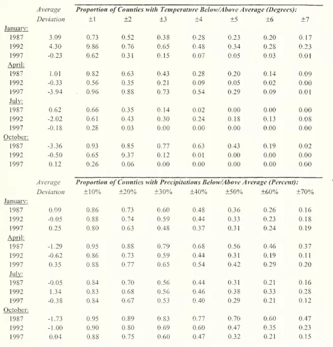
of temperaturethan precipitation.

Table 2 explores the

magnitude

ofthe deviations

between

counties' yearly weather realizations

and their longrun averages.

We

calculatethe longrun average (climate) variables asthe simpleaverage

ofall yearly county-level

measurements

from 1970 through

two

years before the

examined

year.

Each

row

reportsinformation on thedeviation

between

the relevant yearby month'srealization of temperature

or precipitation andthe correspondinglongrun average.

11

We

are indebtedto

Shawn

Bucholtzatthe

USDA

forgenerouslygeneratingthisweatherdata.

12

The

sample

is constructedto have abalanced panel ofcounties

from

1978-1997, with

none

ofthe key

variables missing.

Our

resultsarerobusttoalternativesampledefinitions. Observations from Alaska and

Hawaii

were

excluded.

13

All dollar valuesare in1997 constantdollars.

The

first

column

presents the yearly average deviation for the temperature and precipitation

variables across the 2.860 counties in our balanced panel.

The

remaining

columns

report the proportion

ofcounties with deviations at least as large as the one reported in the

column

heading. For example,

consider the January 1987 row.

The

entries indicate that

73%

ofcounties had a

mean

January 1987

temperature that

was

at least 1 degree

above

or

below

their long run average January temperature

(calculatedwiththe 1970-85 data). Analogously inOctober 1997, precipitation

was

10%

above or

below

thelongrunaverage(calculatedwithdata

from

1970-1995)in

95%

ofallcounties.

Our

baseline estimatesofthe effectofclimatechange follow theconvention intheliteratureand

assume

a uniform (across months) five degree Fahrenheit increase in temperature and eight percent

increase in precipitation associated with a doubling of atmospheric concentrations ofgreenhouse gases

(IPCC

1990;

NAS

1992).

14

It

would

be idealifameaningful fraction ofthe observationshave deviations

from long run averages as large as 5 degrees and

8%

of

mean

precipitation. Ifthis is the case, our

predicted

economic

impactswillbe identifiedfromthe data, ratherthan

by

extrapolationdueto functional

form assumptions.

In both the temperature and precipitation panels, it is clear that deviations ofthe magnitudes

predicted by the climate change

models

occurin the data. It isevidentthat forall four

months

there will

be little difficulty identifying the

8%

change in precipitation.

However

in the cases oftemperature,

deviations as large as +/- 5 degree occurless frequently, especially in July. Consequently, the effects of

thepredictedtemperaturechanges inthese

months

willbeidentifiedfrom asmall

number

ofobservations

and functional form assumptionswillplay alarger rolethan isideal.

15

III.

Econometric

Strategy

A. The

Hedonic Approach

This section describes the econometric

framework

that

we

use to assess the consequences of

globalclimatechange.

We

initially considerthehedoniccross sectional

model

thathas been predominant

in the previous literature

(MNS

1994

&

1999; Schlenker,

Hanemann,

and Fisher 2002). Equation (3)

provides a standard formulationofthismodel:

14

Mendelsohn,

Nordhaus, and

Shaw

(1994 and 1999) andSchlenker,

Hanemann,

and Fisher (2002)also

calculate the effect of global climate change based on these estimated changes in temperature and

precipitation.

15

In

some

models,

we

will include state by year fixed effects and in these specifications functional form assumptions willbe even

more

important.

(3) yet

=

Xct'P

+

2, e, f,(

W

ic)

+ E*

SM

=

a

c

+

uct,

where

yct isthevalue ofagricultural landper acre in county c in yeart.

The

tsubscript indicates that this

model

couldbeestimatedin any yearfor

which

dataisavailable.

X

ct is a vectorof observable determinants of farmland values.

A

tsubscript is included

on

the

X

vector, because itincludes

some

time-varying factors that affect land values.

W

ic represents aseries of

climate variables for county c.

We

follow

MNS

and let i indicate one ofeight climatic variables. In

particular, there are separate measures of temperature and total precipitation in January, April, July, and Octoberso there isone

month

from each quarteroftheyear.

The

appropriate functional form for each of

the climate variables is

unknown,

but inourreplication ofthehedonic approach

we

followtheconvention

in the literature and

model

the climatic variables with linear and quadratic terms.

The

last term in

equation(3)isthe stochastic error term, sct,thatis comprised ofapermanent,county-specific

component,

ctc,and an idiosyncraticshock,uct.

The

coefficient vector is the 'true' effect ofclimate

on

farmland values and its estimatesare

used to calculatethe overall effectofclimate change associatedwiththe

benchmark

5-degree Fahrenheit

increase in temperature and eight percent increase in precipitation. Since the total effect of climate

change is a linear function of the

components

ofthe 6 vector, it is straightforward to formulate and

implement

testsofthe effectsofalternativeclimatechange scenarioson agricultural land values.

We

will

reportthe standarderrors associated withthe overall estimate ofthe effect ofclimatechange.

However,

thetotal effect ofclimate

change

isa function of 16 parameter estimates

when

the climate variables are

modeled

with a quadratic, so it is not surprising that statistical significance is elusive. This issue of

samplingvariabilityhas generally been ignoredintheprevious literature.16

Consistent estimation ofthe vector 6,and consequently ofthe effect ofclimate change, requires

that

E[fi(W

ic) Ectl

X

ct]

=

_{for each climate variable}

i. This assumption will be invalid ifthere are

unmeasured permanent

(ac) and/or transitory (uct) factors that covary with the climate variables.

To

obtain reliableestimates of8,

we

collecteda

wide

range ofpotential explanatory variables including all

thesoilquality variables listed inTable 1, aswell asper capita

income and

populationdensity.17

We

also

estimate specificationsthatincludestate fixedeffects.

16

Schlenker,

Hanemann,

andFisher(2002)isanotable exception.

1

Previous research suggests that urbanicity, population density, the local price of irrigation, and air

pollution concentrations areimportant determinantsoflandvalues (Cline 1996; Plantinga,Lubowski, and

There arethree furtherissues about equation(2) thatbearnoting. First, it islikely that the error

terms are correlated

among

nearby geographical areas. For example, unobserved soil productivity is

likely tobe spatially correlated. In thiscase,the standard

OLS

formulasfor inferenceare incorrect since

the error variance is not spherical. In absence of

knowledge on

the sources and the extent ofresidual

spatial

dependence

inlandvaluedata,

we

adjustthestandarderrors for spatial

dependence

of an

unknown

form

following the approachof

Conley

(1999).

The

basicideaisthatthespatial

dependence

between two

observationswilldecline as the distance

between

the

two

observationsincreases.18

Throughout

the paper,

we

present standard errors calculated withthe Eicker-

White

formulathatallows forheteroskedasticity of

anunspecifiednature, inadditiontothose calculatedwiththe

Conley

formula.

Second, it

may

be appropriate to weight equation (3). Since the dependent variable is

county-level farmland values per acre,

we

think there are

two complementary

reasons to weight

by

the square

root of acres of farmland. First, the esiimates of the value of farmland from counties with large

agricultural operations will be

more

precisethan the estimates from counties with small operations and

theweightingcorrects forthe heteroskedasticityassociated withthe differences inprecision. Second,the

weighted

mean

ofthe dependent variable isequal tothe national value of farmland normalized

by

total

acresdevotedtoagriculture inthecountry.

MNS

estimate

models

that use the square rootsofthe percent ofthecounty in cropland

and

total

revenue from crop sales as weights, respectively.

We

also present results based on these approaches, althoughthe motivation for these weighting

schemes

is less transparent. For example, they both correct

forparticular forms ofheteroskedasticity but it is difficulttojustifythe assumptions aboutthe

variance-covariance matrix that

would

motivate these weights. Further, although these weights

emphasize

the

countiesthatare

most

importanttototalagricultural production,they do soinan unconventionalmanner.

Consequently, the weighted

means

ofthe dependent variable with these weights have a non-standard

interpretation.

Third toprobe the robustnessofthehedonic approach,

we

estimateit withdata

from

each ofthe

Census years. Ifthis

model

is specified correctly,the estimates will be unaffected

by

theyear in

which

the

model

is estimated. Ifthe estimates differ across years, this

may

be interpreted as evidencethat the

hedonic

model

ismisspecified.

Stavins2002; Schlenker,

Hanemann,

and Fisher2002;

Chay

and Greenstone 2004).

Comprehensive

data

onthe priceofirrigation andairpollutionconcentrations

were

unavailable.

8

More

precisely, the

Conley

(1999) covariance matrix estimator is obtained

by

taking a weighted average of spatial autocovariances.

The

weights are given by the product ofBartlett kernels in

two

B.

A

New

Approach

One

ofthis paper's primary points is that the cross-sectional hedonic equation is likely to be

misspecified.

As

a possible solutiontothese problems,

we

fit:

(4) yct

=

occ

+

y,

+

X

c/(3

+ S

: 6, f,(Wlct)

+

uct.

There are a

number

of important differences

between

equations (4) and (3). For starters, the equation

includes a full set of county fixed effects,

a

c.

The

appeal of including the roughly 3,000 county fixed

effects is that they absorb all unobserved county-specific time invariant determinants ofthe dependent

variable.19

The

equation also includes year indicators, y,, that control for annual differences in the

dependent variable that are

common

across counties.

As

discussed above,

we

also report results from

specifications

where

we

replace theyearfixedeffectswithstate

by

yearindicators.

The

inclusion ofthe county fixedeffects necessitates

two

substantive differences in equation (4),

relativeto(3). First, since thereis

no

temporal variation in

W

jc,itis impossibleto estimate the effect of

the long run climate averages. Consequently,

we

replace theclimate variableswith annualrealizationsof

weather,

W,

ct. Thus,theequation includesmeasures ofJanuary, April, July and October temperature and

precipitation inyeart.

We

allow fora quadratic ineach ofthesevariables.

Second, the dependent variable, yct, is

now

county-level agricultural profits, instead of land

values. This isbecause landvalues capitalize longrun characteristics ofsites and, conditional

on

county

fixedeffects, annual realizations ofweather should notaffect land values.

However,

weather does affect

farm revenues and expenditures and their difference is equal to profits.

The

association

between

the

weather variables and agricultural profits

may

be dueto changes in revenues or operating expenditures

and

we

show

separate results for each of these potential outcomes. Further,

we

use the separate

subcategoriesof farm expenditures (e.g., labor, capital, and inputs) asdependent variablestoexplore the

rangeofadaptations availableto farmers inresponsetoweathershocks.

The

validity ofany estimateoftheimpactofclimate

change

based

on

equation(4) rests crucially

on the assumption that its estimation will produce unbiased estimates ofthe 8 vector. Formally, the

consistencyof each8j requires E[fj(Wict)uct|

X

ct,

a

_c, y,]=0.

By

conditioningon thecounty and year fixed

effects, 6 is identified from county-specific deviations in weather about the county averages after

controlling for shocks

common

to all counties in a state. This variation is

presumed

tobe orthogonal to

unobserved determinants ofagricultural profits, so itprovides apotential solutiontotheomittedvariables

biasproblemsthatappeartoplaguetheestimation of equation(3).

A

shortcomingofthisapproach isthat

onethe coordinates exceeds apre-specified cutoffpoint.

Throughout

we

choosethe cutoff pointsto be 7

degreesoflatitudeandlongitude, correspondingtodistancesof about

500

miles.

the inclusion of these fixed effects is likely to

magnify

the importance of misspecification due to

measurement

error,

which

generally attenuates the estimated parameters.

IV. Results

Thissection isdividedintothree subsections.

The

firstprovides

some

suggestiveevidence

on

the

validity ofthe hedonic approach and then present results

from

this approach.

The

second subsection

presents results

from

the fittingof equation(4),

where

county-level agricultural profits arethe dependent

variableand the specification includes a full set of countyfixed effects. It also probes the robustness of

these results.

The

third andfinal subsection againfits equation(4), buthere the dependentvariables are

the separate determinants ofprofits.

The

aim

is to understand the adaptations that farmers are able to

undertake inresponsetoweathershocks.

A.Estimates ofthe

Impact of

Climate

Changes

from

the

Hedonic

Approach

As

the previous section highlighted, the hedonic approach relies

on

the assumption that the

climate variables are orthogonal to unobserved determinants of land values.

We

begin by examining whetherthese variables are orthogonal to observable predictors of farm values.

While

this is not a formal test ofthe identifying assumption, there are at least

two

reasons that it

may

seem

reasonableto

presume

that thisapproach willproduce validestimates ofthe effects ofclimate

when

theobservables arebalanced. First, consistent inferencewill not

depend

on functional form assumptions

(e.g., linear regression adjustment

when

the conditional expectations function is nonlinear) on the

relations

between

the observableconfounders

and

farm values. Second, the unobservables

may

be

more

likelytobe balanced(Altonji, Elder,and

Taber

2000).

Table

3A

shows

the association of the temperature variables with farm values and likely

determinants offarm values and

3B

does the

same

for the precipitation variables.

To

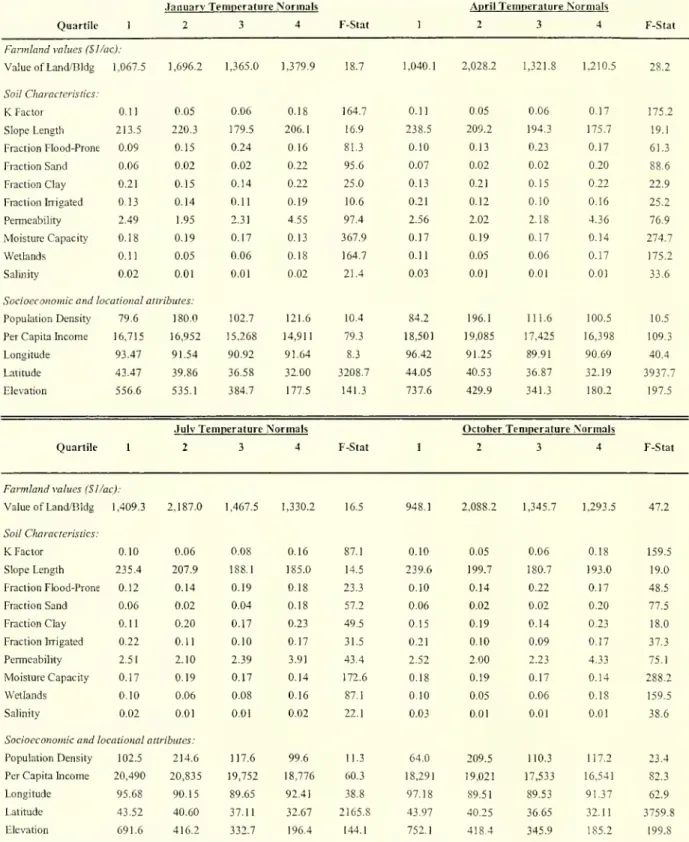
understand the

structureofthe tables, consider the upper-left cornerof Table 3A.

The

entries inthe first four

columns

arethe

means

of farmlandvalues,soil characteristics,and socioeconomic andlocational characteristics

by

quartile of the January temperature normal,

where

normal refers to the long run county average

temperature.

The means

arecalculated withdatafromthe five Censusesbut areadjustedforyeareffects.

Throughout

Tables

3A

and 3B, quartile 1 ₍₄₎ refers to counties with a climate normal in the lowest

(highest) quartile,so, forexample,quartile 1 counties forJanuary temperaturearethecoldest.

19

Interestingly, the fixed effects

model

was

first developed by

Hoch

(1958 and 1962) and

Mundlak

(1961)toaccount forunobservedheterogeneityinestimatingfarm production functions.

The

fifth

column

reports the F-statistic from atest that the

means

are equal across the quartiles.

Since thereare five observations per county, thetest statistics allowsfor county-specific

random

effects.

A

value of2.37 (3.34) indicates that the null hypothesis canbe rejected atthe

5%

(1%)

level. If climate

were randomly

assigned across counties, there

would

be very

few

significant differences.

It is immediately evident that the observable determinants of farmland values are not balanced

across thequartiles ofweathernormals. In 120 (119) ofthe 120cases,the null hypothesisofequality of

the sample

means

ofthe explanatory variables across quartiles can be rejected at the

5%

(1%)

level. In

many

cases the differences inthe

means

are large, implying thatrejectionofthenull isnot simply dueto

the sample size. For example, the fraction ofthe land that is irrigated and the population density (a

measure

ofurbanicity) in the county are

known

to be important determinants of the agricultural land

values and their

means

vary dramatically across quartiles ofthe climate variables. Overall, the entries

suggest that the conventional cross-sectional hedonic approach

may

be biased due to incorrect

specificationofthe functional

form

of observedvariables and omitted variables.

With

these results in mind, Table 4 implements the hedonic approach.

The

entries are the

predicted change in land values from the

benchmark

increases of5 degrees in temperatures

and

8%

in

precipitation from 72different specifications.

Every

specificationallows fora quadratic ineach ofthe 8

climate variables.

Each

county's predicted

change

is calculated as the

sum

ofthe partial derivatives of

farm values with respect to the relevant climate variable at the county's value ofthe climate variable

multiplied by the predicted change in climate (i.e., 5 degrees or 8%).

These

county-specific predicted

changesare then

summed

across the2,860countiesinthe

sample

and

reported inbillionsof1997 dollars.

For the year-specific estimates, the heteroskedastic-consistent (White 1980) and spatial standard errors

(Conley 1999) associated with each estimate are reported in parentheses. Forthe pooled estimates, the

standarderrorsreportedinparenthesesallowforclusteringatthecountylevel.20

The

72 sets of entries are the result of 6 different data samples, 4 specifications, and 3

assumptions about the correct weights.

The

data samples are denoted in the

row

headings. There is a

separate

sample

for each ofthe

Census

years and the sixth is the result of pooling data from the five

Censuses.

Each

ofthe foursetsof

columns

corresponds toadifferentspecification.

The

firstdoesnot adjust

for any observable determinants of farmland values.

The

second specification follows the previous

literature and adjusts for the soil characteristics in Table 2, as well as per capita

income

and population

density

and

its square.

MNS

suggest that latitude, longitude, and elevation (measured at county

centroids)

may

be importantdeterminantsofland values, so thethirdspecification addsthese variables to

20

Sincethepooledmodelshavea largernumberofobservations, thespatial standarderrorswerenot estimated

because oftheircomputationalburden.

the regression equation.21 2'

The

fourth specification adds state fixed effects.

The

exact controls are

notedinthe

rows

atthebottom ofthe table.

Within each set of columns, the

column

"[1]" entries are the result of weighting by the square

root offarmland. Recall, this

seems

like the

most

sensible assumption about the weights. In the "[2]"

and "[3]" columns, the weights are the square root ofthe percentage of each county in cropland and

aggregate valueofcroprevenueineachcounty.

We

initially focus

on

the first five rows,

where

the samples are independent.

The most

striking featureoftheentries isthetremendousvariationintheestimatedimpact ofclimatechange onagricultural

land values. For example, the estimates range

between

positive

$265

billion and minus

$422

billion,

which

are

19%

and

-30%

ofthe totalvalue oflandand structuresin this period.

An

especially unsettling

feature ofthese results is that even

when

the specification and weighting assumption are held constant,

the estimated impact can vary greatly depending on the sample. For example, the estimated impact is

roughly

$200

billion in 1978 but essentially$0 in 1997, with specification #2 andthe square root ofthe

acres of farmlandas the weight. This finding is troubling becausethere is

no

ex-antereason to believe

that the estimate from an individual year is

more

reliable than those from other years.23 Finally, it is

noteworthythat the standard errors are largest

when

the square root ofthe crop revenues is the weight,

suggestingthatthisapproachfitsthe dataleastwell.

Figure 1 graphically

summarizes

these60 estimates ofthe effectofclimatechange. This figure

plots eachofthe point estimates, along with their +/- 1 standard errorrange.

The

widevariability ofthe

estimates is evident visually and underscores the sensitivity ofthis approach to alternative assumptions

and data sources.

An

eyeball averaging technique suggests that together they indicate a modestly

negativeeffect.

Returning to Table 4, the last

row

reports the pooled results,

which

provide a

more

systematic

method

to

summarize

the estimates from each ofthe 12 combinations ofspecifications and weighting

1

This specification is identical to

MNS'

(1994) preferred specification, except that it also controls for

longitude.

The

resultsare virtually identical

when

longitudeisexcluded.

2

We

suspect that controlling for latitude is inappropriate, because it is so highly correlated with

temperature. Forinstance,Table 3

A

demonstratesthatthe F-statisticsassociatedwith thetestofequality

ofthe

means

oflatitudeacross thetemperature normalsare roughly an orderof magnitudelargerthan the

nextlargest F-statistics. This suggeststhat latitudecaptures

some

ofthe variation thatshouldbe assigned

to the temperature variables and thereby leads to misleading predictions about the impact of climate

change. Nevertheless,

we

reportthe resultsfromthis specificationforcomparability with

MNS'

analysis.

13

We

testedwhetherthe marginal effects ofthe climate variables are equal acrossthe datafrom the five

censuses

when

the specification and weighting procedure are held constant. Innearly all cases, the null

hypothesisofequalityofthemarginal effectsisrejectedbyconventional criteria.

procedures.24

The

estimated change in property values

from

the

benchmark

global

warming

scenario

ranges from -$248 billion (witha standard errorof $21 1 billion) to

$50

billion (with a standard error of

$43 billion).

The

weighted average ofthe 12 estimates is -$35 billion,

when

the weights arethe inverse

ofthe standarderrors ofthe estimates.

Thissubsection has produced

two

important findings. First, the observable determinants ofland

prices are poorly balanced across quartiles of the climate normals. Second, the hedonic approach producesestimates oftheeffectofclimatechange thatare sensitive to specification,weighting procedure, and sample and generally are statistically insignificant. Overall, the

most

plausible conclusions are that eithertheeffect iszero orthis

method

isunableto produceacredible estimate. In lightofthe importance

ofthe question, itis worthwhileto consider alternative

methods

to valuethe

economic

impact ofclimate

change.

The

remainderofthepaperdescribes theresults from ouralternativeapproach.

B.Estimates ofthe

Impact

of Climate

Change

from

Local Variation in

Weather

We

now

turn to our preferred approach that relies

on

annual fluctuations in weather about the

monthly county normals of temperature and precipitation to estimate the impact ofclimate

change on

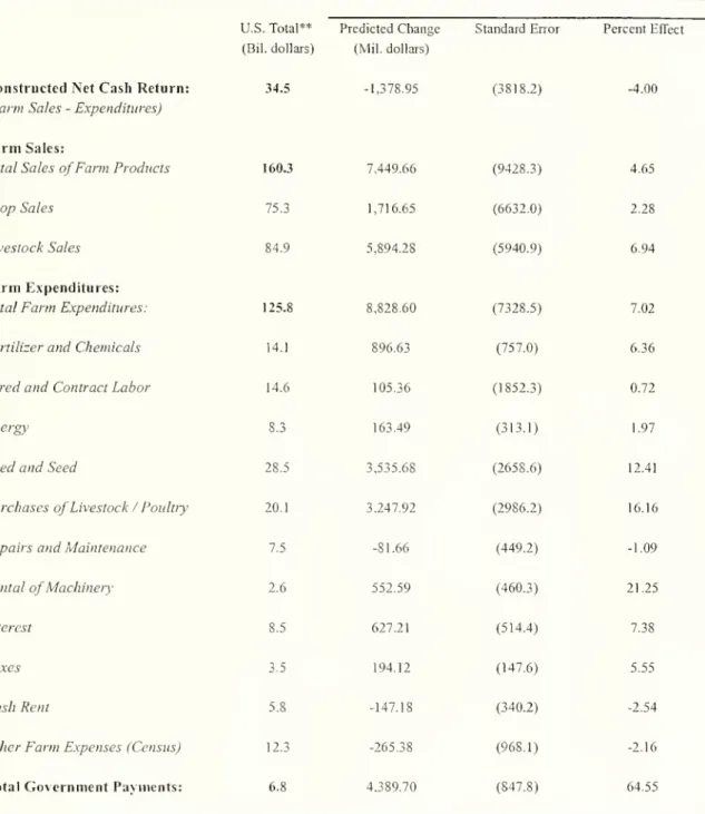
agricultural profits. Table 5 presents the results

from

the estimation of four versions of equation (4),

where

the dependent variableis county-level agriculture profits (measured in millions of 1997$) and the

weather measures are the variables ofinterest.

The

weather variables are all

modeled

with a quadratic.

The

data forthese

and

the subsequenttablesare

from

the 1987, 1992, and 1997 Censuses,since theprofit

variableisnot availableearlier in earlierCensuses.

The

specification details are notedatthe bottom ofthetable.

Each

specification includes a full

setof county fixedeffects ascontrols. In

columns

(1) and(2), the specification includes unrestrictedyear

effects and these are replaced with state

by

year effects in

columns

(3) and (4).

25

Additionally, the

columns

(2) and (4) specifications adjust for the full set of soil variables listed in Table 1, while the

columns

(1)and(3)estimatingequationsdo notinclude thesevariables.

The

first panel of the table reports the marginal effects and the heteroskedastic-consistent

standarderrors (inparentheses) of each oftheweather measures.

The

marginal effects

measure

the effect

ofa 1-degree(1 inch)

change

in

mean

monthly temperatures(precipitation) at the climate

means

on total

agricultural profits,holding constant the otherweathervariables.

The

second panel reports p-values

from

separate F-tests that the temperature variables, precipitation variables, soil variables, and county fixed

effectsare jointly equalto zero.

Inthe pooled regressions, the intercept andthe parameters

on

all covariates, except the climate ones,

The

third panelofthetable reportsthe estimatedchangein profits associatedwith the

benchmark

doublingof greenhouse gases

and

theEicker-

White and Conley

standarderrorsofthisestimate. Justas in

the hedonic approach,

we

assume

a uniform 5 degree Fahrenheit and

8%

precipitation increases. This

panel alsoreports theseparateimpacts ofthechanges intemperature andprecipitation.

When

thepointestimates aretakenliterally, itisapparentthatthe impactofauniformincrease in

temperature and precipitation will have differential effects throughout the year. Consider the marginal

effects

from

the

column

(4) specification,

which

includes the richest set ofcontrols. For example, a

5-degree increase inApril temperatures is predicted to decrease

mean

county-level agricultural profits

by

$1.35 million,

compared

to annual

mean

countyprofits of approximately $12.1 million.

The

increase in

January temperature

would

reduce agricultural profits by roughly $0.70 million, while together the

increases inJuly andOctober temperature

would

increase

mean

profits

by

$1.45 million.

The

increase in

precipitation in January

and

July is predicted to increase profits, while the October and April increase

would

decreaseprofits.26

When

these separateeffectsareadded

up

andthetotal

summed

overthe2,860

US

counties inour

sample, the net effect of the 5 degree increase in temperature and

8%

increase in precipitation is to

decrease agricultural profits

by

$1.9 billion,

which

is

5.3%

ofthe $36.0 billion in annual profits.

The

predicted change in precipitationplaya small roleinthisoverall effect, underscoringthatthetemperature

change is the potentially

more

harmful part ofclimate change for agriculture.

These

predicted changes

are a function of 16 estimated parameters, so it is not especially surprisingthat the estimated decline is

not statistically different

from

zero, regardless of whether the heteroskedastic-consistent standard errors

or larger spatial standard errors are used tojudge statistical significance. Further, separate tests cannot

reject thateither the change in temperatureor the

change

in precipitation have no impact on agricultural profits.

There are a

few

other noteworthy results. First, the marginal effects in (1) and (2) differ from

those in (3) and (4)

which

indicates that there are state-level, time-varying factors that covary with the

county-specific deviations in weather.

The

changes in the marginal effects are occasionally large, but

theytend to cancel each otherout.27 For example,the overall predicted change inprofits is -$3.5 billion

in

column

(2), but the differencewiththe-$1.9billioneffect in

column

(4)is

modest

inthecontext ofthe

25

A

controlfortotal acresof farmland isincluded inall fourspecifications, so theresults reflecttheeffect

of weatherconditional

on

total farmland.

26

Although

none

ofthe marginal effects are individually statistically significant,thejoint hypothesis that

the temperature effects are equal to zero is easily rejected. Tests ofthe precipitation marginal effects

reachidenticalconclusions.

27

For example,the October temperature marginal effect is -0.70 in the

column

(2) specification and0.22

in

column

(4), whiletheJanuary temperature marginaleffectis0.46and-0.14 inthe

same

specifications.