Dynamic weapon-target assignment problems with vulnerable C2̳ nodes

June 1988

Report LIDS - P .1786

DYNAMIC WEAPON-TARGET ASSIGNMENT

PROBLEMS WITH VULNERABLE C

2

_NODES

by

Patrick A. Hosein

James T. Walton

Mlichael Athans

Laboratory for Information and Decsision Systems

Massachusetts Institute of Technology

DYNAMIC WEAPON-TARGET ASSIGNMENT PROBLEMS

WITH VULNERABLE C

2

NODES

Patrick A. Hosein, James T. Walton and Michael Athans

Laboratory for Information and Decision Systems Massachusetts Institute of Technology

Cambridge, MA 02139

ABSTRACIT observe the outcomes of some engagements before making

further assignments). This is sometimes called a shoot-look-In this paper we present a progress report on our work on shoot strategy in the literature. In this paper we will provide the dynamic version of the Weapon to Target Assignment some results on simple cases of the dynamic problem and (WTA) problem and on the static version of the WTA problem make comparisons with the corresponding static problem. in which vulnerable C3nodes are included in the formulation. The above resource allocation problem will typically be

In the static WTA problem, weapons must be assigned to solved at a C3node and the results transmitted to the relevant targets with the objective of minimizing the total expected

number (or value) of the surviving targets. In the dynamic resources. These C3 nodes will therefore be of vital version, this allocation is done in time stages so that the importance to the defense since their destruction will in effect outcomes of previous engagements can be used in making paralyze the resources over which they have control. One future assignments. We will show that, for the simple cases approach, that can be used to increase the reliability of the studied, there is a significant cost advantage in using the system, is to replicate the C3 nodes. In this way destruction of dynamic strategy. We believe that similar results will hold for the primary C3node does not affect the defense's system since

the more general problem. its function can then be performed by one of the "backup" C3

In the static defense-asset problem with vulnerable C3 nodes. We have formulated a model which includes these nodes the offense is allowed to either attack the assets replicated nodes and will provide results on simple cases of the themselves or to first attack the command and control system, problem.

and then the assets; if the C3nodes are destroyed then the

defensive interceptors are assumed unusable. We first consider This paper is in effect a progress report of our work on simple cases where assumptions are made as to offensive and the resource allocation problem and on the survivability issue defensive states of knowledge and kill probabilities. Strategies mentioned in the previous paragraph. The models being used are then developed and optimal weapon allocations identified. are rich enough to capture the nature of the mission (e.g. These assumptions are then relaxed, and further examples defense of assets), enemy strength (number and effectiveness

demonstrate the ensuing complexity. of the enemy's weapons), defense strength (number and

effectiveness of the defense's weapons) and strategy and tactics (preferential defense, shoot-look-shoot, etc.) It should be noted that basic research studies on these topics are virtually

L INTRODUCTION non-existent.

Our long-range research objective is the quantitative study Our work is motivated by military defense problems, two of the theory of distributed C3 organizations. Our present examples of which are as follows. The first example involves research has been concentrated on certain aspects of situation the Anti-Aircraft Weapon (AAW) defense of the Naval battle

assessment and resource commitment. group or battle force platforms. The assets being defended are

aircraft carrier(s), escort warships and support ships each of Situation assessment entails the use of sensors to detect which is of some intrinsic value to the defense. The threat to and track the enemy and its weapons (i.e missiles, tanks etc.) these assets are enemy missiles launched from submarines, These sensors are usually geographically distributed so that surface ships and aircraft. These missiles may have different distributed algorithms are desirable. This problem can be damage probabilities which depend on the missile type, target formulated as a distributed hypothesis testing problem. Results type, etc. The defense's weapons are different types of AAW on this research can be found in the paper by Papastavrou and interceptors launched from Aegis and other AAW ships. The

Athans [1] in these proceedings. kill probability of these weapons may also depend on the

specific target-interceptor pair. The objective of the defense is The resource commitment problem deals with the optimal to maximize the expected surviving value of the assets. The assignment of the defense's resources against the offense's problem is to find which AAW interceptors should be assigned forces so as to minimize the damage done to the defense's to each of the enemy missiles, when should they be launched assets. If the battle is such that the defense has a single and why. This formulation allows for a preferential defense opportunity to engage the enemy then the problem can be where, in a heavy attack, it may be optimal for the defense to formulated as a static resource allocation problem. If multiple leave "low" valued assets undefended and concentrate its engagements are possible (as for example in the Strategic resources on saving the "high" valued assets.

Defense System (SDS) scenario) then better use can be made of the defense's resources by assigning them dynamically (i.e.

The second motivating example for our work is the Maximum Marginal Return algorithm, works by assigning the midcourse phase of the Strategic Defense System. In this case weapons sequentially with each weapon being assigned to the the assets are our (the defense's) Inter-Continental Ballistic target which results in the maximum marginal return in the Missile (ICBM) silos, military installations, C3 nodes, objective function.

populations centers, etc. The threat to these assets are enemy

re-entry vehicles (RV's), surrounded by decoys. The In the special case in which the kill probability is the same defense's weapons are Space-based kinetic-kill vehicles for all weapon-target pairs and all targets have the same value, (SBKKV's) and ERIS interceptors. The objective of the the optimal assignment is obtained by dividing the weapons as defense is the maximization of the expected surviving value of evenly as possible among the targets.

the assets. The problem is the determination of the optimal weapon-target assignments and the timing of the interceptor launches.

launches. 3. THE DYNAMIC WTA PROBLEM

2. THE STATIC TARGET-BASED WTA PROBLEM The battle scenario for the dynamic problem is the same as

for the static problem except that the weapon assignments are In this section we will present the static version of the done in time stages each of which consists of the following

target-based WTA problem. In this model, a number of steps:

missiles (the targets) are launched by the offense. The defense (a) Determine which targets have survived the last

has a number of interceptors (the weapons) with which to engagement,

destroy these missiles. The defense assigns a value to each of (b) Assign and fire a subset of the remaining weapons with the targets based on factors such as target type, point of the objective of minimizing the total expected value of the impact, etc. Associated with each weapon-target pair is a kill surviving targets at the end of the final stage.

probability which is the probability that the weapon will We have looked at some simple cases of this problem to gain destroy the target if it is fired at it. We will make the insight into the general problem and to help bolster our assumption that the action of a weapon on a target is intuition.

independent of all other weapons and targets. The problem

faced by the defense is the assignment of weapons to targets 3.1 The Two-Target Case with the objective of minimizing the total expected surviving

target value. In this case we will assume that there are two targets

(N=2), the kill probability is the same for all weapon-target

2.1 Mathematical Statement of the Static WTA Problem pairs, the defense has M weapons and there are K time

stages.With these assumptions we have proved the following

The following notation will be used: theorem:

N = the number of enemy targets

= the number of defense weaponrgets Theorem 3.1 Under the assumptions given above, an optimal

Vi = the number of defense weapons strategyfor the present stage can befound as follows. Let T =

Pij = probability that weaponj kills target i if shot at it rM/Ki. Solve the corresponding static problem with T

The solution will be represented by: weapons and denote the solution by {xi}where xiis the

optimal number of weapons to be assigned to target i. The

1 if weapon j is assigned to target i optimal assignment for the present stage of the dynamic

xiJ = o problem is to assign xiweapons to target i.

0 otherwise

The optimization problem can now be stated as: If we further assume that Vi=l and that M is divisible by

N M 2K then it can be shown that the optimal target leakage J(K) is

mill

J =XV

1

Jl,-

p"

(2.1) given by:

min ' = .2 V(1 1- Pi)'(.

{xij~ {0,1} } i=1 j=M

J(K) = 2K(1 -p) -2(K- 1)(1

-p)

. (3.1)

subject to:

_xx

=1 j1,. = 1,2 M Note that if K is large then the optimal leakage J(K) = 2(1-p)M

*u to J ij M ,_,,.-while the optimal leakage for the corresponding static problem

is 2(l-p)M/2. In other words, roughly half as many weapons The objective function is the total expected value of the are required for the dynamic strategy to obtain the same surviving targets while the constraint is due to the fact that expected leakage as that of the static strategy. This expresses,

each weapon can attack only one target. in a convenient form, the value of the battlespace to the

defense. 2.2 Comments on the Solution of the Static WTA Problem

In figure 1 we have plotted the ratio of the K-stage This problem has been proven, by Lloyd and leakage to the static leakage versus the kill probability p for the Witsenhausen [2], to be NP-Complete in general. This means case of two targets and 16 weapons. We have plotted the cases that polynomial time algorithms for obtaining the optimal K = 2, 4 and 8. First note that the leakage advantage of the solution do not exist. One must therefore resort to sub-optimal dynamic strategy over the static one increases with the kill

algorithms. probability. This is due to the fact that as the kill probability

increases, the information gained from the first stage In the special case in which the kill probabilities are increases. This implies that more effective use will be made of independent of the weapons, denBroeder et al. [3], have (costly) high accuracy weapons if the dynamic strategy is proposed an optimal algorithm for the problem which runs in used. Next, note that the leakage advantage of the dynamic polynomial time. This algorithm, which is usually called the strategy increases with the number of stages. This is due to the

-3-fact that the information gained increases with the number of 32 The TwoStage, N-Target Case

stages. Note, however, that most of the improvement is

obtained after only a small number of stages. In other words, In this section we will consider the two-stage dynamic

the curves rapidly converge as the number of stages increases.

This implies that, even if the number of stages is small, the singlem with N equally p (for all stages and w eapon-target single kill probability p (for all stages and weapon-target dynamic strategy offers a significant leakage advantage. pairs), and M weapons. Unlike the two target problem, we were unable to find an analytical solution to this problem for the case N>2. However, we were able to derive useful

K-stage leakage properties of the optimal solution. The first property, which

static leakage holds for the more general problem of K stages, is given as

theorem 3.2.

0.9 , Theorem 3.2 The optimal solution to the problem given

above has the property that the weapons to be used at each

0.8 stage are spread evenly among the surviving targets.

0.7 A - K-2 The above result simplifies the problem to be solved. Let

o e ' \0.8 ...K 8 us consider the two-stage problem. Let M2denote the number

of weapons used in the first stage (i.e. 2 stages to go). The

0. e _ number of weapons that will be used in the last stage will then

be M-M2. Denote the corresponding cost of the assignment, in

0.4 - which weapons are spread evenly at each stage, by J(M2). The

optimal solution can then be obtained by minimizing J(M2)

over the set

{0,1

...,M}.

o.2

If J(M2) happened to have a "convex" shape (i.e have the

0o. property that J(M₂+1) - J(M2) 2 J(M2) - J(M2-1)) then the

above minimization could be done efficiently. Unfortunately,

0 0.1 0.2 0.3 0.4 0.8 0.8 0.7 0.8 0.9 I we can show (by example) that this is not the case.

kill probability p

Let us now consider the case of K stages, N equally

Figure 1: J(K)/J(1) vs. p for the case M=16 and N=2 valued targets, a single kill probability and M weapons with

the constraint that the number of weapons is less than the number of targets. Our intuition tells us that a dynamic Figure 2 contains plots of the ratio of the two-stage allocation should not perform any better than a static leakage to the static leakage versus the kill probability p for the allocation. This is in fact the case. This result is given in the

case of two targets. We have plotted the cases for which M = following theorem.

4,8,12,16 and 20. Note that the leakage advantage of the

dynamic strategy increases with the number of weapons used. Theorem 3.3 Under the assumptions given above, a

Note also that the same leakage advantage can be obtained by dynamic allocation cannot perform any better than a static

either using a few high accuracy weapons or many low allocation. Hence it is optimal to assign all of the weapons in

accuracy weapons. thefirst stage.

The above theorem is not particularly enlightening but it allows us to concentrate on the cases in which M>N. Let us

static leakage now consider the case in which there are two stages, N targets

each of unit value, a single kill probability p and M weapons

Ko8 . S "I by A\ with M > N. As before, let M2denote the number of weapons

0 M-8 used in the first stage of a strategy.

. M-20 Theorem3.4 Under the assumptions given above, the

o-·~0.7 '- , optimal assignment has the property that M2> N.

0o.·"\ Ad - a ,\ We conjecture that the above theorem can be extended to the

\', "\case - of more than two stages.

: 0 .6\

0.4 Using the properties given above we computed the

optimal solution to the two stage dynamic problem for various

o. numbers of weapons and targets using a kill probability of p =

0\.2 --- "' 0.9. The optimal values of M₂ are given in table 1. The

0o.2 \ " number of targets varies from 1 to 10 (the columns) and the

number of weapons varies from 1 to 25.(the rows). In the

0.1 cases where the solution is non-unique we have chosen values

0ALE0 0.1 0:2 023 0:4 0 8

of

M₂which exemplify any patterns. Note that for the cases N

o o.1 0.2 0.3 0.4 0. 0. 0.7 0. 0.9 1 M < 2N-1 the optimal value of M2is N. We conjecture that

kill probability p this result holds in general but have so far failed to find a

-4-M N=I N.2 N=3 N=4 N-I N-6 N=7 N=81 N.9 N=10 ,

i

I I 1

I

1

iT

I

1F

1 2-stage leakage 2 1 2 2 21212 2 2 2 2 3 1 2 3 3 3 1 3 3 3 3 3 static leakage 4 1 2 3 4 4 41 4 4 t 4 1 5 1 2j3 4 s 5 I 5 5 5 6' i 3 [ 3 4151616I 6 616 6 7 4 4 1 3 4 i 5 6 1 7 7 7 7 7 9 5 -T5 1 516 T 819 9 0.8 1 5 5 6 4 5 7 8 I 9 10 11 6 6 6 7 5 6 7 8 9 10 12 6 6 8 6 6 I 7 8 I~~~~~~~~~~.9 10 0.7 13 7 I7 8 7 7 7 8 s 9 1I 14 7 7 8 8 10 6 8 8 9 10 0.6 15 8 8 9 9 1 6 7 8 9 10 16 8 8 9 8 10 1 2 1 7 i 8 9 10 oN-2 ,N- N 8-16 17 9 g 8 10 o 11 8 I 8 lo10 18 9g g 9 12 10 12 1 14 8 I 9 10 19 10 10 11 12 3 10 12 i 13 10 9 10 0.4 20 10 10 12 12 I 10 12 14 8 9 10 21/ 11 11 12 12 11 1 2 14 I 10 o· 22 1n1 11 12 12 10 12 14 I 1 10 i 10 23 12 12 13 13 11 12 14 16 11 11 24 12 12 14 12 2 14 12 1 4 16 18 12 0.2 2 13 1 13 15 15 15 13 1I 16 18 10 0.1

Table 1: Optimal values of M₂for N=l: 10, M=1:25, p--0.9 o0

0 5 10 16 20 26

No. of defense weapons M Figure 3 contains a plot of the ratio of the 2-stage leakage

to the static leakage versus the kill probability p with a 2:1 Figure 4: J(2)/J(1) vs. M for the case K=2 with p = 0.5 weapon to target ratio (i.e. M = 2N). We have plotted the

cases N = 2,4,6,8 and 10. Here we see that as the size of the

problem increases the leakage advantage of the dynamic model 4. DISTRIBUTION OF THE C3FUNCTION

increases. This implies that, for the problems that concern us

(i.e. large scale problems), the dynamic model has a 4.1 Introduction

significant leakage advantage over the static model.

Although distribution of C3functions is generally regarded as desirable, little quantitative insight exists as to the resulting

2-stage leakage gains. Enhanced survivability of the BM/C3 system is

static leakage typically cited as the reason for such distribution. Here we

,1~~~~~~~~ .

~~develop

a concept of vulnerability for the WTA function and

consider its effect on allocation strategies. The underlying

o.9 paradigm is the defense asset model, in which the defense

defends a collection of differently valued assets against attack. 0.8

In such an engagement the objective of the offense is to

0.7 -- N-2 minimize expected surviving defense asset value. This can be

N'-~~~~~~ ' .... 6 _{accomplished by either attacking the assets themselves or by}

0.6 - N- _N-10N first attacking the defense system, and then the assets.

o0.6 C

~

~~~~Although

~

~

\\: \\ various components of the defense system are

vulnerable we assume here that the objective is the command

0.4 and control centers, the destruction of which renders the

defensive stockpile unusable. A precursor attack increases the

0. . likelihood that the assets will be undefended and thus increases

their vulnerability, making this a potentially attractive offensive

o.2 strategy. Increased vulnerability, however, comes at the cost

of a reduction in the offensive stockpile available to attack o.1 ~assets.

0 0.1

₀

0.2 0 04 0.0. 0.7 0.8 . 1 The overall objective of the defense is to maximize

0.2 0.3 0.4 O.B 0-6 0.7 0.8 O-g

kill probability expected surviving asset value; BM/C3nodes exist and are defended only insofar as they further this. Unless some Figure 3 : J(2)/J(l) vs p for the case K=2 with M=2N redundancy is planned, a destroyed BM/C3 node causes the defensive weapons it controls to be useless. For the purposes Figure 4 contains a plot of the ratio of the 2-stage leakage of initial analysis, we assume that command and control is to the static leakage versus the number of weapons M with a centralized, and replication of function will occur at this level. kill probability p = 0.5. We have plotted the cases N = 2,4,6,8 The defense has the potential to increase expected surviving and 10. Note that the leakage advantage of the dynamic model value by allocating some portion of its stockpile to BM/C3 increases roughly exponentially with the number of weapons. defense, but in so doing reduces the number of weapons This implies that the dynamic model is significantly better even available for defending assets.

4.2 ProblemDefinition

The probability that all BM/C3nodes are destroyed, using We consider a set of Q defense assets each of value Vq to simplified probabilities, is

be defended, and a set of T identical BM/C3 nodes to do so. T at

Assets and C3 nodes are far enough apart so that a successful =

1

1 - 1 [l-p(l-r)Y']) (47)

attack on one does not affect any other. The defense can see ==l s=l

which assets or nodes are being engaged in time to intercept the attack, if desired, but cannot adaptively change weapon

assignments based on damage assessment. where a_tand ys are offensive and defensive allocations for

the precursor attack, t indexes the C3 nodes and Pc is the The defense has a stockpile of M interceptors and the offensive kill probability for C3nodes. We assume that all offense a stockpile of N missiles. Each side knows these

quantities. Interceptors are in a central stockpile, and are thus BM/C3 nodes must be destroyed to eliminate the defense. capable of defending any C3 node or asset. Initially we The offense wants to minimize U, while the defense seeks assume that all attacking missiles have the same probability of tomaximize it:

kill, p, and defending interceptors r. Thus the miss

probability for an unintercepted target (e.g. attacking missile) max min U

is (l-p), if intercepted by j defenders (l-p(l-r)i) and for i {(y,xi} fat,nq} (4.8)

such intercepted targets directed at the same asset

(l-p(l-r)i)i. Were kill probabilities dependent on weapons, targets A formal statement of the problem also includes constraints

and assets this would become (for a given asset q) reflecting stockpile size and shot integrality. The offense

Nq M allocation constraint

17[1-Pqi

1

J(1-rij)i _] (4.1)T

i=1"I j=a

,a+LNq

=N (4.9)

t=l q=1

where xij = 1 if weapon j is assigned to target i and 0

otherwise, rij = kill probability for interceptorj fired at target requires that the sum of targets directed at C3nodes and at assets sum to the offensive stockpile. The defense allocation

i, Pqi = kill probability for target i against asset q and Nq constraint indexes the set of targets aimed at asset q. The simpler

version is T at

~~~N

X~~y8 + +

~xYs

= M (4.10)

JJ

[l-p(1-r)x i'] (4.2) t=1 s=l q=l i=1 (4.2) i=l

similarly requires that defensive weapons sum to the interceptor stockpile size.

where xiis the number of defensive weapons assigned to the

i-th target. The utility function, however, is nonlinear, nonconvex and

The objective function used is nonconcave. Minimal analytical insight has been developed,

and initially we discuss small numerical examples.

U = LVu+ (1-~)Vd (4 3)

4.3 Discussion where , = probability that all C3 nodes are destroyed, Vu =

expected surviving asset value if undefended and Vd = The best way to demonstrate the complexity of strategies for such problems is to first consider simple cases. Assume expected surviving asset value if defended. The offense, then, that the defense has the last move, and also that kill seeks to minimize V and the defense to maximize it. In probabilities for targets against M/C3 nodes p and

general, probabilities for targets against BM/C3 nodes (p) and

general, interceptors against targets (r) are unity; while targets against

A No M _{assets are less than one. Assets are taken to be of equal value}

HV

T(l-rJ..)J (4.4) and hence normalized to one. The offense, then, can either

Vd 1=.di1 -q1 1i attack just the assets, or first the BM/C3nodes and then the

q7-1 i=1 j~1 assets. If the control nodes are attacked the defense will defend just one by matching each incoming missile, obviously With the above assumptions about kill probabilities, this choosing the most lightly attacked. As long as there are

reduces to interceptors left they will be so used in the first stage, for

N _{otherwise they are useless in the second. If there are any left}

for the second stage, they will similarly be employed to

Vd = 2Vqfll[lp(l-r)1 (4.5) successively defend the least attacked targets. Thus the

q=l i=l offense will attack all C3

nodes evenly, as it will also do for assets (though not necessarily at the same level for both). The expected number of surviving assets, if undefended, is Note that this is true only when C3 nodes are of equal value; the same applies to the asset attacks. The purpose of a V

~E~?·,cl-p~"·(4.6)

N. _{precursor attack, with these kill probabilities, is to deplete the}

Vu = ,! iVqGl p) q * defender's stockpile rather than to actually destroy the control

-6-In figure 6 (M=6), however, increasingly effective An example from

114],

with M=12, N=36, Q=12, p=l/3 interceptors prompts the offense to decrease its C3 attack (targets against assets), pc=r=-1, vq=l for all q and 1 radar allocation from 4 to ; expected survivors have increase d (rather than C3 node), shows that the offense minimizes significantly. This pattern continues in figure 7 for M=8, expected surviving value by exhausting the defensive stockpile with the offense switching to an asset only attack at an even in the first stage and then attacking the assets. [4] also give lower value of r. In figure 8, the offense will not attack the expected surviving values for different strategies for the same BM/C3 system even for r=.7. We conclude that more and parameters when there are 2 radars, and find that the optimal more effective defensive interceptors discourage attacks on the

offensive strategy is to ignore the C3 nodes and attack the BM/C3 system. assets with the entire stockpile. But with the unity kill

probabilities used, it can be observed that the offense will never choose a two stage attack (regardless of the value of p) if there is more than one radar. Since the offense attacks radars evenly, the defense receives a target-to-interceptor

exchange ratio equal to the number of radars, and this makes a precursor attack undesirable.

When the assumption of unity kill probabilities is relaxed, .

strategies become much more complex. Interceptors might no 7

longer be singly matched to targets, and the destruction of C3 nodes loses its binary character. The offense and defense are able only to modulate the probability that nodes and targets are destroyed. The defense last-move case becomes a two-stage allocation problem, with two different defensive objectives: BM/C3 allocation strategies seek to maximize the probability of

at least one node surviving, while asset defense tries to maximize the expected surviving value.

In [4]'s example the offense would not attack the BM/C3 system if there were more than one node. Another example shows that this no longer need hold when weapons are imperfect. For the case of Q=4, N=12, p=.9 (both assets

and C3nodes) and r ranging from .7 to 1.0, figures 5-8 show e

optimal strategies for M=4, 6, 8 and 10. Note that the optimal strategies were obtained by an intelligent enumeration:

against candidate offensive strategies the defense employs that Figure 6: 9, P= 9,Q 4,N 12, M = 6

allocation which maximizes U; the offense then selects the strategy corresponding to the minima of these maxima. Only by simplifications regarding p, r and the v_i is such an enumeration feasible. In figure 5 (M=4) the offense allocates 4 of its 12 weapons to attack the C3nodes when r is low, but increases to 8 when r is high; this corresponds to defensive allocations of at first 2 and then 3 interceptors in defense of the

C3nodes. Not surprisingly, the number of expected survivors .L

is quite low.

J

I

.0 Figure 7: c = 9, Pa = 9, Q 4, N 12, M 8

QP[

-7-C_

al

o,) ." ' 'as"g0az f;

Figure 8: PC =.9, P =.9, Q =4,N= 12, M = 10

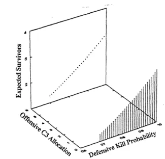
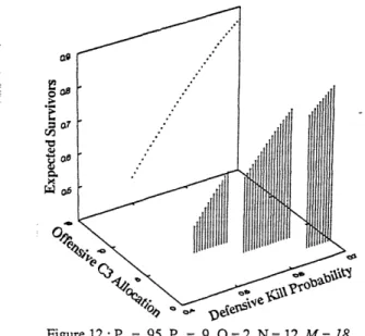
In figures 9-12 we present the results when the C3nodes 'e°a

are softer targets than the assets: Pc = .95 and Pa (assets) =

.9; other parameters are Q=2, N=12 and r from .5 to .7. When M=12 (figure 9) the offense attacks the C3nodes with

6 weapons for all values of r. When the defensive stockpile Figure 10: P = .95, Pa= 9, Q=2, N 12,M 14

increases to 14, the C3attack level drops to 4 only for r close to 1.0 (figure 10). If increased to 16 or 18 (figures 11 and 12), however, the offensive C3allocation drops to as low as 2 for high r, and then switches to 4 and then 6 as r drops. It can be seen that softer C3nodes encourage attack, even for relatively large defensive stockpiles.

ar;

~

~ ~

~

~

~

~

~r'E

=oe

Figure 9: PC = .95, Pa = .9, Q =2,

N

= 12,

M

= 12

-8-Os

a4 .,..

Figure 12: PC = .95, Pa = 9, Q= 2, N= 12,M= 18 e

Figure 13 shows the gain that replication of the command and control function provides. The ratio of the payoff for 2 C3 nodes to that of 1 C3node is plotted against values of r that range from .70 to 1.00 and for defensive stockpiles of 4, 8 and 12.

Payoff Ratio for Defense with 2 C3 Nodes: 1 C3 Node Figure 14: Pc=.9, P,=.9, Q=4, N=12, M=12, 1 C3 Node

+11.0000 . .oM-4 +8.500 / Offesive Stockpile 12 i-8 0 +3ZOOO ! +1.0000

!

A

.

0.70 0.77 0.85 0.92 1.00 . Defie MUlProility (r) . Figure 13

For small M (4), the gain is quite marked: it climbs from 2

7 to over 10. The plateau occurs at the point at which the offense switches from 2 to 4 and the defense from 2 to 3 weapons for the 2 C3node case. When M=8 the gain at first drops and then rises for increasing r, with the minima occurring where strategies for the one C3 node case change. Strategies remain the same for all values of r when M=12, and the gain decreases monotonically - equalling one when r

equals one. This is to be expected, since when the defense has ..

12 perfect weapons, it doesn't matter whether there are 1 or 2 i .

C3 nodes: all of the offense's weapons will be successfully intercepted. Figures 14 and 15 detail the strategies that lead to

this result, both one and two C3 nodes resulting in the same ° 6f. Defex

number of expected survivors when r=l, but with two C3 nodes being more effective for lower values of r.

-9-5. CONCLUSIONS

The introduction of feedback, i.e. optimal "shoot-look-shoot-look-shoot-..." strategies, can significantly improve defense effectiveness. Some extensions to the present model, which we plan to consider, include stage-dependent target values and kill probabilities, as well as consideration of the dynamic version of the asset-defense problem. Unfortunately, this will mean dealing with substantially increased complexity. In completing the study of the impact of vulnerable C3 nodes, a limited domain of control for each node will be introduced. This begins to consider the effect that a distributed organizational structure has on the implementation of WTA strategies, and raises such questions as how many BM/C3 nodes and of what type there should be. The issue of differing values for both C3nodes and assets must be addressed, since valuation will better enable us to quantify performance, and evaluate the tradeoffs that occur as distribution increases.

ACKNOWLEDGEMENT

This research was supported by the Joint Directors of Laboratories (JDL), Basic Research Group on C3, under contract with the Office of Naval Research, ONR/N00014-85-K-0782.

REFERENCES

1. Papastavrou, J. and Athans, M., "Optimum Configuration for Distributed Teams of Two Decision-Makers",

Proceedings of the 1988 Command and Control Research Symposium, Monterey, California, June 1988.

2. Lloyd, S.P. and Witsenhausen, H.S., "Weapons Allocation is NP-Complete", Proceedings of 1986 Summer

Conference on Simulation, Reno, Nevada, July 1986. 3. denBroeder, G.G., Ellison, R.E. and Emerling, L., "On

Optimum Target Assignments", Operations Research, Vol.7, pp. 322-326, 1959.

4. Eckler, A.R. and Burr, S.A., Mathematical Models of Target Coverage and Missile Allocation, Military Operations Research Society, Alexandria, Virginia, 1972.