Dynamically motivated spectroscopy of small polyatomic molecules

Texte intégral

(1)Dynamically Motivated Spectroscopy of Small Polyatomic Molecules by. G. Barratt Park S.B., Davidson College (2006) Submitted to the Department of Chemistry in partial fulfillment of the requirements for the degree of Doctor of Philosophy at the MASSACHUSETTS INSTITUTE OF TECHNOLOGY February 2015 c Massachusetts Institute of Technology 2015. All rights reserved. ○. Author . . . . . . . . . . . . . . . . . . . . . . . . . . . . . . . . . . . . . . . . . . . . . . . . . . . . . . . . . . . . . . . . Department of Chemistry January 8, 2015. Certified by . . . . . . . . . . . . . . . . . . . . . . . . . . . . . . . . . . . . . . . . . . . . . . . . . . . . . . . . . . . . Robert W. Field Haslam and Dewey Professor of Chemistry Thesis Supervisor. Accepted by . . . . . . . . . . . . . . . . . . . . . . . . . . . . . . . . . . . . . . . . . . . . . . . . . . . . . . . . . . . Robert W. Field Chairman, Departmental Committee on Graduate Students.

(2) 2.

(3) Dynamically Motivated Spectroscopy of Small Polyatomic Molecules by G. Barratt Park Submitted to the Department of Chemistry on January 8, 2015, in partial fulfillment of the requirements for the degree of Doctor of Philosophy. Abstract Molecular vibrational dynamics far from equilibrium, or in the vicinity of saddle points, are of utmost importance in chemistry. However, most of the standard models used by chemists only perform well near local minima in the potential energy surface. Several spectroscopic techniques are developed and applied to the study of molecules in excited states, including chirped-pulse millimeter wave spectroscopy and adaptations of millimeter-wave optical double resonance. Models for Franck-Condon factors in the linear-to-bent S1 –S0 transition of acetylene elucidate the dynamics of bright states observed in the fluorescence spectrum and provide insight for the design of spectroscopic schemes for accessing barrier-proximal vibrational levels. IR-UV double resonance spectroscopy enables characterization of the source of staggering in the ˜ state of SO2 , which arises due to vibronic antisymmetric stretch progression of the C interactions that lead to non-equivalent equilibrium SO bond lengths. Thesis Supervisor: Robert W. Field Title: Haslam and Dewey Professor of Chemistry. 3.

(4) 4.

(5) Acknowledgments First, I would like to thank my thesis advisor, Bob Field. Bob is an incredibly supportive and generous leader among his students and colleagues. Bob has infected me with his love of developing profound understanding of “simple” things. He is uninterested in collecting line lists and spectroscopic constants of important molecules for the sake of collecting line lists and spectroscopic constants of important molecules. Instead, Bob inspires his students and his colleagues to seek the narrative behind the spectrum, and always to approach high-resolution spectroscopy from the perspective of dynamics. I am humbled to receive Bob’s encouragement and support, and I could not be prouder than to be a part of Bob’s legacy. During my (somewhat lengthy) Ph.D., I have had a wide range of colleagues and collaborators from near and far—it would be impossible to mention them all in this brief section. I would like to thank Adam Steeves and Hans Bechtel for showing me the singlet project ropes. Wilton Virgo, Jeff Kay, Vladimir Petrovic, and Bryan Wong were also very supportive of me during my early years in the Field lab. I will never forget Jessica Lam, who showed everyone always the merit of taking the bull by the horns, whatever the bull may be. Yan Zhou, Tony Colombo, and Josh Middaugh overlapped with me for much of my graduate career. Yan, in particular, impresses me with his intelligence, diligence, and graciousness. David Grimes has been a terrific colleague as well, and Tim Barnum, an impressive new student, must be commended for promoting gregariousness and cohesion within the research group. I had substantially beneficial collaborations with Kirill Prozument and Josh Baraban, which are still continuing, and I hope will be fruitful for years to come. Bryan Changala was a particularly advanced UROP from whom I also learned a great deal. Towards the end of my graduate career, I collaborated substantially with JJ Jiang and Carrie Womack, both extremely talented scientists. JJ did a substantial amount of collaboration on the SO2 IR-UV double resonance project reported in this thesis. The reader should expect great work to come from him. The SO2 project was started as a collaboration with Andrew Whitehill of the Shuhei Ono group. Although 5.

(6) I don’t think my work ended up directly addressing their research interests, which are on anomalous sulfur isotope fractionation in pre-Cambrian rocks, he introduced me to an electronic state that I found very interesting and became the focus of a very fruitful project. I would like to thank John Stanton in advance for a collaboration ˜ state of SO2 . Catherine that we have recently started on vibronic coupling in the C Saladrigas and Peter Richter also contributed to the project. I am indebted to Brooks Pate and his research group—particularly Justin Neill— for teaching me the ropes of chirped-pulse microwave and millimeter-wave spectroscopy as a second year graduate student. They are both extremely generous colleagues. I am grateful to Arthur Suits for his support, and for inviting me to participate on his group’s project to introduce chirped-pulse Fourier transform microwave spectroscopy to the world of kinetics. Key players in this project include Chamara Abeysekera, James Oldham, Lindsay Zack, Baptiste Joalland, and Ian Sims. I am grateful to Hua Guo for valuable discussions on both acetylene and SO2 , and Georg Melau for stimulating discussions on spectroscopy of isomerizing systems (and German lessons!). I would like to thank Matt Nava, Kit Cummins, Celina Bermudez, and Bryan Lynch for involving me in very interesting microwave experiments on unusual conformations of molecules generated from intelligently designed precursors. I hope the kinks get sorted out in the near future, because from the hands of such insightful researchers, beautiful results will be no surprise. John Muenter, Anthony Merer, and Steve Coy have been very supportive of my work. All three are extremely knowledgeable in the field of molecular spectroscopy and I have learned a great deal from discussions with them. I would also like to mention my advisor at Davidson College, Merle Schuh, who first introduced me to dynamics and spectroscopy, and my sister, Margaret Park, who inspires me as a scientist. When I arrived at MIT, I was surprised to be presented with a nametag that said “Barratt Park.” At every other school I visited, I got a nametag that said “George,” which resulted in a lot of awkward conversations explaining that I don’t go by George. The credit belongs to Susan Brighton, whose attention to personal detail always made me feel welcomed. Brooke Podgurski was also very supportive of 6.

(7) the graduate students during my first year. Peter Guinta is an extremely competent administrator who goes above the call of duty to support our research group. I would like to thank Claudia in Cafe 4 for brightening each day as I purchase coffee. (“You’re still a student?”) I am grateful to Bob for allowing me to continue to pursue my interest in classical music during my graduate school career. As with my scientific collaborators, I have far too many musical collaborators to name. I am grateful to Adam Boyles, Keeril Makan, Elena Ruehr, and Donald Wilkinson for their mentorship. As a composer, I would like to thank Dustin Damonte and Roderick Phipps-Kettlewell for recording my song cycle, Krista Buckland Reisner and her colleagues for playing my string quartet, and MITSO for playing my suite. I am indebted to Gil Rose for giving me the opportunity to perform with Opera Boston, Boston Modern Opera Project, and Odyssey Opera. I am grateful to Lidiya Yankovskaya for inviting me to perform in two world-premiere operas. Thank you to Jess Rucinski for her work at St. John the Evangelist Church in Boston, and to the MIT G&S Players for allowing me quite by accident to become a conductor. I would like to thank Ethan A. Klein, Senior Field Group UROP, for entrusting me to serve as his Executive Administrative Assistant.. 7.

(8) 8.

(9) This doctoral thesis has been examined by a Committee of the Department of Chemistry as follows:. Professor Keith A. Nelson. . . . . . . . . . . . . . . . . . . . . . . . . . . . . . . . . . . . . . . . . . . . . . Chairman, Thesis Committee Professor of Chemistry. Professor Robert W. Field . . . . . . . . . . . . . . . . . . . . . . . . . . . . . . . . . . . . . . . . . . . . . Thesis Supervisor Haslam and Dewey Professor of Chemistry. Professor Moungi G. Bawendi . . . . . . . . . . . . . . . . . . . . . . . . . . . . . . . . . . . . . . . . . . Member, Thesis Committee Lester Wolfe Professor of Chemistry.

(10) 10.

(11) Contents 1 Design and evaluation of a pulsed-jet chirped-pulse millimeter-wave spectrometer for the 70–102 GHz region. 25. 1.1. Introduction . . . . . . . . . . . . . . . . . . . . . . . . . . . . . . . .. 26. 1.2. Spectrometer Design . . . . . . . . . . . . . . . . . . . . . . . . . . .. 28. 1.3. Power Limitation . . . . . . . . . . . . . . . . . . . . . . . . . . . . .. 29. 1.3.1. Measurement of Effective Power . . . . . . . . . . . . . . . . .. 29. 1.3.2. Power Requirements for Broadband Chirped Pulses . . . . . .. 32. 1.4. Shorter Dephasing times . . . . . . . . . . . . . . . . . . . . . . . . .. 35. 1.5. Phase Stability . . . . . . . . . . . . . . . . . . . . . . . . . . . . . .. 37. 1.6. Evaluation . . . . . . . . . . . . . . . . . . . . . . . . . . . . . . . . .. 40. 1.6.1. Spectroscopy of Ground States. . . . . . . . . . . . . . . . . .. 40. 1.6.2. Spectroscopy of Laser-Excited States . . . . . . . . . . . . . .. 44. 1.7. Instrument Noise Floor . . . . . . . . . . . . . . . . . . . . . . . . . .. 46. 1.8. Future Work . . . . . . . . . . . . . . . . . . . . . . . . . . . . . . . .. 47. 1.9. Acknowledgments . . . . . . . . . . . . . . . . . . . . . . . . . . . . .. 47. 1.10 Appendix: Part List . . . . . . . . . . . . . . . . . . . . . . . . . . .. 47. 2 Edge effects in chirped-pulse Fourier transform microwave spectra 49 2.1. Introduction . . . . . . . . . . . . . . . . . . . . . . . . . . . . . . . .. 49. 2.2. Polarization from a linearly chirped pulse in the weak coupling limit .. 51. 2.3. Limiting behavior of the polarization response with respect to pulse duration . . . . . . . . . . . . . . . . . . . . . . . . . . . . . . . . . .. 55. 2.3.1. 56. Long pulse limit . . . . . . . . . . . . . . . . . . . . . . . . . . 11.

(12) 2.3.2. Short pulse limit . . . . . . . . . . . . . . . . . . . . . . . . .. 56. 2.4. Conclusions . . . . . . . . . . . . . . . . . . . . . . . . . . . . . . . .. 60. 2.5. Acknowledgements . . . . . . . . . . . . . . . . . . . . . . . . . . . .. 60. ˜ 1 Au — 3 Full Dimensional Franck-Condon Factors for the Acetylene A ˜ 1 Σ+ X g Transition. I. Method for Calculating Polyatomic Linear— Bent Vibrational Intensity Factors and Evaluation of Calculated Intensities for the 𝑔𝑒𝑟𝑎𝑑𝑒 Vibrational Modes in Acetylene. 61. 3.1. Introduction . . . . . . . . . . . . . . . . . . . . . . . . . . . . . . . .. 62. 3.2. Methodology for the calculations . . . . . . . . . . . . . . . . . . . .. 65. 3.2.1. Vibrational Intensity Factors: Dependence of the electronic transition dipole moment on nuclear coordinates . . . . . . . .. 3.2.2. 3.3. Nuclear-coordinate dependence of the electronic transition dipole moment in the diabatic picture . . . . . . . . . . . . . .. 68. 3.2.3. Coordinate transformation . . . . . . . . . . . . . . . . . . . .. 70. 3.2.4. Coordinate transformation for bent—linear transitions . . . .. 79. 3.2.5. Method of Generating Functions . . . . . . . . . . . . . . . . .. 82. ˜ X ˜ Calculation of Coordinate Transformation Parameters for the A— System of Acetylene. 3.4. 65. . . . . . . . . . . . . . . . . . . . . . . . . . . .. 91. Evaluation of Calculated FC intensities for the gerade modes . . . . .. 97. 3.4.1. 𝑣3′ ← 0 Progession . . . . . . . . . . . . . . . . . . . . . . . . .. 97. 3.4.2. ˜ 𝑗 3𝑘 ) . . . . . . . . . . . . . . . . . . . . . . 100 Emission from A(2. 3.5. Conclusions . . . . . . . . . . . . . . . . . . . . . . . . . . . . . . . . 102. 3.6. Acknowledgements . . . . . . . . . . . . . . . . . . . . . . . . . . . . 104. ˜ 1 Au — 4 Full Dimensional Franck-Condon Factors for the Acetylene A ˜ 1 Σ+ X g Transition. II. Vibrational Overlap Factors for Levels Involving Excitation in 𝑢𝑛𝑔𝑒𝑟𝑎𝑑𝑒 Modes. 105. 4.1. Introduction . . . . . . . . . . . . . . . . . . . . . . . . . . . . . . . . 106. 4.2. ˜ X ˜ system . . . . . 108 Polyad structure and bending dynamics in the A— 4.2.1. ˜ X-state polyad structure . . . . . . . . . . . . . . . . . . . . . 109 12.

(13) 4.2.2 4.3. ˜ state . . . . . . . . . . . . . . . . . . 110 Bending modes of the A. ˜ 𝑚 61 ) . . . . . . . . . . . . . . . . . . 110 Dispersed Fluorescence from A(3 4.3.1. +1 −1 + ˜ 𝑚 61 ) → X(0,𝑣 ˜ The A(3 2 , 0, 𝑣4 , 1 )Σ𝑢 Progressions . . . . . . 110. 4.3.2. ˜ Multiple Zero-Order Bright States in Spectra from A-state 3𝑚 61 111. 4.4. Propensities in IR-UV fluorescence . . . . . . . . . . . . . . . . . . . 115. 4.5. ˜ Emission from levels of gerade B𝑛 polyads to bending levels of the X state . . . . . . . . . . . . . . . . . . . . . . . . . . . . . . . . . . . . 118 4.5.1. ˜ Fluorescence intensities and phases for transitions into X-state pure bending polyads in the normal mode basis . . . . . . . . 119. 4.5.2. ˜ intrapolyad pure bend intensities to Transformation of X-state the local mode basis . . . . . . . . . . . . . . . . . . . . . . . 124. 4.6. Conclusions . . . . . . . . . . . . . . . . . . . . . . . . . . . . . . . . 134. 4.7. Acknowledgements . . . . . . . . . . . . . . . . . . . . . . . . . . . . 135. 5 A simplified Cartesian basis model for intrapolyad emission intensities in the bent-to-linear electronic transition of acetylene. 137. 5.1. Introduction . . . . . . . . . . . . . . . . . . . . . . . . . . . . . . . . 138. 5.2. ˜ X ˜ system . . . . . 140 Polyad structure and bending dynamics in the A—. 5.3. Franck-Condon propensity rules in the Cartesian basis . . . . . . . . 141. 5.4. Corrections for anharmonic interactions . . . . . . . . . . . . . . . . . 146. 5.5. Comparison of measured emission intensity patterns with the Cartesian bright state model . . . . . . . . . . . . . . . . . . . . . . . . . . . . 148. 5.6. Analogy to nonlinear molecular systems . . . . . . . . . . . . . . . . . 152. 5.7. Discussion and Conclusions . . . . . . . . . . . . . . . . . . . . . . . 154. 5.8. Acknowledgements . . . . . . . . . . . . . . . . . . . . . . . . . . . . 158. 6 Millimeter-wave optical double resonance schemes for rapid assign˜ 1 B2 state of ment of perturbed spectra, with applications to the C SO2. 159. 6.1. Introduction . . . . . . . . . . . . . . . . . . . . . . . . . . . . . . . . 160. 6.2. Experimental details . . . . . . . . . . . . . . . . . . . . . . . . . . . 162 13.

(14) 6.2.1. Millimeter-wave optical double resonance configuration . . . . 162. 6.2.2. Available schemes for millimeter-wave optical double resonance 162. 6.2.3. Implementation of millimeter-wave optical double resonance schemes . . . . . . . . . . . . . . . . . . . . . . . . . . . . . . 169. 6.3. Results . . . . . . . . . . . . . . . . . . . . . . . . . . . . . . . . . . . 171 6.3.1. ˜ Perturbations in the C(1,3,2) level . . . . . . . . . . . . . . . . 171. 6.3.2. The 46816 cm−1 level . . . . . . . . . . . . . . . . . . . . . . . 179. 6.3.3. The 47569 and 47616 cm−1 levels . . . . . . . . . . . . . . . . 180. 6.4. Discussion . . . . . . . . . . . . . . . . . . . . . . . . . . . . . . . . . 184. 6.5. Conclusions and Future Work . . . . . . . . . . . . . . . . . . . . . . 186. 6.6. Acknowledgments . . . . . . . . . . . . . . . . . . . . . . . . . . . . . 187. 7 Direct observation of the low-lying b2 symmetry vibrational levels of ˜ 1 B2 state of SO2 by IR-UV double resonance: Characterization the C of the asymmetry staggering and the origin of unequal bond lengths189 7.1. Introduction . . . . . . . . . . . . . . . . . . . . . . . . . . . . . . . . 190. 7.2. Selection rules . . . . . . . . . . . . . . . . . . . . . . . . . . . . . . . 191. 7.3. Experimental . . . . . . . . . . . . . . . . . . . . . . . . . . . . . . . 193. 7.4. 7.3.1. Strategies for observing the b2 levels . . . . . . . . . . . . . . 193. 7.3.2. Experimental details . . . . . . . . . . . . . . . . . . . . . . . 194. Rotational structure and Coriolis interactions . . . . . . . . . . . . . 196 7.4.1. The (0,0,1) level . . . . . . . . . . . . . . . . . . . . . . . . . . 198. 7.4.2. The (0,1,1) and (0,0,2) levels . . . . . . . . . . . . . . . . . . . 198. 7.4.3. The (0,0,3), (0,1,2), (0,2,1), and (1,0,0) levels . . . . . . . . . 203. 7.4.4. The (0,0,4), (0,1,3), (1,0,1), (0,2,2), and (0,3,1) levels . . . . . 207. 7.4.5. The (0,0,5) level . . . . . . . . . . . . . . . . . . . . . . . . . . 212. 7.4.6. Summary of rotational parameters derived in this work . . . . 214. 7.5. Vibrational level structure . . . . . . . . . . . . . . . . . . . . . . . . 218. 7.6. Discussion . . . . . . . . . . . . . . . . . . . . . . . . . . . . . . . . . 221 7.6.1. ˜ state with 21 A1 . . . . . . . . . . . . . . . 221 Interaction of the C 14.

(15) 7.6.2. Evidence for increased effective barrier height along the approach to conical intersection . . . . . . . . . . . . . . . . . . 222. 7.7. Conclusions . . . . . . . . . . . . . . . . . . . . . . . . . . . . . . . . 225. 7.8. Acknowledgments . . . . . . . . . . . . . . . . . . . . . . . . . . . . . 226. A Tabulation of calculated vibrational overlap integrals from gerade ˜ state to pure bending polyad levels of the X ˜ B𝑛 polyads of the A state of acetylene. 227. B Response of a two-level system to a slowly varying excitation pulse231 B.0.1 Time dependence of the coherence . . . . . . . . . . . . . . . . 232 B.0.2 Time dependence of the macroscopic polarization . . . . . . . 233 C Electric field intensity of a free induction decay excited by a chirped pulse. 235. D Signal scaling for a thermally equilibrated molecular sample excited by a chirped excitation pulse. 237. E Term values assigned from the mmODR spectra of Chapter 6. 239. ˜ state of SO2 observed by IR-UV double resoF Term values of the C nance. 241. 15.

(16) 16.

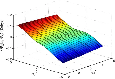
(17) List of Figures 1-1 Chirped-pulse millimeter-wave spectrometer design . . . . . . . . . .. 29. 1-2 Evaluation of the millimeter wave excitation pulse strength . . . . . .. 31. 1-3 Achievable polarization in the CPmmW spectrometer . . . . . . . . .. 33. 1-4 Comparison between perpendicular and coaxial propagation of the molecular beam and millimeter-wave pulse . . . . . . . . . . . . . . .. 36. 1-5 High-resolution CPmmW spectrum of the acetonitrile 𝐽 = 5 ← 4, 𝐾 = 0 transition with resolved. 14. N quadrupole moment hyperfine structure.. 1-6 Broadband spectrum of the photolysis products of acrylonitrile . . . .. 38 41. 1-7 Comparison of the CPmmW spectrometer performance with that of a scanned absorption spectrometer . . . . . . . . . . . . . . . . . . . .. 42. 1-8 Millimeter-wave optical double resonance spectroscopy on SO2 . . . .. 44. 1-9 Optical-millimeter wave double resonance on the excited e 3 Σ− (𝜈 = 2) state of CS . . . . . . . . . . . . . . . . . . . . . . . . . . . . . . . . .. 45. 2-1 Evolution of the response function to a chirped excitation pulse as a function of pulse duration . . . . . . . . . . . . . . . . . . . . . . . .. 55. 2-2 Pressure broadening in the 𝐽 = 6–5 transition of OCS and signal loss due to dephasing during the excitation pulse . . . . . . . . . . . . . .. 59. 3-1 The ⟨ΨA˜ |𝜇𝑐 |ΨX˜ ⟩ transition moment of acetylene, plotted as a function of 𝑞2′′ and 𝑞4′′ . . . . . . . . . . . . . . . . . . . . . . . . . . . . . . . .. 68. 3-2 Rectilinear and curvilinear internal coordinates in acetylene . . . . . .. 76. 3-3 Labeling of the acetylene nuclei and the orientation of the principal inertial axis system . . . . . . . . . . . . . . . . . . . . . . . . . . . . 17. 93.

(18) 3-4 Experimentally observed and calculated oscillator strengths for the ˜ ←X ˜ system of acetylene . . . . . . . . . 𝑣3′ ← 0 progression for the A. 99. 3-5 The magnitude of the vibrational intensity factor for the vibrationless 0–0 transition as a function of the displacement in the trans-bending ˜ and X ˜ states of mode 𝛿3′ between the equilibrium geometries of the A acetylene . . . . . . . . . . . . . . . . . . . . . . . . . . . . . . . . . . 100 3-6 Relative emission intensities for a selection of (2𝑗𝑚 V𝑘𝑛 ) vibrational tran˜ →X ˜ transition . . . . . . . . . . . . . . . . 103 sitions of the acetylene A ˜ 𝑚 61 )(b𝑢 ) to zero-order bright states 4-1 Relative emission intensities for A(3 ˜ 𝑣2 , 0, 𝑣4+1 , 1−1 )Σ+ of acetylene . . . . . . . . . . . . . . . . . . . . 112 X(0, 𝑢 4-2 Calculated emission intensities from zero-order members of low-lying B𝑛 polyads of S1 acetylene to pure bending polyads of S0 . . . . . . . 125 4-3 Calculated vibrational intensity for emission from a𝑔 members of B𝑛 ˜ ˜ state polyads of A-state acetylene to pure bending polyads of the X with Σ+ 𝑔 symmetry, illustrating access to the extreme counter rotator of each polyad . . . . . . . . . . . . . . . . . . . . . . . . . . . . . . . 129 4-4 Calculated vibrational intensity for emission from a𝑔 members of B𝑛 ˜ polyads of A-state acetylene to the extreme local bender zero-order + ˜ state, (|𝑁𝐵0 , 00 ⟩𝑔+ 𝐿 ), of each Σ𝑔 pure bending polyad of the X state . . 130. ˜ state of acety5-1 Emission spectra from levels of the 32 B2 polyad of the A lene into the {𝑁𝑠 , 𝑁res } = {0, 10} pure bending polyad set. . . . . . . 143. ˜ 5-2 Overlap of the zero-order Cartesian bright states of X-state acetylene, ˜ state, with the 𝑙 = 0, 2 zeroaccessed from 62 and 42 levels of the A order polar 2DHO basis states . . . . . . . . . . . . . . . . . . . . . . 146 5-3 High-resolution DF spectra obtained from the 32 61 and 33 61 levels ˜ of A-state acetylene into a representative collection of pure-bend and ˜ state . . . . . . . . . . . . . . . . . 148 stretch-bend polyad sets of the X 5-4 High-resolution DF spectra obtained from the 32 61 and 33 61 levels of ˜ ˜ state151 A-state acetylene into the {𝑁𝑠 , 𝑁res } = {1, 11} polyad set of the X 18.

(19) ′′ ′ ′ 5-5 The 𝜈11 (e) and the 𝜈14 (b3𝑢 ) and 𝜈15 (b2𝑢 ) vibrational modes of allene. in its 1 A1 ground state and planar D2h 1 A𝑔 excited state, respectively. 155. 6-1 Schematic drawing of the experimental configuration used for the mmODR experiments . . . . . . . . . . . . . . . . . . . . . . . . . . . 163 6-2 Schematic comparison of three FID-detected MODR schemes . . . . . 165 6-3 The coherence-converted population transfer window function . . . . 168 6-4 Pulse sequence schematics for multiplexed mmODR spectroscopy . . 172 6-5 Sample mmODR spectra obtained using a millimeter-wave implementation of the coherence converted population transfer scheme . . . . . 173 ˜ 3, 2) level 6-6 Reduced term value plot for the region surrounding the C(1, of SO2 . . . . . . . . . . . . . . . . . . . . . . . . . . . . . . . . . . . 175 ˜ 3, 2) ← X(0, ˜ 0, 0) 6-7 Relative offset in the frequency calibration of the C(1, transition in SO2 between our work and that of Yamanouchi et al., J. Mol. Struct. 352/353, 541 . . . . . . . . . . . . . . . . . . . . . . . . 178 6-8 Splitting in both the q R1 (6) and q P1 (8) transition to the 𝐽𝐾𝑎 𝐾𝑐 = 716 ˜ 3, 2) level of SO2 level of C(1,. . . . . . . . . . . . . . . . . . . . . . . 179. ˜ 6-9 Reduced term value plot for the perturbed 46816 cm−1 level of the C state of SO2 . . . . . . . . . . . . . . . . . . . . . . . . . . . . . . . . 180 6-10 Multiplexed mmODR spectrum of the 47569 cm−1 vibrational level of ˜ state of SO2 . . . . . . . . . . . . . . . . . . . . . . . . . . . . 182 the C 6-11 Multiplexed mmODR spectrum of the 47616 cm−1 vibrational level of ˜ state of SO2 . . . . . . . . . . . . . . . . . . . . . . . . . . . . 183 the C 6-12 Reduced term value plot for the 47616 cm−1 and 47569 cm−1 levels of ˜ state of SO2 . . . . . . . . . . . . . . . . . . . . . . . . . . . . 185 the C ˜ 0, 1) ← X(1, ˜ 0, 1) transition in SO2 , observed by 7-1 Spectra of the C(0, IR-UV double resonance . . . . . . . . . . . . . . . . . . . . . . . . . 200 ˜ 7-2 Reduced term value plot for C-state SO2 levels around 43,500 cm−1 . 208 ˜ 7-3 Reduced term value plot of the SO2 C-state levels around 43,830 cm−1 210 ˜ 7-4 Reduced term value plot of the SO2 C-state levels around 43,885 cm−1 211 19.

(20) ˜ 7-5 Reduced term value plot for the SO2 C-state levels around 44,180 cm−1 213 ˜ state of 7-6 Dependence of the deperturbed rotational constants of the C SO2 on the vibrational quantum numbers . . . . . . . . . . . . . . . . 216 ˜ state of SO2 . . . . . . 219 7-7 Low-lying vibrational level structure of the C ˜ state of SO2 plotted as a 7-8 Parameter for the 𝜈3′ staggering in the C function of 𝑣2′ and 𝑣3′ . . . . . . . . . . . . . . . . . . . . . . . . . . . 220 7-9 Toy one-dimensional model for the 𝑞3 -mediated vibronic interaction be˜ state and the 21 A1 state, illustrating the approach tween the 11 B2 (C) to a conical intersection . . . . . . . . . . . . . . . . . . . . . . . . . 224. 20.

(21) List of Tables 3.1. Lowest-order contributions of 𝑞2′′ and 𝑞4′′ to the polynomial expansion of the ⟨ΨA˜ |𝜇𝑐 |ΨX˜ ⟩ transition moment in acetylene . . . . . . . . . . .. 67. 3.2. ˜ Normal mode labels for X-state acetylene . . . . . . . . . . . . . . . .. 91. 3.3. ˜ Normal mode labels for A-state acetylen . . . . . . . . . . . . . . . .. 92. 3.4. ˜ state of acetylene . . . . . . . . . . The l′′ and l′′R matrices for the X. 94. 3.5. ˜ state of acetylene . . . . . . . . . . . The l′ and l′R matrices for the A. 95. 3.6. The zeroth order Duschinsky matrix D(0) and displacement vector 𝛿 (0) ˜ X ˜ transition of acetylene . . . . . . . . . . . . . . . . . . . for the A—. 3.7. ˜ The Duschinsky matrix D(a-s) and displacement vector 𝛿 (a-s) for the A— ˜ transition of acetylene, with first-order corrections for axis switching X. 3.8. 95. 96. The Duschinsky matrix D(c-l) and displacement vector 𝛿 (c-l) for the ˜ X ˜ transition of acetylene, performed in the basis of harmonic waveA— functions of curvilinear normal mode coordinates . . . . . . . . . . .. 3.9. Observed and calculated oscillator strengths (fobs ) for the 𝑣3′ ← 0 pro˜ ←X ˜ transition of acetylene . . . . . . . . . . . . . . gression of the A. 4.1. 96. The. FC. intensity. ratio. for. emission. from. ˜ A. 3𝑚 61. 98. into. ˜ state of (0, 𝑣2 , 0, 𝑣4+3 , 1−1 )Δ𝑢 and (0, 𝑣2 , 0, 𝑣4+1 , 1+1 )Δ𝑢 levels of the X acetylene . . . . . . . . . . . . . . . . . . . . . . . . . . . . . . . . . . 113 4.2. The. FC. intensity. ratio. for. emission. from. ˜ A. 3𝑚 61. into. ˜ (0, 1, 0, 𝑣4+1 , 1+1 )Δ𝑢 and (0, 0, 1, {𝑣4 − 1}+2 , 00 )Δ𝑢 levels of the X state of acetylene . . . . . . . . . . . . . . . . . . . . . . . . . . . . . 114 21.

(22) 4.3. The. FC. intensity. ratio. for. emission. from. ˜ A. 3𝑚 61. into. 0 0 + ˜ (0, 1, 0, 𝑣4+1 , 1−1 )Σ+ 𝑢 and (0, 0, 1, {𝑣4 − 1} , 0 )Σ𝑢 levels of the X. state of acetylene . . . . . . . . . . . . . . . . . . . . . . . . . . . . . 114 4.4. Calculated Franck-Condon factors for transitions between zero-order ˜ members of the ungerade A-state B𝑛 polyads and the 𝜋𝑢 levels of the ˜ X-state of acetylene . . . . . . . . . . . . . . . . . . . . . . . . . . . . 116. 4.5. Calculated vibrational overlap integrals connecting zero-order members ˜ ˜ of the A-state gerade B4 polyad with members of X-state 𝑁𝐵 = 8 gerade pure-bending polyad in the harmonic normal mode basis. . . . 121. 5.1. Eigenenergies and basis state coefficients for the nominally 3𝑛 61 ˜ acetylene . . . . . . . . . . . . . . 147 𝐽𝐾𝑎 𝐾𝑐 = 110 upper levels of A-state. 5.2. Eigenenergies and basis state coefficients for the three 𝐾 ′ = 1 levels of ˜ the 32 B2 polyad of A-state acetylene . . . . . . . . . . . . . . . . . . 147. 6.1. ˜ Fit parameters for the C(1,3,2) level of SO2 and the perturbing levels, “Pb2 ” and “Pa1 ” . . . . . . . . . . . . . . . . . . . . . . . . . . . . . . 177. 6.2. ˜ Effective rotational fit parameters for the observed C-state vibrational levels of SO2 at 46816, 47569, and 47616 cm−1 . . . . . . . . . . . . . 181. 7.1. The character table for the C2v molecular group . . . . . . . . . . . . 193. 7.2. IR transitions within the bandwidth of the nominal pump frequencies used for IR-UV double resonance experiments on SO2 . . . . . . . . . 195. 7.3. Effective rotational constants and origins for the vibrational levels of ˜ state of SO2 below ∼1600 cm−1 of vibrational excitation . . . . 199 the C. 7.4. ˜ Fit parameters for the interacting levels (0,1,1) and (0,0,2) of the C state of SO2 . . . . . . . . . . . . . . . . . . . . . . . . . . . . . . . . 204. 7.5. Fit parameters for the interacting levels between 890–960 cm−1 of vi˜ state of SO2 . . . . . . . . . . . . . . . . 206 brational excitation in the C. 7.6. ˜ state of SO2 Fit parameters for the observed interacting levels of the C with 𝑣2 + 𝑣3 = 4 . . . . . . . . . . . . . . . . . . . . . . . . . . . . . . 209 22.

(23) 7.7. Fit parameter for the interacting levels (0,0,5), (0,1,4), and (0,2,3) of ˜ state of SO2 . . . . . . . . . . . . . . . . . . . . . . . . . . . . 214 the C. 7.8. Term values, rotational constants, and inertial defects for low-lying b2 ˜ state of SO2 below 1600 cm−1 of vibrational energy . . 214 levels of the C. 7.9. Term values, rotational constants, and inertial defects for low-lying a1 ˜ state of SO2 below 1600 cm−1 of vibrational energy . . 215 levels of the C. 7.10 The dependence of the rotational constants on quanta of vibrational ˜ state of SO2 . . . . . . . . . . . . . . . . . . . . . 217 excitation in the C 7.11 𝑐-axis Coriolis matrix elements (in cm−1 units) between pairs of inter˜ state of SO2 . . . . . . . . . . . . . . . . . . . . 218 acting levels of the C A.1 Full table of vibrational overlap integrals connecting zero-order mem˜ ˜ bers of the A-state gerade B𝑛 polyads with members of X-state gerade pure-bending polyads . . . . . . . . . . . . . . . . . . . . . . . . . . . 228 ˜ E.1 Rotational term values (𝑇 /cm−1 ) of the SO2 C-state levels observed by millimeter-wave optical double resonance . . . . . . . . . . . . . . 240 ˜ F.1 Rotational term values (𝑇 /cm−1 ) of the C-state SO2 levels observed by IR-UV double resonance . . . . . . . . . . . . . . . . . . . . . . . 242. 23.

(24) 24.

(25) Chapter 1 Design and evaluation of a pulsed-jet chirped-pulse millimeter-wave spectrometer for the 70–102 GHz region Abstract Chirped-pulse millimeter-wave (CPmmW) spectroscopy is the first broadband (multiGHz in each shot) Fourier-transform technique for high-resolution survey spectroscopy in the millimeter-wave region. The design is based on chirped-pulse Fourier-transform microwave (CP-FTMW) spectroscopy [G.G. Brown 𝑒𝑡 𝑎𝑙., Rev. Sci. Instrum. 79, 053103 (2008)], which is described for frequencies up to 20 GHz. We have built an instrument that covers the 70–102 GHz frequency region and can acquire up to 12 GHz of spectrum in a single shot. Challenges to using chirped-pulse Fourier-transform spectroscopy in the millimeter-wave region include lower achievable sample polarization, shorter Doppler dephasing times, and problems with signal phase stability. However, these challenges have been partially overcome and preliminary tests indicate a significant advantage over existing millimeter-wave spectrometers in the time required to record survey spectra. Further improvement to the sensitivity is expected as more powerful broadband millimeter-wave amplifiers become affordable. The ability to acquire broadband Fourier-transform millimeter-wave spectra enables rapid measurement of survey spectra at sufficiently high resolution to measure diagnostically important electronic properties such as electric and magnetic dipole moments and hyperfine coupling constants. It should also yield accurate relative line strengths across a broadband region. Several example spectra are presented to demonstrate initial 25.

(26) applications of the spectrometer.a. 1.1. Introduction. Microwaves and millimeter waves are powerful tools for the spectroscopic study and state-specific detection of gas-phase molecules. The advantage of these spectral regions derives primarily from the extremely high resolution and accompanying high frequency accuracy that they provide. The millimeter-wave region has proven particularly important for measurements on small molecules with large rotational constants, 1–3 studies of pure-electronic Rydberg-Rydberg transitions, 4–9 sensitive detection of molecules at room temperature, 10–12 and detection of astronomical molecules. 13 Much recent progress has been made in the development of methodology for gas-phase millimeter-wave spectroscopy. Traditional frequency-domain spectrometers must be scanned one frequency element at a time, which makes the acquisition of broadband chemically-relevant spectra expensive and time-consuming, especially when used in conjunction with 10–20 Hz repetition rate supersonic jet molecule sources and Nd:YAG-pumped tunable lasers. A tremendous advantage has been obtained in frequency-domain millimeter and sub-millimeter spectroscopy by using fast sweeps, which can measure up to 5 × 105 resolved spectral features per second (typically 50-500 GHz/s). 14–18 Efforts have also been made to apply fast sweep techniques to pulsed nozzle experiments. 19,20 However, because the pulse durations in those experiments are typically not more than 10–100 times longer than the ∼1 𝜇s time constant of the bolometer detectors used, such methods cover no more than approximately 100 resolution elements (typically 10 MHz) per gas pulse. Furthermore, the method is not suited for spectroscopy on laser-excited states with lifetimes that are short relative to the time constant of the detector. Cavity-enhanced Fourier-transform microwave spectrometers caused a major a. This chapter is reprinted with permission from G. B. Park, A. H. Steeves, K. K. Kuyanov, J. L. Neill, and R. W. Field, J. Chem. Phys. 135, 24202 (2011). Copyright 2011, AIP Publishing LLC.. 26.

(27) breakthrough starting in the early 1980’s. 21–25 A few cavity-enhanced Fourier transform spectrometers have been reported above 50 GHz. 26–31 However, the high quality factor of the Fabry-Perot cavity used in such spectrometers limits each Fouriertransform acquisition to a few MHz. While these spectrometers can be used to cover wide frequency ranges at high resolution and high sensitivity, they must do so in a sequence of many narrowband acquisitions, and the cavity resonance frequency must be mechanically tuned at each step. The recent invention by Pate and coworkers of chirped-pulse Fourier-transform microwave (CP-FTMW) spectroscopy has made possible acquisition of truly broadband (> 10 GHz per pulse) Fourier-transform spectra in the microwave region (∼8–18 GHz). 32–34 The invention makes use of recent advances in broadband microwave electronics. In the University of Virginia implementation, a 24 GS/s arbitrary waveform generator is used to generate a broadband, frequency-chirped pulse, which is upconverted and amplified to ∼300 W in a traveling wave tube amplifier. The resulting high-power chirped pulse interacts with a molecular sample, polarizing all the transitions that lie within the bandwidth of the chirp. The sample emits a broadband free induction decay (FID) signal, which is detected directly by a fast 20 GHz oscilloscope. Further work at the University of Virginia has been done to implement the technique at frequencies up to 40 GHz. 35 We have built a chirped-pulse millimeter-wave (CPmmW) spectrometer that operates in the 70–102 GHz region. CPmmW spectroscopy takes advantage of recent advances in broadband millimeter-wave amplifiers and heterodyne receivers. The design is similar to that of Pate and coworkers, but the output of the arbitrary waveform generator is up-converted and multiplied to millimeter-wave frequencies. After the FID is collected, it is down-converted to the broadband DC–12 GHz region so that it can be detected directly and averaged in the time domain by a fast oscilloscope. In spite of the advantages that are offered by CPmmW spectroscopy, there are also several challenges associated with operating at higher frequency, particularly lower available power and faster dephasing. Here, we address some of these challenges and demonstrate the abilities of our current spectrometer. 27.

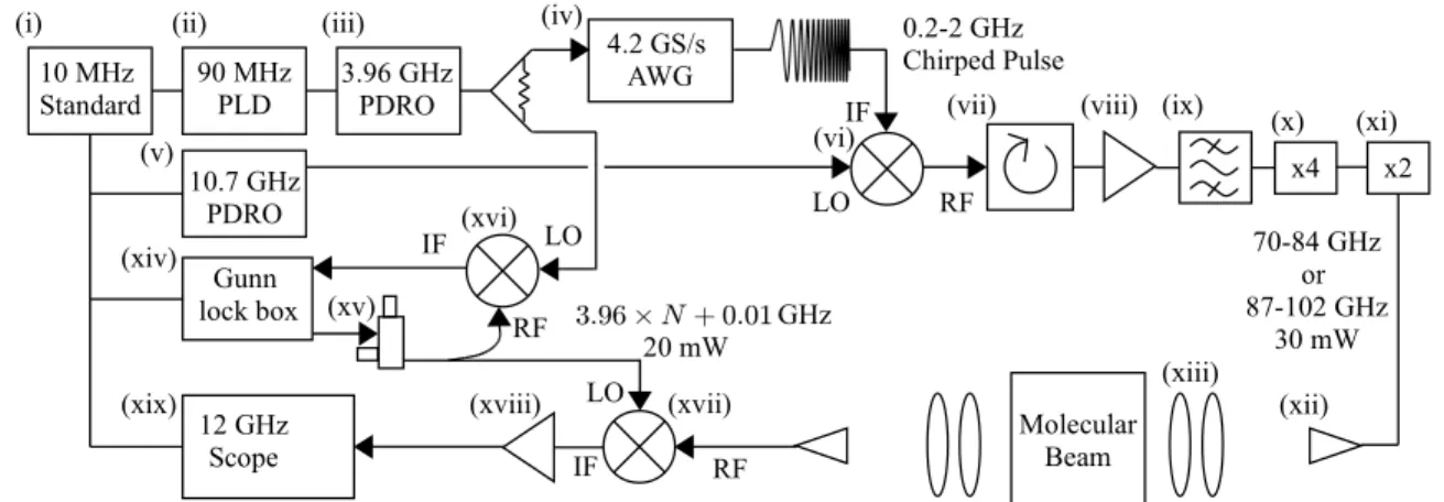
(28) 1.2. Spectrometer Design. The spectrometer is based on the CP-FTMW spectrometer of Pate and co-workers. 32 A schematic of the CPmmW spectrometer design is shown in Fig. 1-1. A 4.2 GS/s arbitrary waveform generator (AWG) is used to generate chirped pulses at frequencies in the range of 0.2–2 GHz. These pulses are up-converted by mixing with a phaselocked 10.7 GHz oscillator, and one of the sidebands is selected using a bandpass filter. Access to the millimeter-wave region is achieved by active multiplication (×8) of the resulting chirped microwave pulse. Because frequency multipliers multiply both the carrier frequency and the bandwidth of a chirped pulse, it is possible to generate chirped millimeter-wave pulses with ∼15 GHz bandwidth starting with a 0.2–2 GHz microwave pulse. As a result, the bandwidth of the AWG used in the experiment may be much narrower than that of the desired millimeter-wave chirped pulse. This was noted by Brown 𝑒𝑡 𝑎𝑙. in the bandwidth extension scheme designed for the FT-CPMW spectrometer. 32 Unlike the spectrometer of Pate and coworkers, which uses a traveling wave tube amplifier (TWTA) to achieve peak pulse powers of up to 300 W, the CPmmW spectrometer power is limited by the capabilities currently available of broadband Eand W-band amplifiers, which can attain peak powers of only ∼10–100 mW. Our system uses an active frequency doubler with an output power of 30 mW. Because the millimeter-wave power is low, horn antennas can be safely located outside of the molecular beam chamber. Teflon optics are used to focus the millimeter-wave radiation into the chamber through a set of teflon windows. The molecular FID must be down-converted to microwave frequencies for direct detection on a fast oscilloscope. This is achieved by mixing the collected signal with the output of a W-band Gunn oscillator. The detection bandwidth is limited by the 12 GHz oscilloscope [Tektronix model TDS6124C] used in the experiment. As in the design of Pate and coworkers, all oscillators and clocks used in the experiment are phase-locked to the same 10 MHz frequency standard. The experiment is repeated at an exact integer multiple of the period of the 10 MHz reference. This ensures that 28.

(29) (i). (ii) 90 MHz PLD. 10 MHz Standard. (iv). (iii). 0.2-2 GHz Chirped Pulse. 4.2 GS/s AWG. 3.96 GHz PDRO. (v). (xix). (xvi) IF. Gunn lock box. 12 GHz Scope. (vii). LO. RF. (viii) (ix). (x) x4. 10.7 GHz PDRO (xiv). IF (vi). (xv). LO. LO IF. (xvii) RF. x2. 70-84 GHz or 87-102 GHz 30 mW. RF 3.96 £ N + 0.01 GHz 20 mW (xviii). (xi). (xiii) Molecular Beam. (xii). Figure 1-1: Schematic diagram of the CPmmW instrument. For a full list of parts, see Section 1.10. All components of the experiment are phase locked to the same 10 MHz Rubidium Frequency Standard (i). A 4.2 GS/s AWG [Tektronix model AWG710B] (iv), operating at the 3.96 GHz rate of an external clock (iii), is used to generate a linearly-chirped pulse, which is up-converted (vi) by mixing with the output of a fixed-frequency 10.7 GHz oscillator (v). The resultant signal is isolated (vii) and amplified (viii). The desired sideband is then selected using a bandpass filter (ix) and actively frequency-multiplied by a factor of 8 (x and xi) to produce a chirped pulse that covers the 70–84 GHz or the 87–102 GHz frequency range with a peak power of 30 mW. The millimeter-wave pulse is coupled into free space using a 24 dBi standard gain horn (xii) and focused into a molecular beam chamber by a pair of teflon lenses (xiii). After the chirped excitation pulse has polarized the molecular sample, the FID is collected and down-converted (xvii) by mixing with the output of a Gunn oscillator (xv). The resultant signal is input to a low-noise amplifier (xviii) and averaged in the time domain on a 12 GHz oscilloscope (xix). the phase of the chirped pulse and the resultant FID is constant from pulse to pulse so that the signal can be phase-coherently averaged on an oscilloscope in the time domain.. 1.3 1.3.1. Power Limitation Measurement of Effective Power. The available power for the CPmmW spectrometer is currently limited to about 30 mW by the capabilities of commercially-available broadband millimeter-wave amplifiers. As millimeter-wave technology develops, more power is expected to become available in broadband solid-state devices. However, because of power limitations, 29.

(30) it is important to achieve efficient coupling of power into the molecular beam chamber so that the 𝐸-field of the radiation that interacts with the molecules is as high as possible. In order to evaluate the effective 𝐸-field in the interaction region, test measurements were performed on the 606 ← 515 𝑏-type pure rotational transition in SO2 at 72.758 GHz, for which the transition dipole moment (averaged over 𝑀𝐽 componenets) is 0.83 D. A resonant single-frequency pulse of varying duration was used to excite the transition.. The results, shown in Fig. 1-2, can be compared to an exponentially-damped Rabi oscillator. The detected signal, 𝑆, is the 𝐸-field radiated by the molecules, which is proportional to the magnitude of the quantum coherence, |𝑎0 𝑎1 |, evaluated at time 𝑡𝑝 , the pulse duration: (︂ 𝑆 ∝ |𝑎0 (𝑡𝑝 )𝑎1 (𝑡𝑝 )| = exp. )︂ −𝑡𝑝 | sin (𝜔𝑅 𝑡𝑝 )| 𝜏. (1.1). In Eq. 1.1, 𝜔𝑅 = 𝜇ℰ/~ is the on-resonance Rabi frequency, and 1/𝜏 is the decay rate of the coherence.. The data shown in Fig. 1-2 were fit to Eq. 1.1 to obtain best-fit parameters of 2.3 ± 0.2 𝜇s for 𝜏 and 1.11 ± 0.04 MHz for 𝜔𝑅 . The fit parameter for 𝜏 agrees with the measured 2.1 𝜇s 1/𝑒 dephasing time of the transition, which is dominated by the Doppler effect. The measured Rabi frequency corresponds to an effective 𝐸-field of 42 V/m. The measured diameter of the millimeter-wave focus (containing 90% of the integrated 𝐸-field) from the teflon lenses is ∼2.5 cm. If 30 mW of power were ideally focused onto a (2.5 cm)2 area, it would result in a 195 V/m 𝐸-field. Part of the loss of effective 𝐸-field is due to power loss. There are unavoidable losses due to reflections in the horn antenna and from the surfaces of the lenses and chamber windows. However, horn-to-horn transmission loss is only ∼3 dB (corresponding to a loss of 30% in 𝐸-field). The remaining loss of effective 𝐸-field can be attributed to imperfections in the profile and focussing of the millimeter-wave beam. 30.

(31) '%*. ! "# "!. &%$#"!. $# $! # ! !. $. ". %. '()* !". '3*. "# "!. &%$#"!. $# $! # ! !. $!. "!. !. %!. #+,"-&./'012*. Figure 1-2: a) The amplitude of the FID signal from the SO2 606 ← 515 transition is plotted as a function of the duration of the single frequency excitation pulse. The data were fit to Eq. 1.1 to obtain best-fit parameters 𝜏 = 2.3 ± 0.2 𝜇s and 𝜔𝑅 = 1.11 ± 0.04 MHz. b) The signal amplitude from the same transition is plotted as a function of millimeter-wave pulse power attenuation, for a constant pulse duration of 𝑡𝑝 = 2 𝜇s. The solid curve is the signal amplitude predicted by Eq. 1.1 with the best-fit parameters from above. The 𝐸-field plotted on the 𝑥-axis was calculated from the best-fit value of 𝜔𝑅 at zero attenuation and scaled according to the variable attenuation. 31.

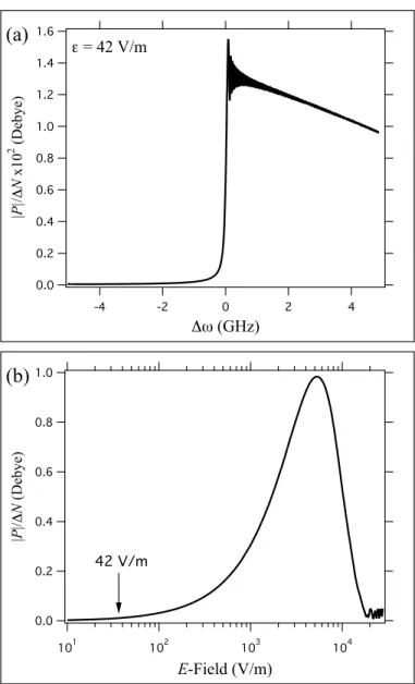
(32) 1.3.2. Power Requirements for Broadband Chirped Pulses. To calculate the achievable polarization of a two-level system excited by a broadband chirped millimeter-wave pulse, we integrate the optical Bloch equations for the case of a linearly-chirped pulse, as given by McGurk 𝑒𝑡 𝑎𝑙. 36 We define the polarization in the form 𝑃 = (𝑃𝑟 + 𝑖𝑃𝑖 )𝑒𝑖(𝜔𝑡−𝑘𝑧) + c.c.. (1.2). The time-dependent 𝐸-field of the excitation pulse is 1 𝐸 = 2ℰ cos (𝜔𝑖 𝑡 + 𝛼𝑡2 ) 2. (1.3). = 2ℰ cos {[𝜔0 − Δ𝜔(𝑡)] 𝑡}, where we define 𝛼 as the linear frequency sweep rate and Δ𝜔 as the detuning of the excitation pulse from the two-level system resonance, 𝜔0 . The Bloch equations can be written for the polarization in terms of Δ𝜔 36 𝑑𝑃𝑟 𝑃𝑟 + Δ𝜔𝑃𝑖 + =0 𝑑(Δ𝜔) 𝑇2 𝜇2 ℰ 𝑃𝑖 𝑑𝑃𝑖 − Δ𝜔𝑃𝑟 + Δ𝑁 + =0 𝛼 𝑑(Δ𝜔) 2~ 𝑇2 ~ (Δ𝑁 − Δ𝑁0 ) 𝛼~ 𝑑(Δ𝑁 ) ℰ = 0. − 𝑃𝑖 + 4 𝑑(Δ𝜔) 2 4 𝑇1 𝛼. (1.4). In Eq. 1.4, 𝑇1 and 𝑇2 are the familiar decay lifetimes of the population and coherence, respectively, and Δ𝑁 is the population difference. Equation 1.4 was numerically integrated and the results are shown in Fig. 1-3. Figure 1-3 demonstrates that the polarization achievable in a typical small molecule across a bandwidth of 10 GHz with a 42 V/m electric field is only 1% of the maximum polarization that would be achievable if higher chirped-pulse power were available. A qualitative difference between the polarization achieved with a broadband chirped pulse and that achieved with a single-frequency excitation pulse (Figure 1-2) is that even in the absence of relaxation effects, recurrence of the polarization does not take place at high 𝐸-field in the chirped-pulse case. This is a well known 32.

(33) !". '7,. !#. ". "8"9&"5!6. &. !% %!&. !. " !. ,)+*)('" %$#". !$. %!" %!# %!$ %!% '#. '$. !. %. $. #. "'-./,. !%. '*,. %!&. ". ,)+*)('". %!". !. %!#. #$)*+,. %!$ %!% %. %$. %(. #. %#. 012)34"'5!6,. Figure 1-3: Equation 1.4 was numerically integrated for the case of a 10 GHz bandwidth chirped pulse of 1 𝜇s duration exciting a 1 D dipole moment with 𝑇1 and 𝑇2 of 10 𝜇s and 2 𝜇s, respectively. The two level system resonance is assumed to occur at the center of the excitation pulse bandwidth. (a) The integration of Eq. 1.4 is shown for the above parameters with an 𝐸-field of 42 V/m, which is the available 𝐸-field in the current spectrometer. The magnitude of the polarization is plotted. (b) The 𝐸-field (ℰ) was varied and the resultant polarization after the excitation pulse is plotted. Optimal polarization occurs at an 𝐸-field of ∼4000 V/m. The polarization never quite reaches its maximum value of 1 D because a small amount of dephasing occurs during the excitation pulse. Note that the polarization achieved at 42 V/m corresponds to only ∼1.5% of the maximum achievable polarization.. 33.

(34) √ phenomenon in the adiabatic fast passage regime. When 𝜇ℰ/~ 𝛼 ≫ 1, the effective 𝐸-field vector in the Bloch polarization picture is very strong and moves slowly relative to the Rabi precession. The polarization vector precesses tightly around the 𝐸-field vector as it is swept through 180∘ , and the system is swept slowly through resonance until population inversion is achieved. 37 √ In the weak field case (𝜇ℰ/~ 𝛼 ≪ 1), the signal scaling has been solved by McGurk 𝑒𝑡 𝑎𝑙. 36 They found that 𝑃 ∝. 𝜇2 ℰΔ𝑁 √ . 𝛼. (1.5). The polarization will also decay at a rate proportional to 𝑇1−1 + 𝑇2−1 . Therefore, the excitation must occur on a timescale short compared to these time constants. Given that the excitation pulse duration is constrained, the obtainable signal is proportional to the reciprocal square root of the bandwidth. As pointed out by Brown 𝑒𝑡 𝑎𝑙., 32 this means that the chirped-pulse signal scales favorably as bandwidth is increased. In contrast, the signal obtained from a Fourier-transform limited pulse scales as the reciprocal of the bandwidth to the first power. It is possible to achieve more polarization from a given transition by decreasing the bandwidth of the chirped pulse. However, this is rarely an advantageous strategy for increasing the efficiency of spectral acquisition, because the increase in signal is only proportional to Δ𝜔 1/2 . Breaking up a spectrum into more than one frequency region therefore does not decrease the averaging time needed to obtain a specified signal-to-noise level over a given frequency region, since the noise reduction also scales as the square root of the number of averages, and there is a cancelation between the signal increase and the required number of averages. √ In the strong power regime (where 𝜇ℰ/~ 𝛼 is no longer ≪ 1), the maximum achievable polarization is limited by 𝑃𝑚𝑎𝑥 = 𝜇Δ𝑁 . The maximum obtainable polarization from a given sample does not scale with the chirp bandwidth or the 𝐸-field, and only scales as 𝜇 to the first power. 34.

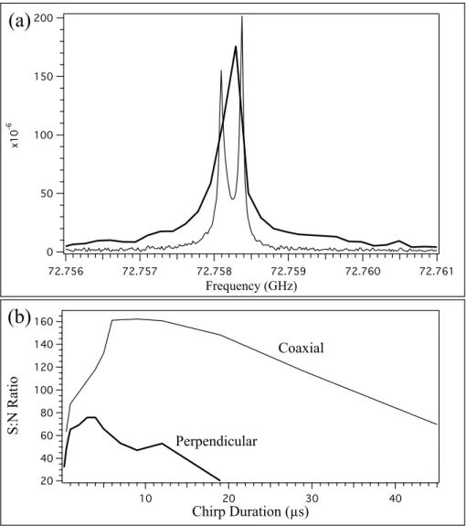
(35) 1.4. Shorter Dephasing times. In addition to low power availability, another challenge that faces chirped-pulse spectroscopy in the millimeter-wave region is that the dephasing time of the molecular transitions tends to be much shorter than in the centimeter-wave region. In a supersonic expansion, the most significant contributor to the lifetime of the FID is usually the Doppler-limited 𝑇2 broadening. Since the Doppler effect is proportional to the emitted frequency, the dephasing times for the millimeter-wave FIDs are an order of magnitude shorter than those measured with centimeter waves. Pate and coworkers report FID lifetimes of ∼10 𝜇s below 20 GHz, 32,33 while we encounter lifetimes of ∼2 𝜇s. As a result of the shorter dephasing time, the millimeter-wave chirped pulse must have a shorter duration in order to minimize the dephasing that occurs during the polarizing pulse. This faster dephasing is combined with the additional problem of low available millimeter-wave power, and as a result the CPmmW spectrometer must operate in the low power limit when used to study rotational spectra of molecules with ∼1 D dipole moments. One way to overcome Doppler dephasing in millimeter wave molecular beam experiments is to change the experimental geometry to reduce the Doppler profile. This has been employed with our CPmmW spectrometer by using a rooftop reflector and a wire-grid polarizer to propagate the millimeter-wave radiation parallel and antiparallel with the molecular beam in a manner similar to that used previously to obtain high-resolution spectra with our sequential scanning millimeter-wave absorption spectrometer. 38 The co-propagating geometry removes most of the Doppler effect caused by the component of the molecular velocity perpendicular to the molecular beam direction. In Fig. 1-4, a comparison is made between the signal obtainable with and without the rooftop reflector geometry. The linewidth was reduced from 350 kHz to 66 kHz. Because the FID lifetime is lengthened by a factor of 5, it is possible to extend the chirp duration without loss due to dephasing. This leads to stronger polarization of the sample and more signal. Additional advantage in the signal-tobackground-noise ratio arises from the fact that the line is narrower. 35.

(36) ).-. !!. "#!. '&%!"$. "!!. #!. ! ( )(#&. ( )(#(. ( )(#+. ( )(#*. !"#$"%&'()*+,-. ( )(&!. ( )(&". )<- "&! ",!. 65.=4.>. " !. 543.2(10/. "!! +! &!. ?"!8"%@4&$>.!. ,! ! "!. !. -!. 674!8(9$!.345%():;-. ,!. Figure 1-4: A comparison is made between the signal obtained from the 606 ← 515 transition of SO2 in the perpendicular millimeter wave/molecular beam geometry (thick curve) and coaxial geometry obtained using a rooftop reflector (thin curve). The Doppler-limited linewidth is narrower in the coaxial geometry. The line is split into its two Doppler components when this double-pass configuration is used (a). Because the FID lifetime is longer when the Doppler dephasing is minimized, the duration of the excitation chirp can be extended to achieve further improvement in signal strength. In panel (b), the signal-to-background-noise ratio is plotted as a function of the chirp duration for both geometries. The millimeter-wave power, gas expansion characteristics, and other parameters were held constant.. 36.

(37) The colinear geometry can also be used to improve the resolution, as demonstrated in the case of the 𝐽 = 5 ← 4, 𝐾 = 0 transition of acetonitrile with resolved hyperfine structure due to the. 1.5. 14. N quadrupole moment (Fig. 1-5).. Phase Stability. Another difficulty with up-converting the chirped-pulse technique into the millimeterwave region is that the experiment becomes more sensitive to phase instabilities. When the signal is frequency-multiplied by 8, any phase jitter is also multiplied by 8. Phase jitter might be attributed to to temperature fluctuations and mechanical vibrations in the laboratory, or to phase jitter characteristics of electrical components. When using chirped-pulse techniques, two types of phase jitter are possible: 𝑡jitter as illustrated in Eq. 1.6a or 𝜑-jitter, as illustrated in Eq. 1.6b.. [︂. ]︂ 1 2 𝐼 ∝ sin 𝜔0 (𝑡 + Δ𝑡) + 𝛼(𝑡 + Δ𝑡) + 𝜑 2 [︂ ]︂ 1 2 𝐼 ∝ sin 𝜔0 𝑡 + 𝛼𝑡 + (𝜑 + Δ𝜑(𝜔)) 2. (1.6a) (1.6b). We find that when the phase of the FID is unstable from one acquisition to the next, the instability can be corrected by rotating the phases of the Fourier transforms relative to one another (and not by shifting the FIDs in time). Furthermore, we find that the rotation angle that maximizes the overlap between the two Fourier transforms is independent of the frequency. That is, in Eq. 1.6b, Δ𝜑(𝜔) = Δ𝜑. Thus, Eq. 1.7 can be used to rotate the phase of the Fourier transform to correct for phase instabilities: ⎛ ⎞ ⎛ ⎞⎛ ⎞ ′ ℜ{𝐹 (𝜔)} cos Δ𝜑 sin Δ𝜑 ℜ{𝐹 (𝜔)} ⎝ ⎠=⎝ ⎠⎝ ⎠, ′ ℑ{𝐹 (𝜔)} − sin Δ𝜑 cos Δ𝜑 ℑ{𝐹 (𝜔)}. (1.7). where ℜ{𝐹 (𝜔)} and ℑ{𝐹 (𝜔)} refer to the real and imaginary parts of the Fourier transform, respectively. The frequency-independence of the correction indicates that the source of the 37.

(38) 2?6. '"'! '"''. 8'"'! '. 9. !'. !9. :;<+12=>6. &'. 276. !" #((. !" #(#. !" #$'. )*+,-+./0123456. !" #$&. !" #$%. Figure 1-5: High-resolution CPmmW spectrum of the acetonitrile 𝐽 = 5 ← 4, 𝐾 = 0 transition with resolved 14 N quadrupole moment hyperfine structure. The FID (a) has a decay constant of ∼17 𝜇s. The Hamming window function was used in the Fourier Transform. The spectrum (b) is Doppler-doubled as a result of the rooftop reflector geometry. The line spectrum represents the calculated spectrum obtained using the accepted nuclear quadrupole coupling constant, −4.2244 MHz, 39 and a best-fit molecular beam velocity of 508 m/s. The thick central line is the measured central line frequency and the dotted line is the unresolved line position reported by Boucher 𝑒𝑡 𝑎𝑙. 40 The measured line frequency agrees to within the 60 kHz reported uncertainty.. 38.

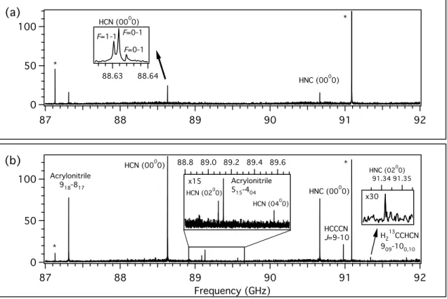
(39) phase instability is likely to be in one of the single-frequency local oscillators. If the phase jitter were generated in a component that passes a chirped pulse, there would likely be frequency dependence to the phase jitter, since different frequencies accumulate phase at different rates. In future generations of our spectrometer, we plan to replace the Gunn oscillator with a multiplied phase-locked microwave oscillator as the local oscillator for the down-conversion. This will allow us to determine whether the Gunn oscillator is the source of phase instability. Long-term drifts in phase of the type discussed above have been efficiently corrected in signal processing. This type of instability can be corrected by rotating the phase of the Fourier transform of each acquisition (Eq. 1.7) by the angle Δ𝜑 that maximizes the overlap of the strongest line in the spectrum. Because of the frequency independence of Δ𝜑, this rotation maximizes the phase overlap of all molecular lines, regardless of how far apart they are in frequency. When it is necessary to perform a long average over the course of an hour or more, the averaging can be performed in shorter 5–10 minute acquisitions over which time the phase of the FID is stable. These shorter acquisitions can then be phase corrected with signal processing tools before being averaged together. The overall time required for the acquisition of the long average is affected negligibly because the data must be Fourier-transformed and stored only once every 5–10 minutes when this scheme is implemented. A disadvantage of this method is that it is only efficient when there is a strong line that is visible above the baseline noise after a 5–10 minute acquisition. If necessary, the phase correction can be achieved by introducing into the sample mixture a standard that has a strong transition. The phase-correction algorithm can be applied automatically in the LabView program that is used to collect and average the data. As an example, we have acquired 87–92 GHz spectra of the 193 nm photolysis products of acrylonitrile. We collected 28,000 averages in acquisitions of 500–2000 averages each. In Fig. 1-6 we present a comparison between the spectra obtained when each acquisition is phase corrected and when each acquisition is not phase corrected. Note that the levels of background noise in the two spectra are similar, but the signal in the phase-corrected spectrum is several times stronger, because signal is destroyed 39.

(40) when individual FIDs are averaged out of phase. In the phase-corrected spectrum, the signal-to-background ratio increases as the square root of the number of acquisitions out to the longest measurement of 28,000 acquisitions.. 1.6 1.6.1. Evaluation Spectroscopy of Ground States. We used the frequency region surrounding the 72,976.7794 MHz OCS 𝐽 = 6 ← 5 transition to compare the CPmmW spectrometer to the supersonic jet W-band bolometer-detected absorption spectrometer used previously in the Field laboratory (Fig. 1-7). 38,41 The older absorption spectrometer was used primarily for measuring hyperfine structure surrounding lines with known positions and was not designed for broadband spectral acquisition. With the absorption spectrometer, only a narrow 100 MHz region containing the main OCS 𝐽 = 6 ← 5 transition could be scanned during the 100 minute experiment (Fig. 1-7.a). However, with the CPmmW spectrometer, a 4 GHz spectral region could be surveyed at improved signal-to-background-noise ratio in approximately half the time. The strong OCS 𝐽 = 6 ← 5 transition is visible above the background noise after only seconds of averaging. After 5 minutes of averaging, the spectrum reaches a signal-to-background-noise ratio comparable to that obtained with the absorption spectrometer. The spectrum shown in Fig. 1-7.b was obtained in 50 minutes and exhibits greater than two-fold improvement in signal-to-background-noise ratio over the spectrum shown in Fig. 1-7.a. Because the broadband Fourier-transform capabilities of the CPmmW spectrometer can be used to survey a broad spectral region, it is possible not only to find the strong OCS 𝐽 = 6 ← 5 transition after mere seconds of averaging, but also to observe simultaneously the weaker satellite transitions, which are assigned to isotopologues and vibrationally excited states of OCS. From the signal to background noise ratio of the O13 CS peak, we estimate that for the bandwidth and acquisition time used in this experiment, the limit of detection for OCS 𝐽 = 6 ← 5 transition is approximately 40.

(41) 0B4. 5. 2=</0!!!!4 !>!; !> ;. !!. !>!;. "! !. 0A4 !!. 5. %&. %%CD?. %%CDE. %%. 6-(.78,9:(97) ////# %;% &. 2=</0!!!!4. 2<=/0!!!!4. %#. #!. %%C% %#C! %#C$ %#CE %#CD F ". 2=</0!$!!4. 6-(.78,9:(97) " ";E!E. 2<=/0!!!!4. 2===</ >#; !. 5. %&. !. 5. 2=</0!E !4. "! !. #. %%. %# #! '()*+),-./01234. #. #$. 2<=/0!$!!4 # C?E # C?". F?!. 2$ ?==2=< #!#; !!@ !. #$. Figure 1-6: A 5-GHz bandwidth spectrum of the 193 nm photolysis products of acrylonitrile was acquired in a supersonic jet expansion. A total of 28,000 averages were recorded in short acquisitions of 500–2000 averages each. Without phase correction (a), only the acrylonitrile 𝐽𝐾𝑎 𝐾𝑐 = 918 ← 917 , the HCN (𝜈1 𝜈2ℓ 𝜈3 ) = (0 00 0), 𝐽 = 1 ← 0 line, and the HNC (0 00 0), 𝐽 = 1 ← 0 lines are detected above the noise. When the phase of each spectrum is shifted to maximize the overlap of the HCN (0 00 0) line (b), the signal-to-background-noise ratio increases dramatically and more lines become visible: HCN (0 20 0), 𝐽 = 1 ← 0; HCN (0 40 0), 𝐽 = 1 ← 0; HNC (0 20 0), 𝐽 = 1 ← 0; acrylonitrile 515 ← 404 ; HCCCN, 𝐽 = 10 ← 9 and a 13 C-substituted acrylonitrile line at 91,821.43 MHz. Artifact lines corresponding to local oscillator frequencies are labeled with asterisks.. 41.

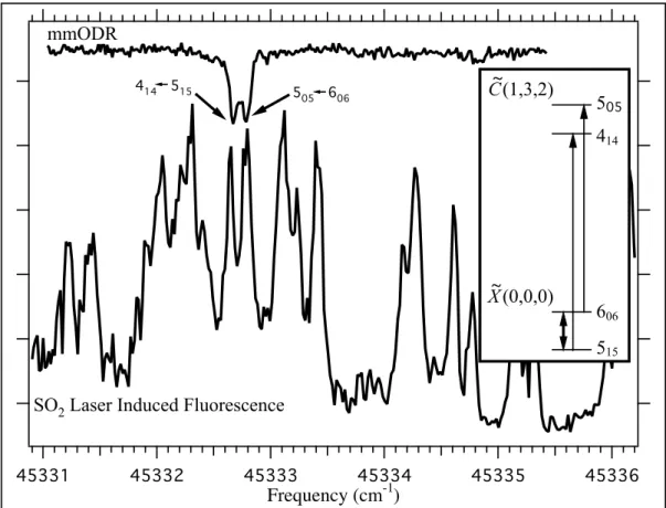
(42) 1011 molecules/cm3 . The CPmmW spectrometer has also been used in millimeter wave-optical double resonance (mmODR) experiments. In the first such implementation, the millimeterwave beam was crossed with the frequency-doubled output of a pulsed dye laser. The supersonic jet expansion was directed at a right angle to the millimeter-wave and laser beams. The 606 ← 515 transition in ground-state SO2 was excited by the millimeter ˜ 1 B2 (1, 3, 2) ← X ˜ 1 A1 (0, 0, 0) waves and the laser frequency was scanned across the C band centered at 45336 cm−1 . The ∼10 ns laser pulse arrived 500 ns after the start of the millimeter-wave FID, so that it causes a decrease in the magnitude of the millimeter-wave coherence if it is resonant with one of the two states involved. The method is similar to the cavity Fourier-transform microwave-optical double resonance technique of Nakajima 𝑒𝑡 𝑎𝑙. 42 The double resonance spectrum was obtained by recording the normalized ratio of the FID intensity before and after the laser pulse. The double resonance spectrum is plotted along with the laser induced fluorescence (LIF) spectrum in Fig 1-8. Rotational assignments for this band have been made previously by Yamanouchi 𝑒𝑡 𝑎𝑙. 43 The double resonance peak at 45332.65(2) cm−1 agrees to within experimental uncertainty with the peak assigned to the 414 ← 515 transition. We have assigned the other peak at 45332.79(2) cm−1 to the 505 ← 606 transition, which was not assigned by Yamanouchi 𝑒𝑡 𝑎𝑙. due to spectral congestion and complications caused by Coriolis effects. Both of our assignments are confirmed by the existence of combination difference peaks in the LIF spectrum. The successful implementation of mmODR with our spectrometer suggests that the technique could be used to generate two dimensional Chirped-Pulse mmODR spectra in order to decongest LIF spectra and provide rotational assignments. The technique will provide the most information for molecules with sufficiently small rotational constants such that the chirped pulse will cover several rotational transitions. The laser spectrum can be scanned while many ground-state rotational transitions are probed, and the Fourier transform of the FID dip will provide information about which ground-state rotational level is involved in each LIF transition. 42.

(43) (a). OCS (J = 6-5). Bandwidth = 100 MHz S:N = 670 Acquisition Time = 100 min. (b) OC34S. 72.975 72.976 72.977 72.978. O13CS. OCS (v2 = 1). x 35 Bandwidth = 4 GHz S:N = 1500 Acq. Time = 50 min. 72.740. 71.0. 71.5. 72.0. O13CS. 72.742. 72.5. 72.744. 72.975 72.976 72.977 72.978. 73.5 73.0 Frequency (GHz). 74.0. 74.5. Figure 1-7: For comparison, the spectrum of OCS in the region surrounding the 𝐽 = 6 ← 5 region was measured with (a) the scanned absorption spectrometer previously used in the Field group and (b) the CPmmW spectrometer. The CPmmW spectrometer was able to cover 40 times the bandwidth in half the time with better signal-to-background-noise ratio. Differences in line profile are due primarily to the fact that the CPmmW spectrometer detects electric field, which is proportional to the square root of power.. 43.

(44) !"# %. &&&!%!. !'!&&&#'#. (. !&97:<:%;. (. &98:8:8;. 4'! 575. 686 474. $!%&'()*+&,-./0*.&12/3+*)0*-0* !""%. !""$. !""" !"" !"#$"%&'()&*+,-. !""!. !""#. ˜ Figure 1-8: The LIF spectrum of SO2 (lower trace) to the (1, 3, 2) level of the C state is shown along with a millimeter wave-optical double resonance spectrum to the same band (upper trace). The scheme for the double resonance experiment is shown in the inset. The thick double arrow represents the millimeter-wave coherence that ˜ 0, 0) state. The was generated between the 606 and 515 rotational levels of the X(0, double resonance signal was obtained by measuring the dip in the millimeter-wave FID intensity as the laser was scanned.. 1.6.2. Spectroscopy of Laser-Excited States. CPmmW spectroscopy is particularly advantageous as a tool for probing laser-excited states since it is designed for pulsed operation and can be easily coupled to pulsed supersonic jets and tunable pulsed laser systems. The duty cycle of such experiments is necessarily low. In our laboratory, the pulsed dye lasers operate at 10 Hz and the chirped-pulse experiment lasts ∼5 𝜇s or less. Thus the fraction of time when microwave observations can be made is less than 10−4 , when compared with traditional non-pulsed absorption measurements. CPmmW spectroscopy is well suited to this case since it can record a broad spectral region during the short radiative lifetime and 44.

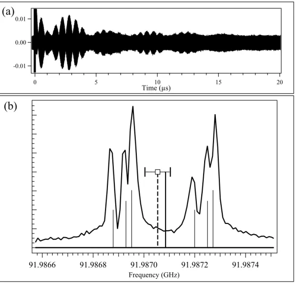
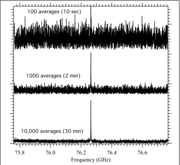
(45) the time between gas pulses can be used for digital averaging of the FID. As a demonstration that CPmmW spectroscopy can be used to probe laser-excited states, we measured the (𝐽 ′ = 2, 𝑁 ′ = 2) ← (𝐽 ′ = 1, 𝑁 ′ = 1) transition in the excited triplet electronic state e 3 Σ− (𝜈 = 2) of CS using a 1 GHz bandwidth chirped pulse (Fig. 1-9). Because the uncertainty in laser transitions is typically ∼1 GHz, it may be necessary to cover a broad spectral range when probing for rotational transitions of laser-excited states. The CS line could be seen above the noise after about 100 averages (10 seconds). We estimate that this signal came from a total of ∼ 4.8 × 1010 excited CS molecules in a single quantum state.. 100 averages (10 sec). 1000 averages (2 min). 10,000 averages (30 min). 75.8. 76.0. 76.2 76.4 Frequency (GHz). 76.6. Figure 1-9: The e 3 Σ− (𝜈 = 2) state of CS was populated using the frequency-doubled output of a tunable Nd:YAG-pumped dye laser at ∼39910 cm−1 . The (𝐽 ′ = 2, 𝑁 ′ = 2) ← (𝐽 ′ = 1, 𝑁 ′ = 1) transition in the excited state was then probed using a 1 GHz bandwidth chirped pulse centered on the transition. 45.

(46) The transition frequency was previously reported as 76,229.027(20) MHz. 44 In the current work, we correct this frequency to 76,263.89(10). The FWHM is 1.1 MHz and is attributable to the radiative lifetime of the e 3 Σ− state. The difference between the previously reported frequency and the current value is almost exactly 35 MHz, which was the reference frequency used in the original measurement to stabilize the Gunn oscillator. This suggests that the oscillator may have been erroneously locked to the second harmonic of the reference. The CPmmW technique has also been recently applied to pure electronic RydbergRydberg transitions in calcium atoms. 9. 1.7. Instrument Noise Floor. In our current spectrometer, the noise level is set by the noise output of the source amplifier. We experimentally measure the noise level at the receiver to be a factor of 9 in power above the thermal noise at the receiver. Fast, broadband PIN switches with insertion losses of ∼2 dB have recently become available for the W-band. We plan to place a switch after the source amplifier to eliminate source amplifier noise during detection of the FID. The noise encountered in the experiment will then be set by the noise figure of the detection arm. In the current spectrometer, the noise figure of the detection arm is set by a combination of a rather lossy downconverter (9 dB conversion loss) and the 2.3 dB noise figure of the low noise amplifier for the RF. The combined noise figure after the collection horn is therefore ∼11.3 dB (or a factor of 13.5). Recently, LNAs covering the full W-band with a noise figure of ∼5 dB have become available. Such an amplifier would need to be protected from the powerful excitation pulse by a switch (∼2 dB insertion loss). The combined noise figure of the detection arm would then be set by these two components to 7 dB (or a factor of 5.0). We therefore expect to be able to achieve an overall reduction in noise floor by a factor of 13.5 × 9/5.0 = 24 in power or 4.9 in electric field. The 2 dB insertion loss of the switch on the source will cause a 25% loss in signal, but this will be more than compensated by the reduction in noise floor. 46.

(47) 1.8. Future Work. CPmmW spectroscopy is shown to be an advantageous method for spectroscopy in the 70–100 GHz region. However, future work is planned to improve the sensitivity of the method by taking full advantage of recent advances in millimeter-wave technology. Most importantly, we plan to obtain W-band low-noise amplifiers and switches to improve the noise floor of the detection arm, as discussed in Section 1.7. We also hope to obtain new power amplifiers to increase the strength of our excitation pulse. Technology is rapidly progressing for broadband millimeter-wave power amplifiers. Powers up to 400 mW have been reported across the W-band. 45,46 Because signal scales with the square root of pulse power, such an amplifier (used in conjunction with a 2 dB insertion loss switch) would improve the signal strength in the CPmmW spectrometer by a factor of 3.. 1.9. Acknowledgments. The authors are grateful for advice and support from Brooks Pate and his lab. This work was supported at MIT by DOE Grant No. DEFG0287ER13671 and by an NSF Graduate Research Fellowship.. 1.10. Appendix: Part List. The following part list is labeled with Roman numerals corresponding to the labeling in Fig. 1-1. In cases where parts are swapped out depending on which sideband is being used, the parts are labeled “a” for the lower (70–85 GHz) sideband and “b” for the upper (87–102 GHz) sideband. i. 10 MHz Rubidium Frequency Standard (Stanford Research Systems FS725) ii. 90 MHz Phase-Locked Crystal Oscillator (Miteq PLD-10-90-15P) iii. 3.96 GHz Phase-Locked Dielectic Resonator Oscillator (Microwave Dynamics PLO-2000-03.96) 47.

(48) iv. 4.2 GS/s Arbitrary Waveform Generator (Tektronix AWG710B) v. 10.7 GHz Phase-Locked Dielectric Resonator Oscillator (Miteq PLDRO-10-107003-8P) vi. Double-Balanced Mixer (Macom M79) vii. 8–16 GHz circulator (Hitachi R3113110) viii. 1.5–18 GHz amplifier (Armatek MH978141) ix.a. 8.7–10.5 GHz bandpass filter (Spectrum Microwave C9680-1951-1355) ix.b. 10.9–12.7 GHz bandpass filter (Spectrum Microwave C11800-1951-1355) x. Q-Band Active Frequency Quadrupler (Phase One Microwave PS07-0153A R2) xi.a. E-Band Active Frequency Doubler (Quinstar QMM-77151520) xi.b. W-Band Active Frequency Doubler (Quinstar QMM-9314152ZI1) xii. WR10 gain horn, 24 dBi gain mid-band (TRG 861W/387) xiii Teflon circular lenses, 30 cm and 40 cm focal length at 80 GHz (custom) xiv. Gunn Phase Lock Module (XL Microwave Model 800A) xv. W-Band Gunn Oscillator (J.E. Carlstrom Co.) xvi. W-Band Subharmonic Downconverter (Pacific Millimeter Products) xvii.a. E-Band Downconverter (Ducommun Technologies FDB-12-01) xvii.b. W-Band Downconverter (Ducommun Technologies FDB-10-01) xviii. Low-Noise Amplifier (Miteq AMF-5D-00101200-23-10P) xix. 12 GHz Digital Storage Oscilloscope (Tektronix TDS6124C). 48.

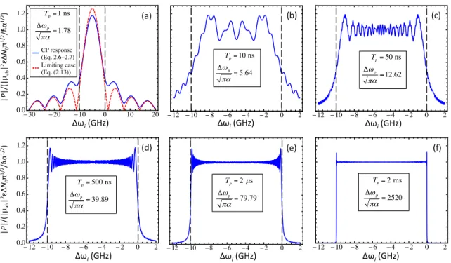
(49) Chapter 2 Edge effects in chirped-pulse Fourier transform microwave spectra Abstract Recent applications of chirped-pulse Fourier transform microwave and millimeter wave spectroscopy have motivated the use of short (10–50 ns) chirped excitation pulses. In this regime, individual transitions within the chirped pulse bandwidth do not all, in effect, experience the same frequency sweep through resonance from far above to far below (or vice versa), and “edge effects” may dominate the relative intensities. We analyze this effect and derive simplifying expressions for the linear fast passage polarization response in the limit of long and short excitation pulses. In the long pulse limit, the polarization response converges to a rectangular function of frequency, and in the short pulse limit, the polarization response morphs into a form proportional to the window function of the Fourier-transform-limited excitation pulse.a. 2.1. Introduction. Chirped-pulse Fourier-transform microwave (CP-FTMW) spectroscopy, invented in Professor Brooks Pate’s lab, 32,34 is rapidly becoming a mainstream technique for broadband (> 10 GHz) high-resolution microwave and millimeter-wave spectroscopy. Because the CP-FTMW technique allows rapid acquisition of broadband rotational spectra, it provides a wealth of chemical and physical information that was not previa. At the time of the submission of this thesis, the contents of this chapter have been submitted for publication in The Journal of Molecular Spectroscopy.. 49.