MIT Sloan School of Management
MIT Sloan School Working Paper 5519-18
The Dynamics of Competition
and of the Diffusion of Innovations
James M. Utterback, Calie Pistorius, and Erdem Yilmaz
This work is licensed under a Creative Commons Attribution-NonCommercial License (US/v4.0)
http://creativecommons.org/licenses/by-nc/4.0/ August 21, 2018
The Dynamics of Competition and of the Diffusion of Innovations
1 Introduction
Our purpose in this paper is to briefly review the evolution of our understanding of the emergence and diffusion of innovation, and to provide a new and more nuanced model of diffusion. Our point of departure will be to abandon the idea that innovation results only in pure competition, or a zero-‐sum game, between the new and the established practices. Given evidence from many cases, we believe it more likely that at least at the beginning of races between new and older products, processes and services, growth of one will often stimulate growth of the others. We will term this symbiotic competition. Later the interacting technologies may fall into equilibrium, or a perhaps cyclic state that we will term
predator-‐prey competition, and finally a zero-‐sum game of pure competition in economic
terms may ensue. This has significant implications with regard to innovation strategy.
We do not intend our work to be a forecast of technological trajectories or futures. Rather looking at generations of products, processes and services and how they evolve should help us to think systematically rather than incrementally. Thinking systematically should help us avoid the risk of lengthy and lavish overinvestment in dying businesses, which is often the case observed. Thinking systematically should also help us grasp opportunities that provide premium growth.
We will show how our model of the dynamics of competition and diffusion of innovations can be simply and practically applied and will provide a few examples analyzing the emergence of new products and services. An open source software package for determining coefficients of competition and rates of diffusion is available for interested users. The model and software do not require traditional simplifying assumptions and subsume earlier formulations and models.
2 Motivation, contributions and plan
Why is diffusion of innovation important? Ideas and inventions are major sources of both economic growth and of the expansion of human possibilities. In order for ideas to matter though, they must not only be reduced to practice, but their application must also spread or diffuse among potential users. Ideas and inventions are sometimes seen as sweeping established practices aside and somewhat hysterically as displacing or disrupting whole swathes of industry. Who though would agree that we should give up electric light and return to gas lighting or that using ice for refrigeration is more natural, convenient and efficient that an electric refrigerator and freezer? Would anyone wish to give up a mobile phone to return to land lines and pay phones?
The point is not that major adjustments were not required or that whole new industrial ecologies did not need to arise to put these new ideas into practice. Rather it is that each displacement led to broader use and possibilities for illumination, refrigeration and communication, greater efficiencies, increases in quality and much expanded markets. Moreover, the spread of electric generation and distribution networks led to many other industrial applications and household conveniences. The rise of refrigeration led to air conditioning and great expansions of cities and land values in previously oppressive climates. Mobile devices have led to the convergence of cameras, music players, maps and
location finding and a myriad of other functions and uses into a single iconic object, instead of just creating a device, which allows us to ‘talk anywhere.’
How does the diffusion of new products, processes and services occur? Everett Rogers (1962) conceived of innovation as something entirely new expanding into an unoccupied market. Rogers famously described different phases in the diffusion process in which customers with different inclinations played distinct roles in sequence with earlier adopters persuading and influencing those more slowly convinced and more reluctant to adopt. Rogers’ equations make the growth rate of an innovation in the market proportional to the filled niche compared to the unfilled market niche resulting in a logistic curve. Modeling diffusion thus requires an estimate of potential market size.
John Norton and Frank Bass (1987) were among the first to consider a new product or process generation replacing a prior one. Their model importantly allows for both the growth and later decline in the use of a product and assumes a growing market from generation to generation. The model has been applied simultaneously to multiple generations, such as semiconductor memory chips of increasing capacity. Norton and Bass implicitly assume that different generations of a product or device are in pure competition with one another. Thus, sales of generation one may be declining toward zero while generation two has reached its height and a new generation three is beginning to grow. Norton and Bass’ model applies to many products, but as we will show later, clearly not all. Various purely empirical efforts to estimate diffusion rates followed the early pioneers including that of John Fisher and Robert Pry of General Electric. Fisher and Pry (1971) modeled the diffusion of a new product or process becoming a substitute for a prior one as being proportional to F/(1-‐F) plotted on a log scale, where F is the market share of the emerging product or process in question versus time. They examined dozens of cases from margarine replacing butter to basic oxygen steelmaking replacing the Bessemer process; normalized and combined their data; and fitted a function to their sample resulting again in a form of logistic curve. Assuming that all substitutions follow a similar pattern meant that for practical purposes, estimating a few parameters to fit the curve to early data would give a forecast of the full course of a substitution. Fisher and Pry make the strong claim that once a new product or process has taken three to five percent of a market, one can reliably chart the remaining rise in demand for an innovation (Fisher and Pry, 1971).
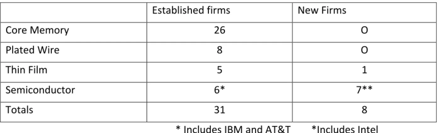
Each of the cases considered above is a highly simplified version of the world. More realistically competition to overturn relatively stable products and markets involves a welter of different alternatives coming from both familiar and unfamiliar sources and origins. Some alternative offerings enjoy increasing investment and commitment, while others drop out of the race or fill a specialized niche. In many cases innovations are put forward by newly formed firms or firms that have newly entered the competition by diversifying from an unexpected direction. An iconic historic example is the race in the computer industry in the 1970s to replace magnetic core memory (Utterback and Brown, 1972). The winner was famously semiconductor memory-‐chips manufactured by Intel, other newly formed firms and by several large incumbents. What is often forgotten is that this race also included a number of plausible alternatives including thin magnetic films and plated wire memories, shown in Table 1. (IBM was advancing both core memory and all three new alternatives; thus there are more entries than firms in column one).
Table 1: Computer Memory Manufacturers in 19701
Established firms New Firms
Core Memory 26 O
Plated Wire 8 O
Thin Film 5 1
Semiconductor 6* 7**
Totals 31 8
* Includes IBM and AT&T *Includes Intel
Today we can see a similar phenomenon in the race between the long established internal combustion engine and electric vehicles (EVs). The contenders in this race include hybrid (combined gasoline and electric) vehicles, battery powered EVs and emerging hydrogen fuel cell EVs. Just to complicate matters within the hybrid category, there are pure hybrids, which run only using an electric motor with a gasoline powered motor and generator; simpler hybrids, which sometimes run electrically and sometimes mechanically; and plug in hybrids recharged occasionally from fixed charging stations and occasionally using an on-‐ board generator. Virtually every large incumbent in the auto industry has introduced their own version of an EV, and virtually all have introduced one or more hybrid vehicles. A handful of newly formed firms have introduced only battery powered electric vehicles. Perhaps hybrid forms of products should be seen as defensive strategies of incumbents alone.
Another assumption we must remove in order to devise a better model of diffusion is the idea that innovations are independent of each other and always in pure competition. Rather, we will argue that modes of interaction among technologies are varied, and that new and older products, at least at the beginning of the diffusion process may experience the expansion of markets for both. If a new competitor causes the market for an established product to grow, sometimes even accelerating its growth, we will, borrowing a term from ecology, call that mode of competition symbiosis. A popular example appears in Mastering
the Dynamics of Innovation (James Utterback, 1994). The first large scale and practical use
of refrigeration began in the early 19th century with tools used to cut blocks of ice from
ponds during the winter and store them in large insulated buildings for use over the summer months. With the development of steam-‐powered machines for freezing blocks of ice, year-‐round ice became a commodity available everywhere on demand. Far from reducing the demand for conveniently harvested ice, mechanical freezing tripled its demand while vastly expanding the use of refrigeration (Utterback, 1994, Chapter 7)!
New and established products in reality almost always influence one another in both positive and negative ways. To borrow another term from ecology, competitors often co-‐ exist as predators and prey, the new products seen as predator and current product as prey. Wolves tend to prey on slower or less able deer and other herbivores, keeping their
1
The table is constructed using data from James M. Utterback and James W. Brown, ”Monitoring for Technological Opportunities,” Business Horizons, October 1972, Vol. 15, 5–15.
population in check. Too small a population of wolves results in overpopulation of herbivores, which then starve for lack of food before the end of winter. Too many wolves may lead to small populations of herbivores and the starvation of wolves. Thus, wolves and herbivores coexist in an oscillating equilibrium with healthy populations of both. Predator-‐ prey competitive modes were extensively examined and modeled (by A. J. Lotka, 1920 and by V. Volterra, 1926). We will build on their work to generalize their idea to the world of
technologies, economics and markets.2 To continue our example, harvested ice and
machine-‐made ice both served ample segments of the market for refrigeration well into the
20th century and well after the appearance of electric refrigeration. Ultimately delivered ice
entered pure competition with electric refrigeration and retreated to small and specialized niches in the market.
In sum, modes of competition need not be unitary, but one mode may evolve into another over time. In general, it is a dynamic process. In the examples we have studied in some detail it is tempting to speculate that we may see symbiosis first; later evolving to a form of predator prey interaction (with either the old or new product dominant for a period of time); followed by the emergence of pure competition with the extinction of one or the other.
The main contributions of this work are the following:
1) We have developed a model for the diffusion of technology not just for head to head competition but also for alternative competitive modes such as predators (N) and prey (M) in equilibrium and in symbiosis.
2) The model provides for analysis of diffusion not simply of one new product (N)
contending with one established product (M), but rather for multiple Mi and Nj.
3) Earlier models such as those presented by Rogers and by Norton and Bass can be readily shown to be special cases of our more general equations.
4) By relaxing the necessity of assuming pure competition, changing modes of competition can be calculated year by year as they evolve.
5) Similarly, by relaxing the need to estimate a total market or niche size in advance, market penetration can be calculated year by year as it evolves.
6) We provide easily used software for analysis, publicly available and updated, in a widely understood simulation language.
7) The model is realistically path dependent providing varying results depending on the starting point of each competition, and this can be represented visually in a phase diagram, at least for the two-‐dimensional M vs. N product case.
8) By using our software and model and analyzing 50 years of data from engineered wood products industry, we show a practical case study of how the “mode” of competition changes in an expected pattern.
Although the term competition is frequently used in the context of innovation and industrial economics an exact description of the term is not usually explicitly given. The interaction between technologies is often not one of competition in the strict sense of the word, as there are many cases where technologies interact in a relationship, which is not necessarily confrontational. The multi-‐mode approach for interaction among technologies provides a useful framework within which to understand and apply this richer landscape of interaction.
Not only do the multiple modes provide the flexibility to examine interaction in the various circumstances where the different technologies inhibit and enhance one another's growth, i.e. in the three distinct modes described below, but it also allows one to account for the transitional effects as the interaction between the technologies transgresses from one mode to another with time. The notion that the modes of interaction between two technologies can change with time is one of the main points that differentiate the technological framework proposed here from similar natural ecological frameworks.
By considering the possibility that one technology may either enhance or inhibit another technology's growth, one finds that three possible modes of interaction can exist, viz. pure
competition where both technologies inhibit the other's growth rate, symbiosis where both
technologies enhance the other's growth rate and predator-‐prey interaction where one technology enhances the other's growth rate but the second inhibits the growth rate of the first. Although such frameworks had, of course, been successfully applied in the fields of biological ecology (Pianka, 1983) and organizational ecology (Brittain and Wholey, 1988) a survey of the literature circa early 1994 showed then that with regard to technologies, pure competition was often discussed, symbiosis sometimes referred to but that predator-‐prey interaction between technologies was very rarely mentioned (Pianka, 1983 in Carroll (Ed.), 1988).
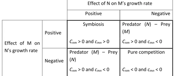
The multi-‐mode framework is illustrated in Figure 1 for the case of two technologies. In principle, the framework can be extended to any finite number of technologies. Note that although there are three modes, two possible predator-‐prey interactions are indicated (depending on which technology is the predator and which the prey), and hence four possible types of interaction. In developing our model in the following section, however, we shall refer to three distinct modes.
Effect of A on B’s growth rate
Positive Negative
Effect of B on A’s growth rate
Positive Symbiosis Predator (A) – Prey (B)
Negative Predator (B) – Prey (A) Pure competition Figure 1: Multi-‐mode framework for the interaction among two technologies
In principle, there are more modes if the cases where one technology has zero impact on the other. For the purpose of our discussion, we can consider those to be special cases, and discuss the interaction with the three modes shown in Table 2.
Once the multi-‐mode framework has been formulated, the next step is to develop a mathematical model. One of the first challenges is to find a metric which defines the concepts of ‘competition’, and ‘good for one another or not’, with mathematical rigor rather than just as qualitative concepts. The concept of growth rate offers itself as a suitable and appropriate way of classifying the process of interaction among technologies, so that in general, interaction can be manifested in the concept of the reciprocal effect that one technology has one another's growth rate.
The following section discusses a mathematical model, which can be used to describe and simulate a framework for multi-‐mode interaction among technologies described in the previous section. In the third section we will present an extended example simulating the
diffusion and interaction of two products over the entire life of a new product from birth to maturity.
Our original contribution here is to present and illustrate the use of a Matlab3 program
based on our model developed by Yilmaz, specifically for modeling the multi-‐mode framework for interaction among technologies. This program has been successfully applied to model the dynamics, and also has the ability to estimate parameters of the LV equations over 50 years by also finding the mode of interactions for the first time.
In the fourth section we will consider strategic and tactical applications of our model and suggest directions for future research.
3 A modified LV system for multi-‐mode interaction among technologies4
Our general model of the diffusion of innovation is based on the Lotka-‐Volterra (LV) equations, originally developed and applied to biological and ecological systems. This section of the paper is based on research conducted by the authors at MIT in early 1994, and draws heavily on a number of papers and conference proceedings in which the work was originally published. The authors presented more details of the mathematical modeling
underpinning the multi-‐mode framework in 1994 (Pistorius and Utterback, 1996).5 A paper
(Pistorius and Utterback, 1995) focused on mortality indicators for mature technologies. The paper setting out the fundamentals of the multi-‐mode framework was published a year later (Pistorius and Utterback, 1997). A number of researchers have since concluded that the LV model exhibits superior performance vis-‐à-‐vis other models.
The concept of substitution inherently implies that two (or more) technologies are competing, and that one is displacing the other. However, traditional substitution models such as the Fisher-‐Pry model, and related but more sophisticated models, presented the dilemma that they did not model two technologies competing against each other, but rather one technology competing against a saturated market or market potential. Due to the fact that a single equation describes the system, the new technology and the rest of the market are coupled in one equation with a few parameters accounting for the adoption of the new technology. Such a formulation yields a solution where the growth of the new technology is accompanied by the decline of the old (given that the size of the market niche stays constant). Single equation formulations do not offer a solution where the older technologies, represented by the market, has a chance of independently “fighting back”. Grübler comments that "... It appears that much of the debate on the appropriate mathematical model(s) of diffusion, in particular the question of symmetrical versus asymmetrical models, may be the result of looking at innovation from a unary (i.e., an innovation grows into a vacuum) or a binary (the market share of an innovation is analyzed
vis-‐a-‐vis the remainder of the competing technologies) perspective. However, diffusion
3 MatLab is a registered trade name. An open source version of our software will soon be available. 4 C.W.I Pistorius, “A growth related, multi-‐mode framework for interaction among technologies”, SM thesis, Alfred P Sloan School of Management, Massachusetts Institute of Technology, 1994. Supervisor: J.M. Utterback. Available at: http://hdl.handle.net/1721.1/12081
5 The paper is also available as an MIT working paper at:
https://www.researchgate.net/profile/James_Utterback/publication/5176207_A_Lotka-‐ Volterra_model_for_multi-‐
mode_technological_interaction__modelling_competition_symbiosis_and_predator_prey_modes/links/543fff ec0cf21227a11ba015.pdf
phenomena generally call for a multivariate approach, which has not yet found wide application in the various diffusion disciplines.” In the general case, one often finds that multiple technologies are vying for market share at the same time and that more than one technology can be growing market share at the same time (Grübler, 1991).
The differential equation(s) describing the diffusion of a technology must be based on the underlying mechanisms involved. In order to model the diffusion characteristics of a technology, it is therefore necessary that the extent of the resources available be taken into account. Finite resources are often embodied in a market niche of finite size. A single equation cannot, however, describe the growth and competition of two technologies simultaneously for it does not account for their respective effects on one another. It can at best model the diffusion of one technology into a market (Carroll, 1981). To model the competition of two technologies, one would need to set up a differential equation for each of the technologies based on the underlying drivers and inhibitors for that technology, together with coupling coefficients that reflect the technologies’ effect on one another’s growth rate. In order to address the problem at hand, it is necessary to model both the technologies explicitly, each with its own equation. They must then be coupled with coupling coefficients to account for the interaction between them.
In order to mathematically model the multi-‐mode framework for interaction among technologies, the traditional and classic substitution models, which are based on single equation formulas, are hence not fit for purpose. It is necessary to model all the technologies, each with its own equation, although they must be coupled with coupling coefficients to account for the interaction between them. A system of coupled differential
equations is therefore required, with each technology represented by its own equation and
coupling between them.
A system that is applicable to this problem (albeit in modified form) was formulated some time ago by the ecologists Lotka and Volterra, known as the Lotka-‐Volterra (LV) equations. Several authors have shown that the Lotka-‐Volterra equations can be successfully applied to model technological diffusion, (among them Bhargava, 1989; Farrell, 1993; Marchetti, 1987; Modis, 1992; Nakićenović, 1979; and as quoted by Marchetti, 1987; and Porter et al., 1991) This is an important observation and we accepted their success as additional justification for pursuing the line of reasoning in the development of this the model. Several authors have shown or commented on the fact that the Lotka-‐Volterra equations can be successfully applied to model technological diffusion. Marchetti, for example, notes that “… I am fairly convinced that the equations Volterra developed for ecological systems are very good descriptors of human affairs. In a nutshell, I suppose that the social system can be reduced to structures that compete in a Darwinian way, their flow and ebb being described by the Volterra equations, the simplest solution of which is a logistic” (Marchetti, 1983).
The reader should take note that the nomenclature Lotka-‐Volterra equations had come to be used to indicate pure competitive as well as predator-‐prey systems, often without explicitly stating which case is being modeled since it is probably assumed that it should be clear from the context. As shown below, the formulations of the Lotka-‐Volterra equations for the different modes are different (specifically regarding the positive/negative sign of the coupling coefficient) and hence have very different characteristics.
In order to understand the fundamentals of the LV system, it is helpful to start with basic logistic growth. The differential equation which underlies this can be expressed as (Girifalco,1991):
!"!" = 𝑎𝑁 − 𝑏𝑁! (1a)
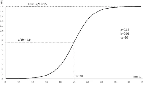
This equation results in the familiar S-‐curve for N(t), shown in Figure 2. It is useful to investigate the physical interpretation of the individual terms in this equation, as it supports the understanding of the modified LV equations for multi-‐mode interaction introduced later.
The first term (aN) fuels exponential growth, where the growth rate at any given time is proportional to the number at that time. Hence the more there are, the faster the growth.
This is shown in equation (1b), where No is a constant indicating the initial condition.
𝑁 𝑡 = 𝑁!𝑒!" (1b)
Very often however, growth is constrained by limited resources. In such an environment, the individual elements vie with one another (competition) for the resources. The vying
interaction is modeled by the term N2. This indicates interaction of elements of the
population with one another, and has a negative effect on the growth rate. The term bN2 is
thus subtracted, or ‘-‐bN2’ added to the equation, to account for this restriction, leading to
the formulation in (1a). In (1b), it is silently assumed that there is no constraint on resources, hence there is assumed to be no vying or competition amongst members of the population so that b=0.
The solution of (1a) is the well-‐known S-‐curve,
𝑁 𝑡 = !!
!!!!(!!!!) (1c)
Figure 2 below shows a typical S-‐curve (with arbitrarily chosen parameters). The upper limit
of growth is a/b and t0 is the time at which the “halfway” mark (i.e. half the value of the
upper limit) is reached. Note how in this case the halfway mark (a/2b=7.5) is reached at
to=50 and the limit (a/b=15) is approached as time progresses.
Figure 2: Typical S-‐curve
3.1 Lotka-‐Volterra equations for ecological systems
The premise of the Lotka-‐Volterra system is that each population (‘species’) is represented by its own equation similar to (1a) in the absence of its interaction with another population. When two or more populations start interacting, a term representing this interaction is then added to each equation.
Consider an ecological system where N represents the predator population and M represents the prey population. In this case, the system of equations representing the dynamics of the total population (N+M) will be (Carroll, 1981):
!"!" = 𝑎!𝑁 − 𝑏!𝑁!+ 𝑐!"𝑁𝑀 (2a) and !" !" = 𝑎!𝑀 − 𝑏!𝑀 ! + 𝑐 !"𝑀𝑁 (2b)
where in this case cnm > 0 and cmn < 0. See also Note 1 regarding conventions pertaining to
the signs of coefficients.
The terms NM and MN indicate elements of the two different species interacting with one
another. In these equations, the terms NM and MN have similar forms and functions as N2
and M2, except that they represent elements of the two different populations interacting
with one another rather than elements of the same interacting with itself.
Equation (2) clearly indicates a predator-‐prey relationship. Since cnm > 0, interaction
between elements of N (predator) and M (prey) will enhance the growth rate of the
predator (N). Similarly, since cmn < 0, interaction between N and M will have a negative
effect on the growth rate of the prey (M).
The nature of ecological populations is such that the cnm and cmn coefficients will always
retain their sign. Mother Nature has mandated that the wolf will always hunt the deer and never the other way around. Hence the relationship between lion and antelope will always be predator-‐prey, with wolf the predator and deer the prey. As we will show, this is not necessarily the case with technologies, where the mode of interaction can change with time, as can the roles of predator and the prey.
For the moment we are also assuming that the coefficients (a,b,c) are constants. However, that does not necessarily have to be so. In the case of technological interaction, it is conceivable that the coefficients may indeed change with time. We return to this issue again later.
3.2 Lotka-‐Volterra equations for multi-‐mode technology interaction
The ecological predator-‐prey equations in Equation (2) can now be modified so they can be used to represent pure competition, symbiosis and predator-‐prey relationships in a formulation to model the multi-‐mode framework for the interaction among technologies. The modification is vested in allowing the signs of the c-‐coefficients to be able to change, and is shown later, for the coefficients to be time dependent rather than constants.
For two technologies, the modified formulation will thus be
and
!"
!" = 𝑎!𝑀 − 𝑏!𝑀! + 𝑐!"𝑀𝑁 (3b)
where the distinction between the different modes is indicated by whether the c-‐ coefficients are positive or negative, as indicated in Table 2. As noted before, c=0 cases can be considered as distinct modes in their own right.
Effect of N on M’s growth rate
Positive Negative
Effect of M on N’s growth rate
Positive
Symbiosis Predator (N) – Prey
(M) Cnm > 0 and cmn > 0 Cnm > 0 and cmn < 0 Negative Predator (M) – Prey (N) Pure competition Cnm > 0 and cmn < 0 Cnm < 0 and cmn < 0
Table 2: Signs of c-‐coefficients in modified LV equations, designating interaction modes
Note 1: The signs of the c-‐coefficients
The authors’ original research and papers (1994-‐1997) used the convention where the
coefficients cnm and cmn were assumed to be always positive, with the distinction
between modes indicated by ± signs preceding the c-‐coefficients. This followed the convention of the original ecological LV equations and supports and intuitive understanding of the LV system. Hence (3b) was originally expressed as
!"
!" = 𝑎!𝑀 − 𝑏!𝑀
! ± 𝑐
!"𝑀𝑁 (3c)
with cmn always positive and the preceding sign (±) indicating the mode (and similarly
for (3a)).
Although there is nothing wrong with this from a convention viewpoint, it later became apparent that a convention where ‘+’ signs precede the c-‐coefficients and the
c-‐coefficients themselves are allowed to be positive or negative has advantages when
programs such as Matlab are used to solve the equations. The programs can then also be used to estimate the coefficients as well as whether they are positive or negative. This is a very powerful concept. Given a data set, the numerical solution will yield not only the intensity of the interaction (numerical value of the coefficients), but also the mode of interaction (reflected in whether the coefficient estimated is positive or negative).
3.3 An iterative solution for the modified Lotka-‐Volterra equations
Although there are several statements in the literature indicating that the Lotka-‐Volterra equations and particularly the pure competition formulation cannot be solved explicitly (see for example Porter, et al, 1991; Hannan and Freeman, 1989), they can be solved numerically. The authors adapted Pielou’s formulation in difference form for the case of pure competition (Pielou,1969). By accounting for the appropriate sign changes (associated with the c-‐coefficients), Pielou's solution for the pure competitive case was then duly
modified to yield solutions for the other modes as well6.
At this point, we revert back to our original convention that c > 0, with the preceding signs explicitly indicated as ‘+’ or ‘-‐’ (see Note 2). For illustrative purposes, this has the advantage of clearly illustrating the mode of interaction.
The modified solution for two technologies in a predator-‐prey mode where N is the predator and M the prey, thus becomes
𝑁 𝑡 + 1 = !!!(!) !!!!! ! ! !!"!! !!!(!) (4a) where 𝛼! = 𝑒!! (4b) 𝛽! = !! !!!! !! (4c) and 𝑀 𝑡 + 1 = !!!(!) !!!!! ! ! !!"!! !!!(!) (5a) where 𝛼! = 𝑒!! (5b) 𝛽! =!!!!!! !! (5c)
Note that difference in signs preceding the third term in the denominators. This determines
N to be the predator and M to be the prey.
3.4 A general solution for multi-‐mode interaction among technologies
Consider now J technologies interacting in the same market niche, and let Ti(t) represent
technology i with (1 ≤ i ≤ J).
The differential equation for Ti(t) can be expressed as
6 Later papers by other researchers also referred to a solution offered by Leslie (Leslie, P.H., “A stochastic model for studying the properties of certain biological systems by numerical methods”, Biometrica, 45 (1957) 16-‐31).
𝑑𝑇𝑖
𝑑𝑡 = 𝑎!𝑇!+ 𝑠!"
!
!!! 𝑐!"𝑇!𝑇! (6)
where all coefficients are positive (see Note 2) and siicii=-‐bi. Furthermore, sij = +1 if
technology j has a positive influence on technology i's growth, whereas sij = -‐1 if technology j
has a negative influence on technology i's growth. Marchetti (1987), Hannan and Freeman (1989) and Modis (1993) among others, have suggested similar sets of equations. However, at the time, they seemed to refer only to the case of pure competition (and not the multiple modes presented here). They did not offer solutions for the equations and specifically not for the multi-‐technology case.
The difference form solution for Ti(t) can be found be extending Pielou's solution to the
general case, i.e.
𝑇!(𝑡 + 1) = !!! !!(!) !! !!"!!" !!!!! !! !!(!) ! !!! (7)
This formulation is a general solution for multi-‐technology, multi-‐mode interaction. It can be used to model the interaction of any finite number of technologies where the interaction
among any pair can either be pure competition, predator-‐prey or symbiosis.7
4 Dynamics of Competitive Modes
Plywood, probably the first wood composite was first produced as a specialty in the late 1800s. Plywood’s value in a wider range of uses became clear during the Second World War, and demand rose rapidly afterward. Production economics and quality depended importantly on the supply of large straight trees with trunks free of knots and defects needed for making veneer. By 1980 the supply of adequate trees had diminished and their price had risen by sixty-‐percent in just five years while quality was in vivid decline. Inferior substitutes for plywood such as wafer-‐board were being tried in some applications. Research by Henry Montrey describes the resulting challenges to the forest-‐products industry and its customers. His masters’ thesis (1982) embodied a deep analysis of both new composite panel options and the plywood panels they might replace in various market segments and new segments. Also covered were technical properties, production processes and economics, and market conditions serving as both incentives and barriers to the adoption of the new composite materials.
A particular experimental composite, made of oriented and layered strands, peeled from widely available smaller trees (Oriented Strand Board, or OSB) was under development. Oriented Strand Board would clearly make more efficient use of a wider variety of forest resources and not just the perfect, large and diminishing old trees required for plywood.
7 The useful application of this formulation has since been overtaken by developments in software packages,
which have the ability to solve complex sets of differential equations. The results below were obtained by Yilmaz. He used the solver algorithms embedded in Matlab (a registered trademark of Mathworks, Inc.) to solve the equations and also to estimate the coefficients and their signs.
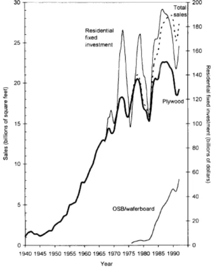
Moreover, the resulting panels were less expensive, stronger and stiffer than plywood of equal thickness making them perfect for use under flooring, roofing and siding, among the major markets for plywood. In 1990 Montrey extended the data from his thesis, compared the early growth of composite panels to the growth of plywood decades earlier, presented the result, and challenged industry leaders to ask why composites would not be at least as successful an innovation. The forecast presented showed expected growth for composites to at least equal the historic early rapid growth of plywood, the industry’s greatest success to date in improving properties and cost (Montrey and Utterback, 1990). Montrey’s forecast helped remove arguments against the consideration of the new panels. In retrospect his analysis, then seen as optimistic, was actually too conservative. It is often easier to see the weaknesses in new ideas judged against current practice, than it is to see their potential strengths and the new values that they alone may offer. His data are shown below with residential fixed investment added. One can see in Figure 3 below that fluctuations in investment fell almost entirely on plywood sales while sales of composite panels grew steadily (Pistorius and Utterback, 1995).
A perplexing question is, ”why, when faced with superior new alternatives, large and long lived competitors resist change?” They are actually often seen to continue investing in and improving older alternating long beyond the point when that makes any economic or strategic sense (Foster, 1986). A pervasive view of competition is to view competition as a zero sum game. We are socialized toward a zero sum view from our earliest experiences with competitive games, the satisfaction of winning and the pain of losing. Who might remember the second pilot to fly alone across the Atlantic Ocean?
In sum, modes of competition need not be unitary, but one mode may evolve into another over time. In general, it is a dynamic process. In the examples we have studied in some detail it is tempting to speculate that we may see symbiosis first; later evolving to a form of predator prey interaction (with either the old or new product dominant for a period of time); followed by the emergence of pure competition with the extinction of one or the other.
Figure 3: U.S. Sales of Plywood and Composite Panels (in constant 1992 Dollars)
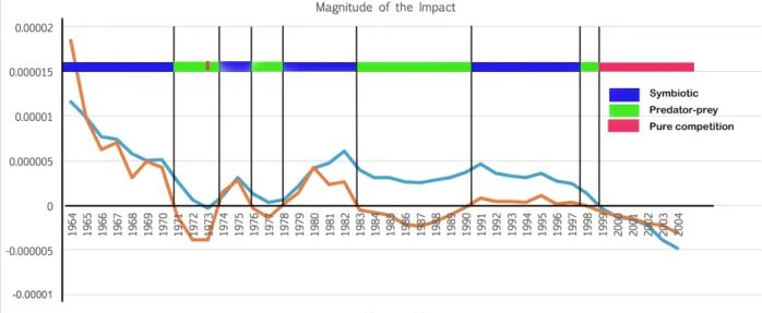
In a provocative new analysis of five decades (1964-‐2014) of sales data in Table 3 and Figure 4 below, Erdem Yilmaz has clearly shown the dynamics of changing modes in this example over time from symbiosis (through 1973) to predator-‐prey (through 1999) and finally competition as expected. This analysis demonstrates the importance of considering the mode of competition in building a scenario. (Each calculation of competitive mode is a decadal average from his simulation). Though this is just a single example from a 50-‐year analysis of the plywood versus OSB competition, it conforms with our hypothesis. We will point below to similar examples such as harvested and machine-‐made ice as precedents.
Table 3: Magnitudes and of modes of competition between OSB and Plywood, 1964-‐20148
In Table 3, “Type of Relationship” shows the mode of interaction between technologies. “Plywood on OSB” is the coefficient representing the impact of decrease or increase of
Plywood’s market size to the one of OSB.9 In columns 3 and 4, blue color represents a
positive impact whereas red color represents a negative impact. Length of the horizontal bars represents the strength of the coefficient. “OSB on Plywood” is the coefficient representing the impact of decrease or increase of OSB’s market size to the one of plywood. “Goodness of fit” is the coefficient representing how well the model matches with the
8 UNECE/FAO TIMBER database, 1964-‐2014
9 The results here are slightly different than those mentioned earlier, as the UNECE/FAO database lumps the diminishing sales of wafer board with those of OSB.
actual data. Length of the horizontal bars represents how well the model matches to the data in the corresponding decade.
Figure 4: Effect of N on M’s growth rate Cnm and M on N’s growth rate Cmn
Figure 4 tells a compelling story. Coefficients of each decade with the indicated starting year are shown. Plywood’s impact on OSB is shown in blue color and OSB’s impact on plywood is shown with red. The relationship (“mode of interaction”) is evident from the sign of the coefficient. In the early years, we observe that the magnitude of interaction is at its peak compared to the following years. The magnitude of the impact is observed to shrink over the years.
The results are impressive. Not only as they apply to this specific case, but in general showing how the interaction modes change over time. Many researchers (including ourselves) have postulated that this happens, but we cannot recall having come across similar results – based on data -‐ which show the dynamic nature of the relationship, with the interaction changing from symbiosis to predator-‐prey to pure competition as time evolves. The underlying issue here is that the coefficients change with time – most of the models just assume that the coefficients are constants. The fact that the coefficients change with time has significant implications for application in innovation strategy.
Prior reports have observed oscillations in market share during product competitions (including Marchetti, 1983; Modis and Debecker, 1992; and Modis, 1992, 1993) and have suggested that the fluctuations become random or chaotic when populations or markets approach saturation. Montrey and Utterback, (Montrey and Utterback 1990) suggest that oscillations may indicate the emergence of a new technology and the demise of the old. Referring to the oscillations in the mature phase of plywood’s growth they state, “we venture to hypothesize that the type of variance in the production of a commodity such as shown for plywood in recent years… is a clear sign of the vulnerability of the product to an emerging substitution.” In the case of OSB and plywood we have one can observe that the oscillations of sales of plywood shown in Figure 3 seem to match fluctuations in residential fixed investment. Comparing Figure 3 with figure 4 one can see that each time construction