• Aucun résultat trouvé

Regularization schemes for transfer learning with convolutional networks

N/A
N/A
Protected

Academic year: 2021

Partager "Regularization schemes for transfer learning with convolutional networks"

Copied!
131
0
0

Texte intégral

(1)

HAL Id: tel-02439193

https://tel.archives-ouvertes.fr/tel-02439193

Submitted on 14 Jan 2020

HAL is a multi-disciplinary open access archive for the deposit and dissemination of sci-entific research documents, whether they are pub-lished or not. The documents may come from teaching and research institutions in France or abroad, or from public or private research centers.

L’archive ouverte pluridisciplinaire HAL, est destinée au dépôt et à la diffusion de documents scientifiques de niveau recherche, publiés ou non, émanant des établissements d’enseignement et de recherche français ou étrangers, des laboratoires publics ou privés.

convolutional networks

Xuhong Li

To cite this version:

Xuhong Li. Regularization schemes for transfer learning with convolutional networks. Technology for Human Learning. Université de Technologie de Compiègne, 2019. English. �NNT : 2019COMP2497�. �tel-02439193�

(2)

Par Xuhong LI

Thèse présentée

pour l’obtention du grade

de Docteur de l’UTC

Regularization schemes for transfer learning with

convolutional networks

Soutenue le 10 septembre 2019

Spécialité : Informatique : Unité de recherche Heudyasic

(3)

THESIS  Submitted in partial fulfillment of the requirements  for the degree of Doctor 

Spécialité : Informatique 

Area of specialization: Computer Science  by 

X

UHONG 

L

        Regularization Schemes for Transfer Learning with    

Convolutional Networks 

10/09/2019  Heudiasyc Laboratory, UMR UTC/CNRS 7253  Thesis Committee: 

Rapporteurs  Nicolas Thome  Professor CNAM CEDRIC Lab 

  Gilles Gasso  Professor INSA Rouen 

Examinateurs  Elisa Fromont  Professor Université Rennes 1    Alain Rakotomamonjy  Professor Université de Rouen 

  Véronique Cherfaoui  Professor Université de technologie de  Compiègne 

Directeurs  Yves Grandvalet  CNRS senior researcher 

  Franck Davoine  CNRS researcher 

(4)

First and foremost, I would like to express my gratitude to my supervisors of the thesis, Yves Grandvalet and Franck Davoine, for their continuous support of my PhD life, for their patience, motivation, and immense knowledge. Franck and Yves have taught me the way of thinking and researching as professional researcher, the tenacity of perfecting a job, as well as the professional knowledge in the field of statistics, machine learning and computer vision. I appreciate every discussion, meeting with them that gave me the motivation to keep working on challenging problems. I am grateful for their wise guidance throughout my thesis, and I feel so lucky to work under their supervision.

I would like to thank the committee members for joining my defense of the thesis. Many thanks to Nicolas Thome and Gilles Gasso for reviewing my manuscript during the summer vacation, and to Elisa Fromont, Alain Rakotomamonjy and Véronique Cherfaoui for all their comments and insightful suggestions for improving the thesis.

I also want to thank the Chinese Scholarship Council (CSC) from Chinese govern-ment for the financing during my PhD, and Heudiasyc laboratory, UMR UTC/CNRS 7253 for supporting me to participate in international conferences, and for buying the powerful GPU servers at the beginning of my thesis that makes it possible for me to finish my experiments.

I warmly thank my labmates of Heudiasyc, whose friendships made me have a memorable experience at UTC. I also appreciate my dear Chinese friends for their help and encouragement. I could not have smoothly survived from the PhD thesis without their accompanying. I would like to give my sincere thanks to my parents for their unconditional love and support.

Last but not least, I thank Xiaolei, my best friend and my wife, for understanding me and helping me throughout these years with all her efforts.

(5)
(6)

Transfer learning with deep convolutional neural networks significantly reduces the computation and data overhead of the training process and boosts the perfor-mance on the target task, compared to training from scratch. However, transfer learn-ing with a deep network may cause the model to forget the knowledge acquired when learning the source task, leading to the so-called catastrophic forgetting. Since the efficiency of transfer learning derives from the knowledge acquired on the source task, this knowledge should be preserved during transfer. This thesis solves this prob-lem of forgetting by proposing two regularization schemes that preserve the knowl-edge during transfer. First we investigate several forms of parameter regularization, all of which explicitly promote the similarity of the final solution with the initial model, based on the L1, L2, and Group-Lasso penalties. We also propose the variants that use Fisher information as a metric for measuring the importance of parameters. We validate these parameter regularization approaches on various tasks. The second reg-ularization scheme is based on the theory of optimal transport, which enables to es-timate the dissimilarity between two distributions. We benefit from optimal transport to penalize the deviations of high-level representations between the source and target task, with the same objective of preserving knowledge during transfer learning. With a mild increase in computation time during training, this novel regularization approach improves the performance of the target tasks, and yields higher accuracy on image classification tasks compared to parameter regularization approaches.

Keywords —

transfer learning, regularization, convolutional networks, optimal transport, computer vision.

(7)
(8)

L’apprentissage par transfert de réseaux profonds réduit considérablement les coûts en temps de calcul et en données du processus d’entraînement des réseaux et améliore largement les performances de la tâche cible par rapport à l’apprentissage à partir de zéro. Cependant, l’apprentissage par transfert d’un réseau profond peut provoquer un oubli des connaissances acquises lors de l’apprentissage de la tâche source. Puisque l’efficacité de l’apprentissage par transfert vient des connaissances acquises sur la tâche source, ces connaissances doivent être préservées pendant le transfert. Cette thèse résout ce problème d’oubli en proposant deux schémas de régularisation préser-vant les connaissances pendant l’apprentissage par transfert. Nous examinons d’abord plusieurs formes de régularisation des paramètres qui favorisent toutes explicitement la similarité de la solution finale avec le modèle initial, par exemple, L1, L2, et Group-Lasso. Nous proposons également les variantes qui utilisent l’information de Fisher comme métrique pour mesurer l’importance des paramètres. Nous validons ces ap-proches de régularisation des paramètres sur différentes tâches de segmentation sé-mantique d’image ou de calcul de flot optique. Le second schéma de régularisa-tion est basé sur la théorie du transport optimal qui permet d’estimer la dissimilar-ité entre deux distributions. Nous nous appuyons sur la théorie du transport opti-mal pour pénaliser les déviations des représentations de haut niveau entre la tâche source et la tâche cible, avec le même objectif de préserver les connaissances pen-dant l’apprentissage par transfert. Au prix d’une légère augmentation du temps de calcul pendant l’apprentissage, cette nouvelle approche de régularisation améliore les performances des tâches cibles et offre une plus grande précision dans les tâches de classification d’images par rapport aux approches de régularisation des paramètres.

Keywords —

apprentissage par transfert, régularisation, réseaux de neurones à convolution, transport optimal, vision par ordinateur.

(9)
(10)

Contents 1

List of Figures 5

List of Tables 7

List of Algorithms 9

1 Introduction 11

1.1 Context and Motivation . . . 11

1.2 Contributions and Thesis Outline . . . 13

1.3 Terminology . . . 14

2 Background and Related Work 17 2.1 Convolutional Neural Networks . . . 18

2.1.1 Elemental Units in Convolutional Networks . . . 18

2.1.2 Optimization Algorithms of Deep Networks . . . 21

2.1.3 Recent Advances in Convolutional Neural Network Structures 23 2.1.4 Fully Convolutionalizing the Network . . . 25

2.1.5 Structure Modifications for Image Segmentation . . . 27

2.1.6 Structure Modifications for Other Vision Tasks . . . 31

2.2 Transfer Learning . . . 33

2.2.1 Domain Adaptation . . . 34

2.2.2 Multi-Task Learning . . . 35

2.2.3 Lifelong Learning (Continual Learning) . . . 35

2.2.4 Inductive Transfer Learning with CNN . . . 36

2.3 Optimal Transport . . . 37

(11)

2.3.2 Entropic Solvers . . . 39

2.3.3 Optimal Transport Applications in Deep Learning. . . 40

2.3.4 Optimal Transport on Neuron Distributions . . . 42

2.4 Regularization Approaches . . . 42

2.4.1 Regularizers Bringing Desirable Properties . . . 43

2.4.2 Regularizers Creating Synthetic Training Examples . . . 44

2.4.3 Regularizers with Good Randomness . . . 44

2.4.4 Regularizers as Inductive Bias for Better Learning . . . 45

3 Parameter Regularizers for Fine-Tuning 47 3.1 Introduction . . . 48

3.2 Related Work . . . 51

3.3 -SPRegularizers . . . 52

3.4 Experimental Results in Image Classification . . . 55

3.4.1 Source and Target Databases . . . 55

3.4.2 Training Details. . . 56

3.4.3 Comparison across Penalties, Source and Target Databases . . 57

3.4.4 Fine-Tuning from A Similar Source . . . 58

3.5 Analyses. . . 60

3.5.1 Behavior on the Source Task . . . 61

3.5.2 Fine-Tuning vs. Freezing the Network . . . 61

3.5.3 Layer-Wise Analysis . . . 63

3.5.4 Computational Efficiency . . . 64

3.5.5 Theoretical Insights. . . 65

3.6 Other Setups. . . 67

3.6.1 Transfer Learning Approaches . . . 68

3.6.2 Experimental Setup . . . 70

3.6.3 Experimental Results . . . 74

3.6.4 Analysis and Discussion . . . 79

3.7 Conclusion . . . 79

4 Representation Regularizers for Fine-Tuning 81 4.1 Introduction . . . 82

4.2 Related Work . . . 84

4.3 A Reminder on the Optimal Transport Problem and the Sinkhorn Solvers 85 4.4 Representation Regularizers . . . 86

(12)

4.4.1 Representation Regularization via Optimal Transport . . . 86

4.4.2 Two Baselines . . . 87

4.5 Experimental Results . . . 89

4.5.1 Datasets . . . 89

4.5.2 Experimental Details . . . 89

4.5.3 Comparison across Regularizers . . . 90

4.6 Analyses and Discussions . . . 91

4.6.1 Comparison with Transporting Data . . . 91

4.6.2 Possible Transport . . . 92

4.6.3 Effective Transport . . . 94

4.6.4 The Envelope Theorem . . . 95

4.7 Other Regularizers Tested. . . 96

4.8 Conclusion . . . 97

5 Contributions and Perspectives 99 5.1 Contributions . . . 99

5.2 Perspectives . . . 101

Publications 105

(13)
(14)

1.1 Illustration of a neuron and an activation . . . 14

2.1 Illustration of a simple convolutional network . . . 19

2.2 Comparison between a simple convolutional network and a fully con-volutionalized network . . . 26

2.3 Illustration of a fully convolutionalized network . . . 28

2.4 Illustration of a fully convolutional network proposed by Long et al. [2015a] . . . 30

2.5 Illustration of the atrous spatial pyramid pooling (ASPP) module pro-posed by Chen et al. [2018a] . . . 30

2.6 Illustration of the pooling pyramid module proposed by Zhao et al. [2017] . . . 31

3.1 Illustration of the inadequacy of the standard L2 regularization in transfer learning . . . 50

3.2 Classification accuracy (in %) on Stanford Dogs 120 for L2-SP . . . . 56

3.3 Classification accuracies (in %) of the tested fine-tuning approaches on the four target databases . . . 59

3.4 Classification accuracies of fine-tuning with L2 and L2-SP on Stan-ford Dogs 120 and Caltech 256–30 when freezing the first layers of ResNet-101 . . . 62

3.5 R2 coefficients of determination with L2 and L2-SP regularizations

for Stanford Dogs 120 . . . 64

3.6 Boxplots of the diagonal elements of the Fisher information matrix computed on the training set of ImageNet using the pre-trained model 65

4.1 Traces of the optimal transport plans at the output of each ResNet-101 unit . . . 93

(15)

4.2 Traces of the optimal transport plans at the penultimate layer during training . . . 94

(16)

3.1 Characteristics of the target databases: name and type, numbers of

training and test images per class, and number of classes. . . 56

3.2 Average classification accuracies (in %) of L2, L2-SP and L2 -SP-Fisheron 5 different runs . . . 60

3.3 Classification accuracy drops on the source tasks due to fine-tuning based on L2, L2-SPand L2-SP-Fisherregularizers. . . 63

3.4 Training and test details for segmentation on Cityscapes . . . 70

3.5 Source datasets for transfer learning . . . 72

3.6 Target datasets for transfer learning . . . 72

3.7 Summary of experimental results . . . 75

3.8 EncNet pixel accuracy and mIoU on the PASCAL Context validation set according to regularization hyper-parameters. . . 76

3.9 Average endpoint errors on the two subsets of the Scene Flow dataset 77 3.10 DSTL classification accuracy using the Inception-V3 network on the Birds200 validation set according to regularization hyper-parameters. 78 4.1 Average classification precision of no-regularized, L2, L2-SP, ΩI, ΩR and ΩP using ten-crop test . . . 91

(17)
(18)

1 A direct implementation of convolution in the l-th layer . . . 20

2 Stochastic gradient descent (SGD) update at training iteration k . . . . 22

(19)
(20)

Introduction

Contents

1.1 Context and Motivation . . . 11

1.2 Contributions and Thesis Outline . . . 13

1.3 Terminology . . . 14

1.1

Context and Motivation

Deep neural networks have been applied to fields including computer vision, natural language processing, speech recognition, machine translation as well as board game programs, where they have produced results comparable to and in some cases supe-rior to human experts. These deep network models contain millions of parameters to be estimated and require billions of operations for a single forward pass, leading to an obligation of enormous computation resources for fast experimental evaluations, numerous training data for assuring the desired performance, and a delicate design of network structures together with a good initialization of parameters for the gradient-based optimization. Facing these problems, it is not practical for each single task to collect a lot of training data, or spend weeks or months on searching the best train-ing scheme. Few companies and laboratories are capable of launchtrain-ing such costly experiments.

Transfer learningcan yet relieve the pain. The idea of transfer learning is to gain prior knowledge from solving a source task, and to exploit the stored knowledge to solve a different but related target task. Fortunately, the open-source environment in

(21)

this community encourages the release of large-scale datasets and pre-trained deep network models, which boosts a lot the research in the community. During trans-fer learning, some form of knowledge that is learned from the source task is then transferred to the target task and exploited to improve the performance. Technically, fine-tuning, a common tool for transferring knowledge, initializes the model with the pre-trained parameter values, and continues training on the target dataset for adaption to an optimal solution for the target task. Through fine-tuning and transfer learn-ing, the training process can be largely shortened to hours or minutes, and less prone to overfitting when there are few data available on the target task. However, trans-fer learning with deep networks may cause the model to easily forget the knowledge learned from the source, leading to the known catastrophic forgetting. Since the effi-ciency of transfer learning derives from the learned knowledge in the source task, the knowledge should be preserved during transfer learning, especially when the source task is “rich” and contains a large-scale dataset.

This thesis thus proposes approaches for preserving the knowledge during transfer learning. We propose to implement this inductive bias of preserving the source knowl-edge for transfer learning problems through regularization approaches. In most cases of machine learning, data are split into training set and test set, which are used for training the model and measuring the performance of the learned model respectively. Regularization approaches are designed, via various ways, to reduce the test error, i.e. the error that the learned model makes on the test data set, sometimes at the expense of the increased error on the training data set. The regularization approaches are applied during the training phase and hence cause increased computation during training, but no additional operations for inference during testing. In addition, the increased com-putation during training is usually mild compared to the comcom-putation of the input data passing through the deep network.

Many regularization approaches are actually motivated by an inductive bias to-wards a desired model or a preferred property in the learned model, and, as we dis-cussed before, the desired one in this thesis is to maximally preserve the knowledge from the source task. In terms of knowledge, we propose two points of view:

• If two models with the same structure have similar parameters, then they contain similar knowledge.

• If for any input, two models always yield similar outputs, then they contain similar knowledge.

(22)

The first point of view may need delicacy on the definition of similar parameters, since each parameter is in different scale for the contribution of the model’s discrimination capacity. We tackle this problem via the Fisher information matrix, and compare with simply ignoring it, and find that in practice, the different scales for parameters are not so bothersome. The second point view also needs some concrete definitions on the similar outputs. We consider measuring the outputs at the penultimate layer of a deep network, as they can be seen as the most advanced features extracted by the network for the discrimination layer.

Thereby, we propose to transfer the knowledge through parameters and representa-tions, based on which we respectively propose two different families of regularization approaches in this thesis. While the proposed regularization approaches can be ap-plied widely in many transfer learning problems, we evaluate them under a particular and practical setting in transfer learning, where a vast amount of data was available for training on the source problem, and some limited amount of labeled data is avail-able for solving the target problem. Note that different from the setting we consider, many applications like domain adaptation, network compression, lifelong learning, reinforcement learning, where knowledge can be accumulated, may also benefit from our proposed regularization approaches.

1.2

Contributions and Thesis Outline

Following the motivations and the propositions, this thesis is simply organized as fol-lows:

In Chapter2, we present the background concepts. First we introduce the convo-lutional neural networks, including the unit operations, optimization algorithms and recent advances in computer vision. Then we recall the transfer learning definition and categorization, and discuss the applications of convolutional networks in transfer learning. After that, we introduce a mathematical tool of measuring the distance be-tween two probability distributions, the optimal transport theory, which is exploited to preserve the source knowledge during transfer learning and based on which we develop the regularization approach on representations. At the end of Chapter 2, we give a general introduction on the regularization approaches in deep learning and some thoughts about using regularization as inductive bias for better learning.

In Chapter3, we present the regularization approaches that are based on parame-ters for transfer learning with convolutional networks. We show that they all encode an

(23)

Σ ϕ 1 x0 x1 x2 xn b w 0 w1 w2 wn .. . y = ϕ(Pn i=0xiwi+ b)

Figure 1.1: Illustration of a neuron and an activation. ϕ is the activation function, b is the bias, and the output y can be also referred as activation or activity.

explicit bias towards the pre-trained parameters learned on the source task, preserving the source knowledge. We validate the parameter regularization approaches on vari-ous experiments in image classification, image segmentation, video segmentation and optical flow estimation. Analyses and theoretical hints are also provided.

In Chapter4, instead of focusing on the parameters, we propose a novel regular-ization approach based on the optimal transport theory to penalize the deviations of the output activations on the target task, with the same objective of preserving the knowledge during transfer learning. We show that this novel regularization approach also improves the performance of the target tasks, and yields higher accuracy on image classification tasks than parameter regularization approaches.

In Chapter 5, we conclude the thesis, summarize our contributions and suggest some possible paths to future research.

1.3

Terminology

Before opening this thesis, we would like to clarify some terms in context of machine learning and artificial neural networks.

Neurons, Activations In context of artificial neural networks, an artificial neuron, or simply a neuron, is a mathematical function conceived as a model of biological neurons. It consists in two functions, a weighted sum of inputs, and a non-linear acti-vation functionthrough which the sum is passed. The output of a neuron is sometimes referred as activation or activity. Mathematically, a neuron is a function with opera-tions and parameters while an activation is an output value of the neuron, see Figure

(24)

Channels, Kernels, Filters Regarding convolutional neural networks where the in-put is usually an image with RGB color channels, activations at a hidden layer com-pose a feature map, i.e. a 3D tensor with the height, the width and the number of channels. In computer vision, particularly image processing, a kernel is a convolution matrix yet without trainable parameters, used for blurring, sharpening, edge detection and other filters. So sometimes, a kernel can be referred as a filter, especially in the field of signal processing. A convolutional kernel in convolutional networks has no difference from the conventional kernel except that the values in the convolutional kernel can be trainable by machine learning algorithms. Usually, the convolution be-tween a kernel and an image produces a channel. So the number of channels at a layer is equal to the number of kernels. Thereby, we do not much distinguish the three notions in this thesis: channels, kernels, filters, regardless of their subtle difference.

Features, Representations, Activations In pattern recognition, extracting pertinent features of the data is a crucial step for effective learning algorithms. Traditionally, this step is manually done by feature engineering, but feature learning or represen-tation learning proposes to replace feature engineering by allowing the machine to both learn the features and use them to perform a specific task. Because of this fea-ture/representation learning scheme, representations also refer to features. Features or representations are slightly different from the activations as the activations denote the evaluation of features or representations on particular instances. We respect this difference throughout the thesis.

Parameters, Weights In general, parameters and weights are both trainable vari-ables, embedded in a function. Depending on the variable values, this function can cause different effects and extract different features from the data. Learning algo-rithms search for the optimal values for these parameters and weights. In neural net-works, weights specifically refer to the variables that are multiplied by the inputs of the current layer, and there is an extra variable that is simply multiplied by 1. This extra variable is also trainable and named bias. All the weights and biases are the trainable parameters in the neural network.

(25)
(26)

Background and Related Work

Contents

2.1 Convolutional Neural Networks . . . 18

2.1.1 Elemental Units in Convolutional Networks . . . 18

2.1.2 Optimization Algorithms of Deep Networks. . . 21

2.1.3 Recent Advances in Convolutional Neural Network Struc-tures. . . 23

2.1.4 Fully Convolutionalizing the Network . . . 25

2.1.5 Structure Modifications for Image Segmentation . . . 27

2.1.6 Structure Modifications for Other Vision Tasks . . . 31

2.2 Transfer Learning . . . 33

2.2.1 Domain Adaptation. . . 34

2.2.2 Multi-Task Learning . . . 35

2.2.3 Lifelong Learning (Continual Learning) . . . 35

2.2.4 Inductive Transfer Learning with CNN . . . 36

2.3 Optimal Transport . . . 37

2.3.1 Mathematical Definition . . . 38

2.3.2 Entropic Solvers . . . 39

2.3.3 Optimal Transport Applications in Deep Learning. . . 40

2.3.4 Optimal Transport on Neuron Distributions . . . 42

(27)

2.4.1 Regularizers Bringing Desirable Properties . . . 43

2.4.2 Regularizers Creating Synthetic Training Examples . . . . 44

2.4.3 Regularizers with Good Randomness . . . 44

2.4.4 Regularizers as Inductive Bias for Better Learning . . . . 45

Prologue In this chapter, we present the background concepts. First we introduce the convolutional neural networks, including the unit compositions of the network, the evolution of network structures, and recent advances of convolutional networks in computer vision. Then we recall the transfer learning definition and categorization, and discuss the applications of convolutional networks in transfer learning. After that, we introduce a mathematical tool of measuring the distance between two probability distributions, the optimal transport theory, which will be used to develop a regular-ization approach for preserving the source knowledge during transfer learning. At the end of this chapter, we give a general introduction on the regularization approaches in deep learning and some thoughts about using regularization as inductive bias for better learning.

2.1

Convolutional Neural Networks

Convolutional neural networks have their first success in the 1980s [LeCun et al.,

1989] for recognizing handwritten digits from small binarized images. The network used at that time is LeNet [LeCun et al.,1989], a very small convolutional network, but inspires the invention of the first modern convolutional network AlexNet [Krizhevsky et al., 2012], which has won the ImageNet large-scale visual recognition competition [Deng et al.,2009] in 2012 by a wide margin over other models.

2.1.1

Elemental Units in Convolutional Networks

Convolution and Feature Maps The essential operation in convolutional neural network is, without question, the convolution. Algorithm 1 presents a direct imple-mentation of convolution for better understanding the convolution operation, without forgetting that it can be largely sped up by parallel computing. With other elemental units, Figure 2.1 shows a simple convolutional neural network for image classifica-tion. In this thesis, we consider the notion of layers as the sets of activations or the

(28)

input image layer l = 0 convolutional layer layer l = 1 convolutional layer layer l = 2 convolutional layer layer l = 3 convolutional layer layer l = 4

fully connected layer layer l = 5

output layer l = 6

Figure 2.1: An illustration of a simple convolutional network with a single-channel image as input.

outputs of neurons, which are determined real values, distinguished from trainable parameters. Note that there are no parameters at layer 0. The slices in black in con-volutional layers and the sticks in fully connected layers are the activations or called the feature maps in convolutional networks. The small (sliding) windows with colors present the convolutional kernels where the parameters reside. Each of these windows does an element-wise multiplication of kernel parameters and activations within the window, a sum of all the resulted elements, and a non-linear activation function. This operation will be repeated when these windows, with the same parameters, slide onto a new position of the image plane or the feature map plane. As for fully connected layers, all activations are fully connected to those in the previous layer.

Each feature map (or the set of activations in the feature map plan) A in a con-volutional layer is a 3D tensor of dimension W × H × Cout, and computed by a 4D

tensor k of Cin× Cout× k × k, which is named as convolutional kernel, where Cinis

the number of feature map slices in the previous layer, Cout is the number of feature

map slices in this layer, and k × k is the window size, varying from 1×1 to 7×7. The size of kernel can be set arbitrarily and it controls principally the size of the network. It can be set very large to have enough capacity of the model being representative and yet be prone to overfitting, or it can be very small for speeding up the training and test phrases. For balancing the representative capacity and the risk of overfitting, and also following the practical engineering advice (related to the GPU memory and computa-tion speed), the sizes of convolucomputa-tion kernels always start with a small value in the first layers and then increase gradually along the network with the dimensions of feature

(29)

Algorithm 1 A direct implementation of convolution in the l-th layer

1: for cout in 1...Coutdo

2: for w in 1...W do 3: for h in 1...H do 4: for x in 1...k do 5: for y in 1...k do 6: for cinin 1...Cin do 7: Al[w, h, cout] + = Al−1[w + x, h + y, cin] × k[cin, cout, x, y] 8: end for 9: end for 10: end for 11: end for 12: end for 13: end for maps decreasing.

The convolution operation enables the parameter sharing and the translation invari-ance properties. For each position of the feature map, the same parameters are used for extracting the features, as the kernel window slides on the feature map plan. In a traditional neural network, each element of the parameter matrix is used exactly once when extracting the features. The property of sharing parameter thus reduces largely the number of trainable parameters. As for the translation invariance, the convolution helps to detect the translated features. When the input image is translated, the features related to the objects change positions but will still be captured as the convolution kernel slides on the feature plan, and these important features will be given to the next layer and contribute for the discrimination.

Non-Linear Activation Functions Besides the convolution operation, non-linear activation functions are another important component in (convolutional) neural net-works, and the stack of activation functions in neural networks can help the network to learn complex data, approximate almost any function representing a feature, and provide accurate predictions. Non-linear activation functions are usually simple and computationally efficient. Several choices are preferred in the community, like tanh, sigmoid , ReLU (rectified linear unit ), etc. For deep convolutional neural networks,

(30)

ReLU is a desirable choice among many activation functions for its efficacy and not easily falling into the gradient diminishing problem.

Pooling Pooling is an operation once frequently used in convolutional neural net-works, but for modern convolutional netnet-works, pooling layers are replaced by convo-lution layers with an equivalent stride, while a pooling layer is applied before the last layer for reducing the feature map spatial dimensions by averaging all outputs of each feature map.

2.1.2

Optimization Algorithms of Deep Networks

A learning problem is different from a pure optimization problem. In most machine learning scenarios, we have no access to the true data distribution noted as pdata,

caus-ing the pure optimization problem unfeasible. Instead, a learncaus-ing problem exploits an optimization algorithm to minimize a loss function with respect to the empirical distri-bution, i.e. the training data set, noted as ˆpdata, hoping the optimized model performs

well with respect to pdata, or a related test data set. Throughout this thesis, we develop

the supervised case, where the per-example loss function L is related to the output of the model f (x; w) and the label y. Then the generalization loss or error J∗(w), which measures the performance of the learned model, is the expectation of the per-example loss over the true underlying distribution pdata:

J∗(w) = E(x,y)∼pdataL(f (x; w), y). (2.1)

Since this data generating distribution pdata is difficult to access, we cannot directly

compute the generalization error. The simplest solution is to minimize the expected loss on the training set ˆpdata:

J (w) = E(x,y)∼ ˆpdataL(f (x; w), y). (2.2)

Specifically, this expectation can be obtained by the average over all training exam-ples: E(x,y)∼ ˆpdataL(f (x; w), y) = 1 N N X i=1 L(f (xi; w), yi), (2.3)

where N is the number of training examples. Then the learning problem is to search an optimal solution of Equation 2.3 with an optimization algorithm, expecting the solution, i.e. the learned model, to have small generalization error. In practice, the

(31)

Algorithm 2 Stochastic gradient descent (SGD) update at training iteration k

1: Require Learning rate (k), parameters w(k), mini-batch size m

2: while stopping criterion not met do

3: Sample a mini-batch of m examples from the training set {xi} with

corre-sponding targets {yi}. 4: Compute gradients: g(k)← ∇ wm1 Pm i=1L(f (xi; w(k)), yi) 5: Update parameters: w(k+1)← w(k)− (k)g(k) 6: end while

algorithms that are used for deep learning are based on stochastic gradient descent, which is slightly different from solving the Equation 2.3. The SGD algorithm is an iterative gradient-based algorithm. In each iteration, the algorithm randomly selects a mini-batch of training examples, to evaluate the gradients of the loss function with re-spect to the parameters, then update the parameters by a small step of the gradients for minimizing the loss function, and it stops until the stopping criterion is met. Updat-ing parameters through the SGD algorithm is presented in Algorithm2. More details about the practical and intuitive views of using SGD for optimizing deep networks can be found in [Goodfellow et al.,2017, Section 8.1.2 and 8.1.3].

The SGD algorithm has many variants, including SGD with momentum, SGD with Nesterov momentum [Nesterov, 1983; Sutskever et al., 2013], Adagrad [Duchi et al.,2011], RMSprop [Tieleman and Hinton,2012], Adam[Kingma and Ba,2015], to name a few. They are all based on gradients and the difference is the way of updating parameters. We refer the interested readers to Ruder[2016] for the introduction and the motivation of each SGD variant.

An open question still remains about the SGD algorithms. When optimizing a con-vex function, a minimum is always good because any local minimum is guaranteed to be a global minimum. However, with non-convex functions, such as neural networks, it is possible to have many local minima and we are not sure about these minima. Whether SGD and its variants encounter these local minima and whether these local minima have high generalization error, it still remains an open question in the commu-nity. However, experts now suspect that, for sufficiently large neural networks, most local minima have a low generalization error value, and that it is not important to find a true global minimum rather than to find a point in parameter space that has low but not minimal cost [Goodfellow et al., 2017, Section 8.2.2]. This can be done with the SGD algorithms. So in this thesis, we continue to apply the SGD with momentum to

(32)

train the convolutional networks.

2.1.3

Recent Advances in Convolutional Neural Network

Struc-tures

LeNet and AlexNet are two networks aforementioned, their structures are very simple, starting with several convolutional layers and ending with two or three fully connected layers. This simple design is yet inefficient. In this subsection, we briefly review the problems of this simple design and discuss the advances in neural network structures, including the general designs and the partial components. Since AlexNet, the research on network structure has been wildly explored.

Receptive Field The receptive field of a good network was suggested to be large enough to cover the whole image to capture the global information. Five convolutional layers in AlexNet are far away from enough to get a large receptive filed. Simonyan and Zisserman[2015] showed that the sequence of two convolutional layers of kernel size 3 × 3 is equal to one layer of 5 × 5 but has less parameters, so they encouraged to use more 3 × 3 layers instead of one large layer. Based on this idea, Simonyan and Zisserman[2015] proposed a 19-layer network VGG with the same network de-sign (several straightforward convolutional plus three fully connected layers). The “theoretical” receptive field is not widely applicable and sometimes inexplicable for some problems, e.g. image segmentation. Despite that this is still an open question, the network VGG is powerful and popular, also robust when applying on the transfer learning problems.

Deeper or Wider Second, rather than going deeper,Szegedy et al.[2015] concate-nated four convolutional layers of different sizes and proposed Inception network (also called GoogLeNet). Instead of choosing a best kernel size, or stacking 3 × 3 layers,

Szegedy et al. [2015] decided to have them all. Moreover, in each block, to avoid the extra parameters when using large size kernels,Szegedy et al.[2015] followed the suggestion in Lin et al.[2014a], i.e., inserting a layer of 1 × 1 to reduce the number of slices before the convolution of 3 × 3 or 5 × 5. This network has a depth of 22 with some width. Inception networks also follow some engineering insights. If all the layers are sequential, the computation of forward and backward cannot move to the next layer before finishing all the computations at the current layer, wasting time to

(33)

wait all threads to be finished in the parallel algorithm. In addition, small convolution operations may not occupy all processing units but large ones may need more, leading some processing units free at some moments. So a good engineer design of the several parallel convolutions is possible to make good use of the powerful parallel resources.

Batch Normalization When there are more layers between the input and output, the vanishing gradient problem becomes more critical. Since activation functions like sigmoid, tanh or ReLU, have the gradients in range between 0 and 1, the gradients computed by the chain rule vanish exponentially backwards. Therefore, it happens easily for deep networks that gradients in the first layers are very small and have little or none effect when updating the parameters. For solving this vanishing gradient problem, Ioffe and Szegedy [2015] proposed to achieve a standard normal distribution for each layer by normalizing the inputs via mini-batch statistics. This new mechanism is called batch normalization, and integrated into later versions of Inception networks [Ioffe and Szegedy,2015;Szegedy et al.,2016, 2017], as well as many other networks. In practice, batch normalization accelerates the training process, makes the parameter initialization less important, and improves the performance. We will continue to discuss batch normalization later in Section2.4.

Residual Networks Another important advance is the residual networks (ResNet) [He et al.,2016a], which were also motivated to solve the gradient vanishing problem. Different from normalizing the activations, He et al. [2016a] introduced a unit for learning the residual representation, where the output of lth layer is A

l = Al−1 +

g(Al−1; wl). This forces the model to explicitly learn the residual between layers,

instead of learning the whole mapping function. In practice, two or three layers are used for constructing the residual unit, and then a shortcut connection for the identity is added to the learned residual. After residual units, the convolutional networks break the depth record and go to 1,000 layers. Furthermore, the ResNet has proved its good representation capacity and transferability, with robust improvements after transfer learning in image classification, object detection, image segmentation and many other visual recognition problems, see the next subsections. The ResNet is a totally different advance from batch normalization, despite that they focus on the same problem of gradients vanishing, and they are actually compatible to each other.

(34)

Global Pooling The last problem exposed in AlexNet and even VGG networks, is that the connection between the last convolutional layer and the first fully connected is very extravagant. The feature map of the last convolutional layer will be rearranged into a 1D vector and fully connected to the following layer. Note that the number of parameters in a fully connected layer is the product of the numbers of activations in the connected two layers, so the extra dimensions from the spatial plan (i.e. W × H) will incredibly increase the number of parameters in that layer. Although the generalization ability of large networks does not linearly depend on the number of parameters, extra parameters are always disfavoured. However, this problem has been simply solved by averaging all the spatial activations of the last convolutional layer and reducing the spatial dimension to 1 × 1, which has been applied in ResNet He et al.

[2016a,b] and Inception networks Szegedy et al. [2015]; Ioffe and Szegedy [2015];

Szegedy et al.[2016,2017].

Other Structures In parallel with ResNet and Inception networks, there are sev-eral other popular convolutional network architectures: YOLO [Redmon et al.,2016], MobileNets [Howard et al.,2017], DenseNet [Huang et al.,2017] etc. Different from designing the whole network structure, Hu et al. [2018] introduced a squeeze-and-excitation(SE) module that can be easily integrated into any network structure, which achieves better results than vanilla networks. Simultaneously, instead of manually devising the architectures, Zoph and Le [2017]; Zoph et al. [2018] proposed neural architecture search(NAS) methods by reinforcement learning, and resulted better per-formance. However, in this thesis, we use ResNet as the main backbone of the model for tasks because of its popularity and good transferability.

2.1.4

Fully Convolutionalizing the Network

As for many other visual tasks rather than image classification, e.g., object detection and image segmentation, convolutional networks are not directly applicable because a) the fully connected layers lead to an obligation of an input image with a fixed dimension while images’ dimensions are variant; b) the output of a network is a vector of probabilities indicating the chance of the image for belonging to certain category, but has no information about the position of regions of interest. These problems have easily been fixed by a simple technique behind the convolution operation: a fully connected layer is equivalent to a corresponding convolutional layer, and thus can be

(35)

input image layer l = 0

fully connected layers l = 5 and l = 6

input image layer l = 0

convolutionalization l = 5 and l = 6

Figure 2.2: An illustration of the comparison between a simple convolutional network (top) and a fully convolutionalized network (bottom) with a single-channel image as input. The last two fully connected layers are replaced by convolutional ones with equivalent operations. The input image for the convolutionalized network is larger for showing the effect of convolutionalized layers, expanding the spatial dimensions and changing the vectors to feature maps. This convolutionalization makes it possible to allow an image in arbitrary dimensions as input for the network.

totally replaced by the convolutional layers, as shown in Figure2.2.

Convolutionalizing the fully connected layers is, in fact, computing the matrix multiplication in high dimensions. When the image size does not change, there are two situations for the convolutionalization: (1) Between two vectors, the fully con-nected layer is equivalent to the matrix-vector multiplication. In this situation, the size of parameters matches the size of the input and output vectors. Then for the convolu-tionalization, we just need to expand the 2D parameter matrix to the 4D convolutional kernel with the kernel size being 1×1, and the 1D activation vector to the 3D feature map with the spatial dimension being 1×1 as the same image size is considered, with-out changing the effective size of parameters and activations. (2) Between a feature map and a vector, the fully connected layer needs the feature map to be vectorized before doing the matrix-vector multiplication. In this situation, the size of original

(36)

parameters matches the size of the vectorized feature map and the output vector. For the convolutionalization, we just need to reshape the 2D parameters to the 4D con-volutional kernel with the kernel size being the size of the original feature map, and expand the 1D activation vector to the 3D feature map with the spatial dimension be-ing 1×1 as the same image size is considered, without changbe-ing the effective size of parameters and activations. The size of the 2D parameters is equal to the size of the 4D convolutional kernel because it matches the size of the vectorized feature map and the output vector. The convolutionalization is illustrated in Figure 2.3. After the convolutionalization, when larger images come into the network, the output will have larger spatial dimensions.

Although it is an inherent property of convolution, it was firstly applied recently on object detection (classification and bounding-box localization) by Sermanet et al.

[2014]. They combined this convolutionalization technique with multi-scale predic-tions and obtained a good performance on both object classification and localization. However, in the work of Sermanet et al. [2014], the convolutionalization was only used in the inference step; when training, the images were cropped to a fixed dimen-sion and the network was trained to output a classifier for predicting the category of the cropped image and a regression for localizing the bounding box. Briefly speak-ing, the convolutionalization helps for some object detection tasks, and yet it helps a lot for image segmentation, which does not need to predict the coordinates of bound-ing boxes because its output corresponds the positions of image pixels. Long et al.

[2015a] proposed to train a fully convolutional VGG network end-to-end and pixels-to-pixels for image segmentation, applied bilinear upsampling and skip connections from intermediate layers, and achieved state-of-the-art performance.

2.1.5

Structure Modifications for Image Segmentation

Based on fully convolutional networks, many modifications have been proposed to im-prove the performance. One problem in the AlexNet and VGG nets is that operations like large stridden convolutions or poolings, reduce significantly the spatial resolution and lead to a fuzzy prediction at local pixels. We introduce three approaches that address this problem.

Fully Convolutional Networks Long et al. [2015a] coped with this problem by restoring the spatial resolution via bilinear upsampling and shortcut from intermediate

(37)

Figure 2.3: Illustration of a fully convolutionalized network. A simple convolutional network with two fully connected layers at the end is fully convolutionalized. This diagram omits the feature dimension for simplicity. A 14×14 image (top) or a 16×16 image is used as input. The first stage reduces the 14×14 image to a 5×5 feature map, and a 5×5 convolutional kernel squeezes all the spatial dimension of the 5×5 feature map. Then the classifier layers follow. However, when the image size is 16×16, the feature map after the first stage is 6×6 and the 5×5 convolutional kernel strides on the feature map, getting a 2×2 feature map. Those in yellow in the bottom sub-figure are the additional compared with the top sub-sub-figure. Then the classifier layers of 1×1 convolutional kernel still cannot squeeze the spatial dimension, and output a 2×2 prediction. The copyright of this figure belongs toSermanet et al.[2014].

(38)

layers that have more detailed position information, see Figure 2.4. ResNet can also be used for image segmentation by removing the global average pooling layer and performs better than VGG nets, but it still suffers from that problem1.

DeepLab Chen et al.[2018a] proposed that the spatial resolution can be retained by applying dilated convolution (or convolution à trous) on some convolutional layers. The dilated convolution multiplies the convolution kernel with dilated elements in the feature maps and explicitly enables the large resolution for computing the features. This operation was originally developed for the efficient computation of the wavelet transform [Holschneider et al., 1990], and in the context of convolutional networks, it was also used in Papandreou et al.[2015]. The dilated convolution is effective for image segmentation, and since Chen et al. [2018a], it is used in every convolutional network for image segmentation. Furthermore, inspired by [He et al., 2015] from object detection,Chen et al.[2018a] also introduced an atrous spatial pyramid pooling (ASPP) module that is a concatenation of multiple parallel dilated convolutional layers with different dilatation rates. This is an explicit increase in spatial resolution that successfully improves the detection of small objects without losing the precision on large ones. The ensemble of these approaches used inChen et al.[2018a] is referred as DeepLab. Later Chen et al. [2017, 2018b] improved the DeepLab by absorbing other advantageous components and obtained better results on different databases.

PSPNet Instead of using ASPP, Zhao et al.[2017] proposed PSPNet, which is en-dowed with another pooling pyramid module that gives information of different scales. Information at each scale comes from a branch, which reduces the same input feature map to different scales, extracts features with new convolutional layers (and batch nor-malization layers), and finally re-upsamples the obtained new features to the original spatial dimensions. All branches and the input feature maps are then concatenated for the next layer. This pooling pyramid module combines the global information with different level local information, and yields a more precise prediction.

1The “theoretical” wide receptive field is an open question as mentioned before. It causes a

contra-diction here: the wide receptive field of ResNet is able to cover the entire input image, and expected to capture enough global information. However, when predicting the spatial information, it turns out that Resnet does not have enough global information, because of large gains from the approaches that explicitly extract global information.

(39)

Figure 2.4: Illustration of a fully convolutional network proposed by Long et al.

[2015a]. Input, pooled and prediction layers are shown as grids that reveal relative spatial coarseness, while intermediate layers are shown as vertical lines. First row is the single-stream network that upsamples the final predictions, which are downsam-pled to 1/32 by 5 pooling layers, back to pixels. Second row (FCN-16s) combines predictions from both the final layer and the pool4 layer that is after 4 pooling lay-ers, for predicting finer details and retaining high-level semantic information. Third row repeats the similar operation with additional predictions from pool3 and provides further precision. The copyright of this figure belongs toLong et al.[2015a].

Figure 2.5: Illustration of the atrous spatial pyramid pooling (ASPP) module proposed byChen et al.[2018a]. To classify the center pixel (orange), ASPP exploits multi-scale features by employing multiple parallel dilated convolution with different rates. The copyright of this figure belongs toChen et al.[2018a].

(40)

Figure 2.6: Illustration of the pooling pyramid module proposed byZhao et al.[2017]. Given an input image (a), a convolutional network extracts features(b). Then a pyra-mid parsing module is applied to harvest different sub-region representations by dif-ferent pooling layers, followed by convolution and batch normalization layers. After that, each branch is upsampled to the original scale and concatenated to form the final feature representations, which carry both local and global context information in (c). Finally, the representations are fed into a convolution layer to get the final per-pixel prediction (d). The copyright of this figure belongs toZhao et al.[2017].

Other Networks Regarding image segmentation, there are other interesting net-works which should be mentioned, e.g., U-Net [Ronneberger et al., 2015], Decon-vNet [Noh et al., 2015] and SegNet [Badrinarayanan et al., 2017], to name a few. They resolve the image segmentation problem under a different scheme where sev-eral deconvolutional layers (similar to upsampling, but the coefficients are trainable parameters) are after the convolutional layers, which is also called a encoder-decoder network.

2.1.6

Structure Modifications for Other Vision Tasks

Besides image segmentation, many computer vision tasks benefit from convolutional networks. Here, we briefly recall the recent advances in object detection and optical flow estimation, under the notion of deep learning. Experiments in object detection and optical flow estimation are conducted in this thesis for evaluating the proposed regularization approaches.

Object Detection In respect to object detection, before fully convolutionalizing the network [Sermanet et al., 2014; Long et al., 2015a], Girshick et al. [2014] already

(41)

offered a solution for object detection, which is based on region proposal methods for proposing category-independent bounding boxes, then each of the proposed regions, which is already localized, then given to a pre-trained convolutional network, and classified to a category if it contains an object. The property of convolution saves repeated computations for each region [He et al., 2015;Girshick, 2015] because the feature plan in convolutional networks matches the image pixel plan. Furthermore, a region proposal network(RPN) tackles the region proposal task with a neural network and is integrated into one single convolutional network [Ren et al.,2015]. However, a bounding-box localization is not satisfactory toHe et al.[2017] and they proposed to predict each pixel in each candidate region instead of the coordinates of the bounding box. In parallel to the R-CNN family, Redmon et al. [2016]; Redmon and Farhadi

[2017, 2018] proposed an extremely fast structure, which have equal performance to other approaches. They excluded the region proposal methods and designed a unified elaborate network through pre-defining several anchor boxes for object detection. Liu et al. [2016] shared similar idea and expanded to use multi-scale features to do the detection.

Optical Flow Estimation As for optical flow estimation, Weinzaepfel et al.[2013] stacked multi-layer feature maps from a convolutional network and built a matching algorithm. Dosovitskiy et al.[2015] created a synthetic database for optical flow esti-mation and trained a convolutional network to estimate optical flow directly. ThenIlg et al.[2017] improved the structure and greatly reduced the estimation error.

More Applications in Computer Vision Convolutional networks can also be trained to estimate the stereo matching cost [Zbontar et al., 2016] for computing the disparity map or depth [Zagoruyko and Komodakis, 2015; Luo et al., 2016]. More applications with convolutional networks follow: face recognition [Lawrence et al.,

1997], simultaneous localization and mapping (SLAM) [McCormac et al.,2017], de-tection in point clouds [Qi et al.,2017], human action recognition [Ji et al.,2013], etc. We limit our references in computer vision tasks, without forgetting that convolutional networks are applicable in natural language processing and speech recognition.

(42)

2.2

Transfer Learning

Transfer learning is biologically motivated by the way that humans apply learned knowledge to solve new problems, and consists in exploiting knowledge learned in one problem and searching a good protocol of transferring to a new problem. We follow the nomenclature of transfer learning from Pan and Yang [2010]: A domain corresponds to the feature space and its distribution, whereas a task corresponds to the label space and its conditional distribution with respect to features. The initial learning problem is defined on the source domain as the source task, whereas the new learning problem is defined on the target domain as the target task.

Pan and Yang[2010] categorized transfer learning under three sub-settings, unsu-pervised transductive, and inductive. In unsuunsu-pervised transfer learning, data are not labeled in both source and target problems. The transductive transfer learning inPan and Yang [2010], emphasizes only that the source and target tasks are the same, not strictly limited under the traditional transductive learning, where the learned model depends on all seen data (including test data) and is not applicable for new data. Nei-ther the unsupervised nor the transductive transfer learning is considered in this thesis, as we need source labels for a good pre-trained model and we have no access to the test data during training. So we particularly consider the last transfer learning setting. The inductive transfer learning learns a predictive model or general principals from specific observations, and infers the decision for the target problem. In this setting, the source and target tasks are different but related. In practice, in inductive transfer learning problems, a parametric model is trained in the source problem and transferred to the target problem in a special way, like transferring parameters, or considering the relations between problems.

According to domain and task settings during the transfer,Pan and Yang [2010] introduced several types of transfer learning problems, and in this section, we discus about a few types that matter in this thesis, like domain adaptation and multi-task learning. We also refer to works on new specific problems that were formalized or popularized after Pan and Yang[2010], such as lifelong learning, but their typology remains valid. Finally, we investigate the inductive transfer learning, with convolu-tional networks as the predictive model.

(43)

2.2.1

Domain Adaptation

Despite that domain adaptation is a branch of transductive transfer learning, many approaches for solving the domain adaptation problems are inspiring or directly ap-plicable for solving other transfer learning problems. In domain adaptation, the target domain differs from the source domain whereas the target task is identical to the source task and no (or few) target examples are labeled. The difference between distributions of data in domains is called the domain shift, sometimes referred to covariate shift. For instance, a spam-filtering model has been learned from a lot of collected emails (as the source domain). When the learned model comes to a new user who receives significantly different emails (as the target domain), the model needs to be adapted be-cause of the domain shift between the source and target domains. So most approaches in domain adaptation are searching for a common feature space for source and target domains to reduce domain shift.

Before deep networks,Pan et al.[2011] reduced the domain shift by minimizing the maximum mean discrepancy (MMD) between the empirical means of two do-mains, after features passing through a mapping function in the reproducing kernel Hilbert space(RKHS).Courty et al.[2017] proposed to solved the domain adaptation problems by optimal transport. In the context of convolutional networks, Long et al.

[2015b] utilized multi-kernel MMD to regularize the feature maps in the fully con-nected layers between domains. Meanwhile, Tzeng et al.[2015] proposed a domain confusion loss, trying to learn domain invariant features that a domain classifier is confused and not able to recognize which domain those features come from. Another contribution ofTzeng et al.[2015] is that they also gave “soft” labels [Hinton et al.,

2015], computed from source labeled samples, to target unlabeled data as to consider an inter-category relationship. Rozantsev et al.[2019] integrated the MMD, domain confusion and a parameter regularizer into a single framework to reduce the domain shift.

In many databases, a test set is prepared, which has roughly the same distribution as the training set, but in reality, their distributions can be very different. A good model from manually created databases usually performs poorly in a different environment. Domain adaptation becomes more and more attractive because it can improve the performance on a set of unlabeled examples that are different from the source data.

(44)

2.2.2

Multi-Task Learning

Multi-task learning is a branch of the inductive transfer learning, and it focuses on the performance of all tasks. In multi-task learning, multiple tasks are learned jointly by a single model. Each task can improve the performance of others by using the knowledge on the problem as a regularization term. All tasks share the common rep-resentations and what is learned for each task can help other tasks to be better solved [Caruana, 1997]. While the intuition seems sound, in practice, it is not always a free lunch.

Multi-task learning with neural networks exists sinceBaxter[1997] which shares low dimensional representations (the first layers) and separately outputs a branch for each task. This kind of structure is still being used nowadays for contemporary con-volutional networks, and much advanced. For instance,Yang and Hospedales [2017] utilized a tensor factorization approach to recognize parameters that can be shared and ones that are task-dependent. Misra et al.[2016] proposed a cross-stitch unit that is a linear combination between shared feature maps for one pair of tasks, where the linear weights are manually controlled by the similarity between each pair of tasks. Kendall et al.[2018] modeled each output as a Gaussian distribution and learned to weight the tasks by minimizing the log likelihood. Similarly,Chen et al.[2018d] learned the rates of tasks by constraining the norm of gradients with respect to each task to be close.

Multi-task learning with convolutional networks in computer vision is widely ap-plied, like surface normal maps and depth estimation [Qi et al., 2018], optical flow estimation and video segmentation [Cheng et al., 2017], or everything [Sharif Raza-vian et al., 2014]. This is because many related tasks can be solved simultaneously, and the representations are transferable among tasks.

2.2.3

Lifelong Learning (Continual Learning)

Lifelong learning [Thrun and Mitchell, 1995] or continual learning copes with a se-quential set of tasks usually by a single model. Lifelong learning is crucial for compu-tational systems and autonomous agents interacting in the real world and processing continuous streams of information, and contributes a lot towards the strong artificial intelligence. However, along the lifelong learning, the knowledge extracted from the previous tasks can be easily lost as new tasks are learned, resulting in what is known as catastrophic forgetting.

(45)

Pentina and Lampert[2015] transformed a multi-task problem to a lifelong learn-ing problem. They argued that learnlearn-ing sequentially multiple tasks can be more ef-fective than learning them jointly. Their solution is to establish an order of tasks to be learned and apply the adaptive SVM (A-SVM) [Yang et al., 2007] to each task with the parameters in the previous task as a reference. Rusu et al.[2016] stored one model for each learned task and transferred the knowledge to the new task through the connections with previous models. Li and Hoiem[2017] proposed to use the outputs of the target examples, computed by the original network on the source task, to de-fine a distillation learning scheme [Hinton et al.,2015] preserving the memory of the source tasks when training on the target task. Jung et al.[2018] regularized the rep-resentations in the penultimate layer to be similar to the ones computed by the source network. Different from keeping the similar representations,Kirkpatrick et al.[2017] search solutions with similar parameters for preserving the knowledge and solving the target task jointly. They get sensible improvements by measuring the sensitivity of the parameters of the network learned on the source data thanks to the Fisher informa-tion. The Fisher information matrix defines a metric in parameter space that is used in their regularizer to preserve the representations learned on the source data, thereby retaining the knowledge acquired on the previous tasks.

Lifelong learning is very attractive for designing an autonomous agent dealing with many (new) tasks. The key to lifelong learning is to maximally preserve the knowledge that was already learned to solve all the inductive transfer learning prob-lems.

2.2.4

Inductive Transfer Learning with CNN

Convolutional networks are broadly applicable in the fields mentioned before, and they are even more attractive in the inductive transfer learning setting, where the target domain is identical to the source domain, and the target task is different from the source task. All the applications introduced in2.1.5and2.1.6can be framed in the field of inductive transfer learning.

From the view of feature extractors, convolutional networks are extremely power-ful compared to other models. Donahue et al.[2014] selected the features computed at different layers of the pre-trained AlexNet [Krizhevsky et al.,2012] and plugged them into an SVM or a logistic regression classifier for learning a new task. This approach outperformed the state of the art at that time on the Caltech-101 database [Fei-Fei

(46)

et al.,2006]. Similar conclusions were found byOquab et al.[2014];Sharif Razavian et al.[2014]. Later,Yosinski et al.[2014] showed that fine-tuning the whole AlexNet resulted in better performances than using the network as a static feature extractor. Furthermore, fine-tuning pre-trained VGG [Simonyan and Zisserman, 2015] on the image classification task of VOC-2012 [Everingham et al., 2010] and Caltech 256 [Griffin et al.,2007] achieved the best results at that time. Since that, fine-tuning be-comes a very practical way of benefitting from knowledge learned on a large database, and a useful technique for inductive transfer learning tasks.

After that,Ge and Yu[2017] proposed a scheme for selecting a subset of images from the source problem that have similar local features to those in the target prob-lem and then fine-tuned a pre-trained convolutional network for image classification tasks. Similarly, Cui et al.[2018] selected an optimal source domain for a target do-main by computing the similarity between each source class and each target class and performed the transfer. In fact, all the applications introduced in 2.1.5and2.1.6that tackled complex computer vision tasks, also benefited a lot from fine-tuning and trans-fer learning. All these approaches showed promising results in a challenging transtrans-fer learning setup, as going from classification to object detection or image segmentation requires rather heavy modifications of the architecture of the network.

The success of transfer learning with convolutional networks relies on the gener-ality of the learned representations that have been constructed from a large database like ImageNet. Yosinski et al.[2014] quantified the transferability of these pieces of information in different layers, e.g. the first layers learn general features, the middle layers learn high-level semantic features and the last layers learn the features that are very specific to a particular task. Zeiler and Fergus[2014] also visualized the features in the intermediate layers, demonstrating, with images, that convolutional networks learn features from general level to task-specific level. Overall, the learned represen-tations can be conveyed to related but different domains and the parameters in the network are reusable for different tasks.

2.3

Optimal Transport

The optimal transport (OT) theory is a mathematical tool of estimating the distance between probability distributions with consideration of the geometric structure of the support space on which the distributions are defined. We would like to benefit from the OT theory to access the distance between the distributions from source and target

(47)

domains and minimize it in order to preserve the source knowledge.

The optimal transport problem was firstly described by the French mathemati-cian Gaspard Monge [Monge,1781] as an assignment problem, and later relaxed to a probabilistic transport by Kantorovich[1942]. The problem was inspired by a mini-mization task about a worker transporting a pile of sand to another specific-shape pile with minimal efforts. For instance, the sand was a shape of cone and the worker would like to reshape it to a castle. The efforts are defined as the total distance of moving each small heap of sand from original place to the target position, and recall that the task is to minimize the effort, or equivalently, to find the optimal target position for each heap of sand. The OT problem is interesting because it can be cast as a mea-sure between distributions, either or both discrete and continuous. We can, of course, compare distributions using alternative measures, like classic Kullback-Leibler diver-gence, Jensen-Shannon diverdiver-gence, Hellinger distance or others, but the OT problem entails the geometric structure of the support space on which the distributions are de-fined. That is the cost of transporting the mass, which differs the optimal transport from other measures.

Many great books introduce mathematical and algorithmic foundations of the op-timal transport theory, like Villani [2008]; Santambrogio [2015]; Peyré and Cuturi

[2018]. We refer readers to these books for detailed introduction of the OT theory. Here we make a brief reminder on the OT problem and its efficient solutions, and discuss the applications in machine/deep learning.

2.3.1

Mathematical Definition

Let µ and ν be two discrete probability distributions: µ = Pn

i=1µiδxi and ν = Pm i=1νiδyi, where Pn i=1µi = Pm

i=1νi = 1, and δx is the Dirac delta function at

position x. Then with a defined cost function d and the cost matrix M ∈ Rn×m, where Mij = d(xi, yj), we can give the optimal transport cost in the Kantorovich-relaxed

OT problem:

LM(µ, ν) = min

P∈U (µ,ν)hP, MiF, (2.4)

where h ·, ·iF is the Frobenius inner product, U (µ, ν) is the set of all possible joint

distributions of µ and ν, equivalent to U (µ, ν) = {P ∈ Rn×m+ | P1m = µ, PT1n =

Figure

Figure 1.1: Illustration of a neuron and an activation. ϕ is the activation function, b is the bias, and the output y can be also referred as activation or activity.
Figure 2.3: Illustration of a fully convolutionalized network. A simple convolutional network with two fully connected layers at the end is fully convolutionalized
Figure 2.4: Illustration of a fully convolutional network proposed by Long et al.
Figure 2.6: Illustration of the pooling pyramid module proposed by Zhao et al. [2017].
+7

Références

Documents relatifs

It addresses both theoretical and practical challenging issues related to the improvement of the training building blocks for both real and complex- valued deep neural

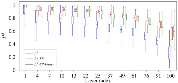
The L 2 parameter regularization, also known as weight decay, is com- monly used in machine learning and especially when training deep neural networks.. This simple

Our models are learned using the transfer learning trick by exploiting deep ar- chitectures that have been pre-trained on imageNet database, and therefore it requires very

performance (10-layer residual-learning networks with the same filter numbers n = 64 and filter size f = 3 over 20 training epochs using Adam optimization and tested with

Deep Learning for Metagenomic Data: using 2D Embeddings and Convolutional Neural Networks.. Nguyen Thanh Hai, Yann Chevaleyre, Edi Prifti, Nataliya Sokolovska,

Efficient natural image segmentation can be achieved thanks to deep fully convolutional network (FCN) and transfer learning [1]. In this paper, we propose to rely on this same method

Bilmes, “Acoustic classification using semi-supervised deep neural networks and stochastic entropy- regularization over nearest-neighbor graphs,” in IEEE Interna- tional Conference