HAL Id: hal-01635455
https://hal.archives-ouvertes.fr/hal-01635455v2
Submitted on 17 Aug 2019
HAL is a multi-disciplinary open access
archive for the deposit and dissemination of sci-entific research documents, whether they are pub-lished or not. The documents may come from teaching and research institutions in France or
L’archive ouverte pluridisciplinaire HAL, est destinée au dépôt et à la diffusion de documents scientifiques de niveau recherche, publiés ou non, émanant des établissements d’enseignement et de recherche français ou étrangers, des laboratoires
Multiscale brain MRI super-resolution using deep 3D
convolutional networks
Chi-Hieu Pham, Carlos Tor-Díez, Hélène Meunier, Nathalie Bednarek, Ronan
Fablet, Nicolas Passat, François Rousseau
To cite this version:
Chi-Hieu Pham, Carlos Tor-Díez, Hélène Meunier, Nathalie Bednarek, Ronan Fablet, et al.. Multiscale brain MRI super-resolution using deep 3D convolutional networks. Computerized Medical Imaging and Graphics, Elsevier, 2019, 77, pp.101647. �10.1016/j.compmedimag.2019.101647�. �hal-01635455v2�
Multiscale brain MRI super-resolution using deep 3D convolutional
1networks
2Chi-Hieu Phama,∗, Carlos Tor-D´ıeza, H´el`ene Meunierb, Nathalie Bednarekb,d, Ronan 3
Fabletc, Nicolas Passatd, Fran¸cois Rousseaua 4
aIMT Atlantique, LaTIM U1101 INSERM, UBL, Brest, France
5
bService de m´edecine n´eonatale et r´eanimation p´ediatrique, CHU de Reims, France
6
cIMT Atlantique, LabSTICC UMR CNRS 6285, UBL, Brest, France
7
dUniversit´e de Reims Champagne-Ardenne, CReSTIC, Reims, France
8
Abstract 9
The purpose of super-resolution approaches is to overcome the hardware limitations 10
and the clinical requirements of imaging procedures by reconstructing high-resolution im-11
ages from low-resolution acquisitions using post-processing methods. Super-resolution tech-12
niques could have strong impacts on structural magnetic resonance imaging when focusing 13
on cortical surface or fine-scale structure analysis for instance. In this paper, we study deep 14
three-dimensional convolutional neural networks for the super-resolution of brain magnetic 15
resonance imaging data. First, our work delves into the relevance of several factors in the 16
performance of the purely convolutional neural network-based techniques for the monomodal 17
super-resolution: optimization methods, weight initialization, network depth, residual learn-18
ing, filter size in convolution layers, number of the filters, training patch size and number 19
of training subjects. Second, our study also highlights that one single network can effi-20
ciently handle multiple arbitrary scaling factors based on a multiscale training approach. 21
Third, we further extend our super-resolution networks to the multimodal super-resolution 22
using intermodality priors. Fourth, we investigate the impact of transfer learning skills onto 23
super-resolution performance in terms of generalization among different datasets. Lastly, 24
the learnt models are used to enhance real clinical low-resolution images. Results tend to 25
demonstrate the potential of deep neural networks with respect to practical medical image 26
applications. 27
Keywords: super-resolution, 3D convolutional neural network, brain MRI
28
∗Corresponding author
Email addresses: [email protected] (Chi-Hieu Pham),
[email protected] (Carlos Tor-D´ıez), [email protected] (H´el`ene Meunier), [email protected] (Nathalie Bednarek), [email protected] (Ronan Fablet), [email protected] (Nicolas Passat), [email protected] (Fran¸cois Rousseau)
1. Introduction 29
Magnetic Resonance Imaging (MRI) is a powerful imaging modality for in vivo brain 30
visualization with a typical image resolution of 1mm. Acquisition time of MRI data and 31
signal-to-noise ratio are two parameters that drive the choice of an appropriate image reso-32
lution for a given study. The accuracy of further analysis such as brain morphometry can be 33
highly dependent on image resolution. Super-Resolution (SR) aims to enhance the resolution 34
of an imaging system using single or multiple data acquisitions (Milanfar 2010). Increas-35
ing image resolution through super-resolution is a key to more accurate understanding of 36
the anatomy (Greenspan 2008). Previous works have shown that applying super-resolution
37
techniques leads to more accurate segmentation maps of brain MRI data (Rueda et al. 2013; 38
Tor-D´ıez et al. 2019) or cardiac data (Oktay et al. 2016). 39
The use of SR techniques has been studied in many works in the context of brain MRI 40
analysis: structural MRI (Manj´on et al. 2010b;Rousseau et al. 2010a; Manj´on et al. 2010a; 41
Rueda et al. 2013;Shi et al. 2015), diffusion MRI (Scherrer et al. 2012;Poot et al. 2013;
Fogt-42
mann et al. 2014; Steenkiste et al. 2016), spectroscopy MRI (Jain et al. 2017), quantitative 43
T1 mapping (Ramos-Llord´en et al. 2017; Van Steenkiste et al. 2017), fusion of orthogonal 44
scans of moving subjects (Gholipour et al. 2010; Rousseau et al. 2010b; Kainz et al. 2015; 45
Jia et al. 2017). The development of efficient and accurate SR techniques for 3D MRI data 46
could be a major step forward for brain studies. 47
Most SR methods rely on the minimization of a cost function consisting of a fidelity term 48
related to an image acquisition model and a regularization term that constrains the space 49
of solutions. The observation model is usually a linear model including blurring, motion, 50
the effect of the point spread function (PSF) and downsampling. The regularizer, which 51
guides the optimization process while avoiding unwanted image solutions, can be defined 52
using pixel-based `2-norm term (Gholipour et al. 2010), total variation (Shi et al. 2015), 53
local patch-based similarities (Manj´on et al. 2010b,a;Rousseau et al. 2010a), sparse coding 54
(Rueda et al. 2013), low rank property (Shi et al. 2015). 55
In particular, the choice of this regularization term remains difficult as it modifies implic-56
itly the space of acceptable solutions without any guaranty on the reconstruction of realistic 57
high-resolution images. Conversely, in a supervised context (in which one can exploit a 58
learning database with low-resolution (LR) and high-resolution (HR) images), the SR of 59
MRI data can be fully driven by examples. The key challenge of supervised techniques is 60
then to accurately estimate the mapping operator from the LR image space to the HR one. 61
Recently, significant advances were reported in SR for computer vision using convolutional 62
neural networks (CNN). This trend follows the tremendous outcome of CNN-based schemes 63
for a wide range of computer vision applications, including for instance image classifica-64
tion (Krizhevsky et al. 2012; Simonyan and Zisserman 2014;He et al. 2016), medical image 65
segmentation (Kamnitsas et al. 2017) or medical image analysis (Tajbakhsh et al. 2016). 66
CNN architectures have become the state-of-the-art for image SR. Initially, Dong et al.
67
(2016a) proposed a three-layer CNN architecture. The first convolutional layer implicitly 68
extracts a set of feature maps for the input LR image; the second layer maps these feature 69
maps nonlinearly to HR patch representations; and the third layer reconstruct the HR 70
image from these patch representations. Several studies have further investigated CNN-71
based architectures for image SR. Among others, the following features have been reported 72
to improve SR performance: an increased depth of the network (Kim et al. 2016a), residual 73
block (with batch normalization and skip connection) (Ledig et al. 2017), sub-pixel layer (Shi
74
et al. 2016), perceptual loss function (instead of mean squared error-based cost functions) 75
(Johnson et al. 2016; Ledig et al. 2017; Zhao et al. 2017), recurrent networks (Kim et al.
76
2016b), generative adversarial networks (Ledig et al. 2017;Pham et al. 2019). Very recently, 77
Chen et al.(2018) proposed a 3D version of densely connected networks (Huang et al. 2017) 78
for brain MRI SR. Inspired by the work byJog et al. (2016),Zhao et al.(2018) investigated 79
self super-resolution for MRI using enhanced deep residual networks (Lim et al. 2017). 80
Recently, very deep architectures obtained the best performance in a challenge focusing 81
on natural image SR (NTIRE 2017 challenge, Timofte et al. 2017). However, due to the
82
variety of the proposed methods and the high number of parameters for the networks ar-83
chitecture design, it is currently difficult to identify the key elements of a CNN architecture 84
to achieve good performance for image SR and assess their applicability in the context of 85
3D brain MRI. In addition the extension of CNN architectures to 3D images, taking into 86
account floating and possibly anisotropic scaling factors may be of interest to address the 87
wide range of possible clinical acquisition settings, whereas classical CNN architectures only 88
address a predefined (integer) scaling factor. The availability of multimodal imaging setting 89
also questions the ability of CNN architectures to benefit from such multimodal data to 90
improve the SR of a given modality. 91
Contributions: This work presents a comprehensive review of deep convolutional neural 92
networks, and associated key elements, for brain MRI SR. Following Timofte et al. (2016), 93
who have experimentally shown several ways to improve SR techniques from a baseline ar-94
chitecture, we study the impact of eight key elements on the performance of convolutional 95
neural networks for 3D brain MRI SR. We demonstrate empirically that residual learning 96
associated with appropriate optimization methods can significantly reduce the time of the 97
training step and fast convergence can be achieved in 3D SR context. Overall, we report 98
better performance when learning deeper fully 3D convolution neural networks and using 99
larger filters. Interestingly, we demonstrate that a single network can handle multiple arbi-100
trary scale factors efficiently, for example, from 2 × 2 × 2mm to 2 × 2 × 1mm or 1 × 1 × 1mm, 101
by learning multiscale residuals from spline-interpolated image. We also report significant 102
improvement using a multimodal architecture, where a HR reference image can guide the 103
CNN-based SR of a given MRI volume. Moreover, we demonstrate that our model can trans-104
fer the rich information available from high-resolution experimental dataset to lower-quality 105
clinical image data. 106
2. Super-Resolution using Deep Convolutional Neural Networks 107
2.1. Learning-based SR 108
Single image SR is a typically ill-posed inverse problem that can be stated according to 109
the following linear formulation: 110
where Y ∈ Rnand X ∈ Rmdenote a LR image and a HR image, H ∈ Rm×nis the observation 111
matrix (m > n) and N denotes an additive noise. D↓ represents the downsampling operator 112
and B is the blur matrix. The purpose of SR methods is to estimate X from the observations 113
Y. The SR image can be estimated by minimizing a least-square cost function: 114
b
X = arg min
X kY − HXk
2. (2)
The minimization of the Equation (2) usually leads to unstable solutions and requires the use 115
of appropriate regularization terms on X. Adding prior knowledge on the image solution 116
(such as piecewise smooth image) may lead to unrealistic solution. In a learning-based 117
context where a set of image pairs (Xi, Yi) is available, the objective is to learn the mapping 118
from the LR images Yi to the HR images Xi, leading to the following formulation: 119 b X = arg min X kX − H −1 Yk2. (3)
In this setting, the matrix H−1 can be modeled as a combination of a restoration matrix
120
F ∈ Rm×m and an upscaling interpolation operator S↑
: Rn → Rm. Given a set of HR
121
images Xi and their corresponding LR images Yi with K samples, the restoration operator
122
F can be estimated as follows: 123 b F = arg min F K X i=1 kXi− F (S↑Yi)k2 = arg min F K X i=1 kXi− F (Zi)k2 (4)
where Z ∈ Rm is the interpolated LR (ILR) version of Y (i.e. Z = S↑Y). F is then a
124
mapping from the ILR image space to the HR image space. 125
SR is the process of estimating HR data from LR data. The main goal is then to estimate 126
high-frequency components from LR observations. Instead of learning the mapping directly 127
from the LR space to the HR one, it might be easier to estimate a mapping from the LR 128
space to the missing high-frequency components, also called the residual between HR and 129
LR data: R = X − Z or equivalently X = Z + R. This approach can be modeled by a skip 130
connection in the network. In such a residual-based modeling, one typically assumes that R 131
is a function of Z. The computation of HR data is then expressed as follows: X = Z + F (Z) 132
where F can be learnt using the following equation: 133 b F = arg min F K X i=1 k(Xi− Zi) − F (Zi)k2. (5)
2.2. CNN-based baseline architecture 134
In this paper, we focus on the learning of the mapping F with convolutional neural 135
networks. Following Dong et al. (2016a) and Kim et al. (2016a), the mapping F from Z
136
to (X − Z) is decomposed into nonlinear operations that correspond to the combination of 137
convolution-based and rectified linear unit (ReLU) layers. 138
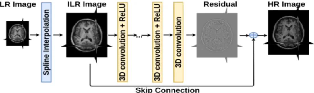
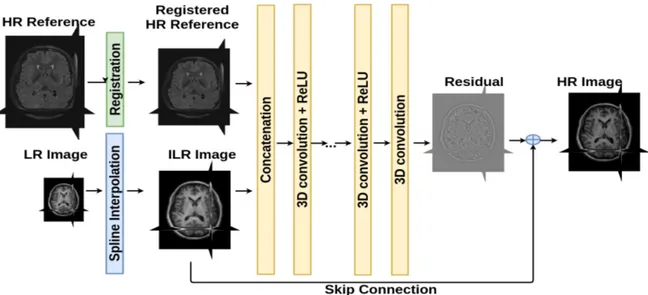
The baseline architecture used in this work can be described as follows: 139
Figure 1: 3D deep neural network for single brain MRI super-resolution.
F1(Z) = max(0, W1∗ Z + B1)
Fi(Z) = max(0, Wi∗ Fi−1(Z) + Bi) for 1 < i < L
FL(Z) = WL∗ FL−1(Z) + BL
(6) where:
140
• L is the number of layers, 141
• Wi and Bi are the parameters of convolution layers to learn. Wi corresponds to ni 142
convolution filters of support c × fi× fi× fi, where c is the number of channels in the 143
input of layer i, fi and ni are respectively the spatial size of the filters and the number 144
of filters of layer i, 145
• max(0, ·) refers to a ReLU applied to the filter responses. 146
This network architecture is depicted in Figure1. Please note that, for instance, the SRCNN 147
model proposed by Dong et al. 2016a corresponds to a specific parameterization of this
148
baseline architecture with f1 = 9, f2 = 1, f3 = 5, n1 = 64, n2 = 32 and no skip connection. 149
The performance of a given architecture depends on several parameters such as the filter 150
size fi, the number of filters ni, the number of layers L, etc. Understanding how these 151
parameters influence the reconstruction of the HR image with respect to the considered 152
application setting (e.g., number of training samples, image size, scaling factor) is a key issue, 153
which remains poorly explored. For instance, regarding the number of layers, it is commonly 154
believed that the deeper the better (Simonyan and Zisserman 2014; Kim et al. 2016a).
155
However, adding layers increases the number of parameters and can lead to overfitting. In 156
particular, previous works (Dong et al. 2016a;Oktay et al. 2016), have shown that a deeper 157
structure does not always lead to better results (Dong et al. 2016a). 158
Specifically focusing on MRI data, the specific objectives of this study are: i) the eval-159
uation and understanding of the effect of key elements of CNN for brain MRI SR, ii) the 160
experimental study of arbitrary multiscale SR using CNN, iii) investigating multimodality-161
guided SR using CNN. 162
3. Sensitivity Analysis of the Considered Architecture 163
In this section, we present the MRI datasets used for evaluation and the key elements of 164
CNN architecture to achieve good performance for single image SR. 165
3.1. MRI Datasets and LR simulation 166
To evaluate SR performances of CNN-based architectures, we have used two MRI datasets: 167
the Kirby 21 dataset and the NAMIC Brain Multimodality dataset. 168
The Kirby 21 dataset (Landman et al. 2011) consists of MRI scans of twenty-one healthy 169
volunteers with no history of neurological conditions. Magnetization prepared gradient echo 170
(MPRAGE, T1-weighted) scans were acquired using a 3T MR scanner (Achieva, Philips 171
Healthcare, The Netherlands) with a 1.0 × 1.0 × 1.2mm3 resolution over an FOV of 240 ×
172
204×256mm acquired in the sagittal plane. Flair data were acquired using 1.1×1.1×1.1mm3
173
resolution over an FOV of 242×180×200mm acquired in the sagittal plane. The T2-weighted 174
volumes were acquired using a 3D multi-shot turbo-spin echo (TSE) with a TSE factor of 175
100 with over an FOV of 200 × 242 × 180mm including a sagittal slice thickness of 1mm. 176
MR images of NAMIC Brain Multimodality1 dataset have been acquired using a 3T
177
GE at BWH in Boston, MA. An 8 Channel coil was used in order to perform parallel 178
imaging using ASSET (Array Spatial Sensitivity Encoding techniques, GE) with a SENSE-179
factor (speed-up) of 2. The structural MRI acquisition protocol included two MRI pulse 180
sequences. The first results in contiguous spoiled gradient-recalled acquisition (fastSPGR) 181
with the following parameters: TR=7.4ms, TE=3ms, TI=600, 10 degree flip angle, 25.6cm2
182
field of view, matrix=256 × 256. The voxel dimensions are 1 × 1 × 1mm3. The second XETA
183
(eXtended Echo Train Acquisition) produces a series of contiguous T2-weighted images 184
(TR=2500ms, TE=80ms, 25.6cm2 field of view, 1 mm slice thickness). Voxel dimensions
185
are 1 × 1 × 1mm3. 186
As in Shi et al. 2015 and Rueda et al. 2013, LR images have been generated from a
187
Gaussian blur and a down-sampling by isotropic scaling factors. In the training phase, a 188
set of patches of training images is randomly extracted. In the baseline setting, the training 189
dataset comprises 10 subjects (3 200 patches 25 × 25 × 25 per subject randomly sampled) 190
and the testing dataset is composed of 5 subjects. During the testing step, the network 191
is applied on the whole images. The peak signal-to-noise ratio (PSNR) in decibels (dB) is 192
used to evaluate the SR results with respect to the original HR images. No denoising or 193
bias correction algorithms were applied to the data. Image intensity has been normalized 194
between 0 and 1. The following figures are drawn based on the average PSNR over all test 195
images. 196
3.2. Baseline and benchmarked architectures 197
The network architecture that is used as a baseline approach in this study is illustrated 198
in Figure 1. The baseline network is a 10 blocks (convolution+ReLU) network with the
199
following parameters: 64 convolution filters of size (3 × 3 × 3) at each layer, mean squared 200
error (MSE) as loss function, weight initialization by He et al.(2015) (MSRA filler), Adam 201
(adaptive moment estimation) method for optimization (Kingma and Ba 2015), 20 epochs
202
on Nvidia GPU and using Caffe package (Jia et al. 2014), batch size of 64, learning rate 203
set to 0.0001, no regularization or drop out has been used. The learning rate multipliers 204
of weights and biases are 1 and 0.1, respectively. For benchmarking purposes, we consider 205
two other state-of-the-art SR models: low-rank total variation (LRTV) (Shi et al. 2015) and 206
SRCNN3D (Pham et al. 2017). SRCNN3D (Pham et al. 2017), which is a 3D extension of
207
the method described in (Dong et al. 2016a), has 3 convolutional layers with the size of 93, 208
13 and 53, respectively. The layers of SRCNN3D consist of 64 filters, 32 filters and one filter, 209
respectively. 210
The next sections present the impact of the key parameters studied in this work: op-211
timization method, weight initialization, residual-based model, network depth, filter size, 212
filter number, training patch size and size of training dataset. 213 3.3. Optimization Method 214 0 10 20 30 40 50 60
Epochs
32 33 34 35 36 37 38 39PS
N
R
(d
B
)
Spline Interpolation LRTV SRCNN3D+ SGD
SRCNN3D + Adam
10L-ReCNN + NAG
10L-ReCNN + SGD-GC
10L-ReCNN + RMSProp
10L-ReCNN + Adam
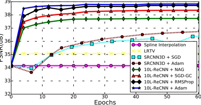
Figure 2: Impact of the optimization methods onto SR performance: SGD-GC, NAG, RMSProp and Adam optimisation of a 10L-ReCNN (10-layer residual-learning network with f = 3 and n = 64). We used Kirby 21 for training and testing with isotropic scaling factor ×2. The initial learning rates of SGD-GC, NAG, RMSProp and Adam are set respectively to 0.1, 0.0001, 0.0001 and 0.0001. These learning rates are decreased by a factor of 10 every 20 epochs. The momentum of these methods, except RMSProp, is set to 0.9. All optimization methods use the same weight initialization described byHe et al.(2015).
Given a training dataset which consists of pairs of LR and HR images, network parame-215
ters are estimated by minimizing the objective function using optimization algorithms. These 216
algorithms play a very important role in training neural networks. The more efficient and 217
effective optimization strategies lead to faster convergence and better performance. More 218
precisely, during the training step, the estimation of the restoration operator F corresponds 219
to the minimization of the objective function L in Equation (5) over network parameters
220
θ = {Wi, Bi}i=1,...,L. 221
Most optimization methods for CNNs are based on gradient descent. A classical method 222
applies a mini-batch stochastic gradient descent with momentum (SGD) (LeCun et al. 1998) 223
as used by Dong et al. (2016a); Pham et al. (2017). However, the use of fixed momentum 224
causes numerical instabilities around the minimum. Nesterov’s accelerated gradient (NAG) 225
(Nesterov 1983) was proposed to cope with this issue but the use of small learning rates 226
induces slow convergence. By contrast, high learning rates may lead to exploding gradients 227
(Bengio et al. 1994; Glorot and Bengio 2010). In order to address this issue, Kim et al.
228
(2016a) proposed the stochastic gradient descent method with an adjustable gradient clip-229
ping (SGD-GC) (Pascanu et al. 2013) to achieve an optimization with high learning rates. 230
The predefined range over which gradient clipping is applied may still cause SGD-GC not 231
to converge quickly or make difficult the tuning of a global learning rate. Recently, methods 232
have been proposed to address this issue through an automatic adaption of the learning rate 233
for each parameter to be learnt. RMSProp (root-mean-square propagation) (Tieleman and
234
Hinton 2012) and Adam (adaptive moment estimation) (Kingma and Ba 2015) are the two 235
most popular models in this category. 236
The results of four optimization methods (NAG, SGD-GC, RMSProp and Adam) for 237
the baseline network are illustrated in Figure 2. Firstly, regardless the method used, the 238
baseline network shows better performance than LRTV (Shi et al. 2015) and SRCNN3D
239
(Pham et al. 2017). Secondly, it can be observed that the baseline network can converge very 240
rapidly (only 20 epochs with small learning rate of 0.0001). Finally, in these experiments, 241
the most efficient and effective optimization method is Adam as regards both PSNR metric 242
and convergence speed. Hence, in the next sections, we use Adam method with β1 = 0.9
243
and β2 = 0.999 to train our networks with 20 epochs. 244
3.4. Weight Initialization 245
The optimization algorithms for training a CNN are typically initialized randomly. In-246
appropriate initialization can lead to long time convergence or even divergence. Several 247
studies (Dong et al. 2016a; Oktay et al. 2016; Pham et al. 2017) used a normal distribu-248
tion N (0, 0.001) to initialize the weights of convolutional filters. However, because of too 249
small initial weights, the optimizer may be stuck into a local minimum especially when 250
building deeper networks. BothDong et al. (2016a) concluded that deeper networks do not 251
lead to better performance, and Oktay et al. (2016) confirmed that the addition of extra 252
convolutional layers to the 7-layer model is found to be ineffective. Uniform distribution 253
U (−p3/(nf3),p3/(nf3)) (called Xavier filler) (Glorot and Bengio 2010) was also proposed 254
to initialize the weights of deeper networks. In order to add more layers to networks, He
255
et al. (2015) suggested an initial training stage by sampling from the normal distribution 256
N (0,p2/(nf3)) (called here Microsoft Research Asia - MSRA filler). 257
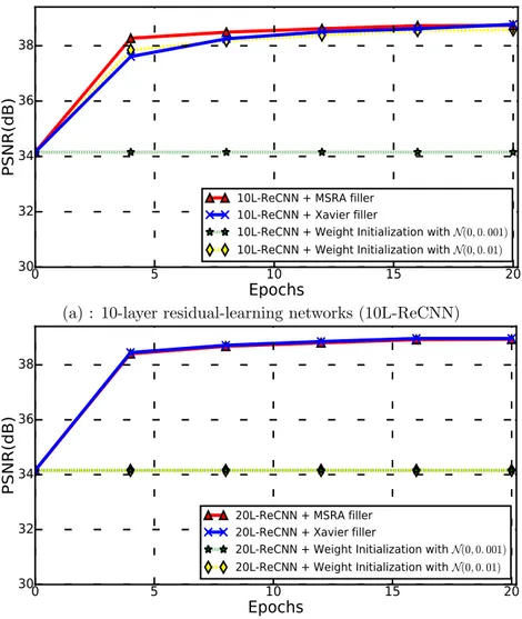
Overall, we evaluate here the weight initialization schemes described byGlorot and
Ben-258
gio(2010) andHe et al.(2015), a normal distribution N (0, 0.001) as proposed byDong et al.
0 5 10 15 20 Epochs 30 32 34 36 38 PS N R (d B )
10L-ReCNN + MSRA filler 10L-ReCNN + Xavier filler
10L-ReCNN + Weight Initialization with N(0, 0. 001) 10L-ReCNN + Weight Initialization with N(0, 0. 01)
(a) : 10-layer residual-learning networks (10L-ReCNN)
0 5 10 15 20 Epochs 30 32 34 36 38 PS N R (d B )
20L-ReCNN + MSRA filler 20L-ReCNN + Xavier filler
20L-ReCNN + Weight Initialization with N(0, 0. 001) 20L-ReCNN + Weight Initialization with N(0, 0. 01)
(b) : 20-layer residual-learning networks (20L-ReCNN)
Figure 3: Weight initialization scheme vs. performance (residual-learning networks with the same filter numbers n = 64 and filter size f = 3 using Adam optimization and tested with isotropic scaling factor ×2 using Kirby 21 for training and testing, 32 000 patches with size 253for training).
(2016a); Oktay et al.(2016) and a normal distribution N (0, 0.01) for the considered SR ar-260
chitecture. Experiments with a deeper architecture were also performed, more precisely for 261
a 20-layer architecture, which is the deepest architecture that could be implemented for 262
the considered experimental setup due to GPU memory setting. As shown in Figure 3,
263
the initialization with normal distributions N (0, 0.001) failed to make the training of both 264
10-layer and 20-layer residual-learning networks converge. In addition, our 20-layer network 265
also does not converge when initialized with normal distributions N (0, 0.01). By contrast, 266
MSRA and Xavier filler schemes make the networks converge and reach similar reconstruc-267
tion performance. For the rest of this paper, we use MSRA weight filler as initialization 268
scheme. 269
3.5. Residual Learning 270
The CNN methods proposed by Dong et al. (2016a); Shi et al. (2016); Dong et al.
271
(2016b) use the LR image as input and outputs the HR one. We refer to such approach 272
as a non-residual learning. Within these approaches, low-frequency features are propagated 273
through the layers of networks, which may increase the representation of redundant features 274
in each layer and in turn the computational efficiency of the training stage. By contrast, 275
one may consider residual learning or normalized HR patch prediction as pointed out by 276
several learning-based SR methods (Zeyde et al. 2012; Timofte et al. 2013,2014; Kim et al.
277
2016a). When considering CNN methods, one may design a network which predicts the 278
residual between the HR image and the output of the first transposed convolutional layer 279
(Oktay et al. 2016). Using residual blocks, a CNN architecture may implicitly embed residual 280
learning while still predicting the HR image (Ledig et al. 2017). 281 0 5 10 15 20 Epochs 34 35 36 37 38 39 PS N R( dB ) Spline Interpolation 10L-ReCNN (Residual) 10L-CNN (Non-residual) 20L-ReCNN (Residual) 20L-CNN (Non-residual)
Figure 4: Non-residual-learning vs Residual-learning networks with the same n = 64 and f3 = 33 and the depths of 10 and 20 (called here 10L-CNN vs 10L-ReCNN and 20L-CNN vs 20L-ReCNN) over 20 training epochs using Adam optimization with the same training strategy and tested with isotropic scale factor ×2 using Kirby 21 for training and testing.
Here, we perform a comparative evaluation of non-residual learning vs. residual learning 282
strategies. Figure4depicts PSNR values and convergence speed of residual vs. non-residual 283
network structures with 10 and 20 convolutional layers. The residual-learning networks 284
converge faster than the non-residual-learning ones. In addition, residual learning leads 285
to improvements in PSNR (+0.4dB for 10 layers and +1.2dB for 20 layers). It might be 286
noted that these experiments do not support the common statement that the deeper, the 287
better for CNNs. Here, the use of additional layers is only beneficial when using residual 288
modeling. Deeper architectures may even lower the reconstruction performance with non-289
residual learning. 290
3.6. Depth, Filter Size and Number of Filters 291
As shown by the previous experiment, the link between network depth and performance 292
remains unclear. Besides, it is hard to train deeper networks because gradient computation 293
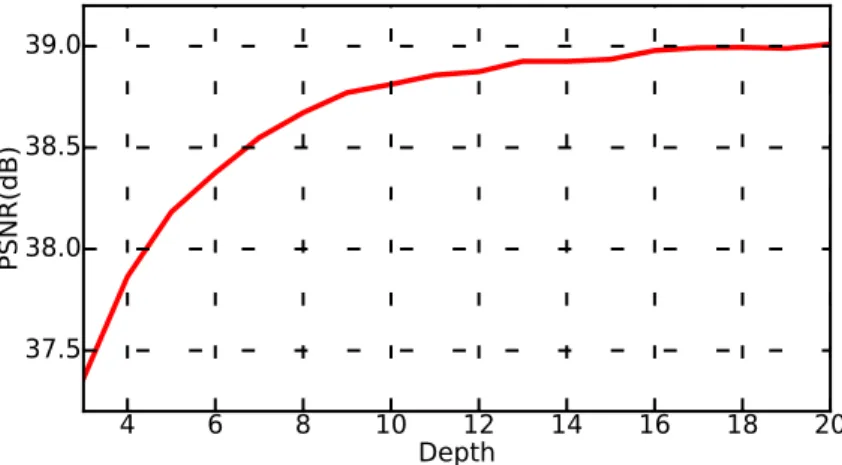
4 6 8 10 12 14 16 18 20 Depth 37.5 38.0 38.5 39.0 PS N R (d B )
Figure 5: Depth vs Performance (residual-learning networks with the same filter numbers n = 64 and filter size f = 3 over 20 training epochs using Adam optimization and tested with isotropic scale factor ×2 using Kirby 21 for training and testing, 32 000 patches with size 253 for training).
can be unstable when adding layers (Glorot and Bengio 2010). For instance, Oktay et al.
294
(2016) tested extra convolutional layers to a 7-layer model but achieved negligible perfor-295
mance improvement. As mentioned in Section 2.2, SRCNN (Dong et al. 2016a) was also
296
tested with deeper architectures but no improvement was reported. However, Kim et al.
297
(2016a) argue that the performance of CNNs for SR could be improved by increasing the 298
depth of network compared to neural network architectures proposed byDong et al.(2016a); 299
Oktay et al. (2016). 300
The previous section supports that deeper architectures may be beneficial when consid-301
ering a residual learning. We now evaluate the reconstruction performance as a function of 302
the number of layers. Results are reported in Figure5. They stress that increasing network 303
depth with residual learning improves the quality of the estimated HR image (e.g. +1.6dB 304
increasing of the depth from 3 to 20 or +0.5dB increasing of the depth from 7 to 20). 305
The parameterization of the convolutional filters is also of key interest. Inspired by the 306
VGG network designed for classification (Simonyan and Zisserman 2014), previous CNN
307
methods for SR mostly focused on small convolutional filters of size (3 × 3 × 3) as proposed 308
by Kim et al. (2016a); Oktay et al. (2016); Kamnitsas et al. (2017). Oktay et al. (2016) 309
even argued that such architecture can lead to better non-linear estimations. Regarding 310
the number of filters for each layer, Dong et al. (2016a) reported greater reconstruction 311
performance when increasing the number of filters. But these experiences were not reported 312
in other CNN-based SR studies (Kim et al. 2016a;Oktay et al. 2016). Here, we both evaluate 313
the effect of the filter size and of the number of filters. 314
Figure 6 shows that a 10-layer network with a filter size of 53 shows results as well as 315
a 20-layer network with 33 filters. Besides reconstruction performance, the use of a larger 316
filter size decreases the training speed and significantly increases the complexity and memory 317
cost for training. For example, it took us 50 hours to train a 10-layer network with a filter 318
size of 53. By contrast, a deeper network with smaller filters (i.e. 20-layer network with 33 319
filters) involves a smaller number of parameters, such that it took us only 24 hours to train. 320
1 3 5 Filter size f3 34 35 36 37 38 39
PS
NR
(dB
)
Spline Interpolation 10L-ReCNN with n = 64 filters20L-ReCNN with n = 64 filters
1 3 5 Filter size f3 0 10 20 30 40 50
Tra
ini
ng
tim
e (
ho
urs)
10L-ReCNN with 20L-ReCNN with n = 64n = 64 filters filters16 32 64 Filter number n 38.0 38.2 38.4 38.6 38.8 39.0
PS
NR
(dB
)
10L-ReCNN with filter size f3= 33 20L-ReCNN with filter size f3= 33
16 32 64 Filter number n 5 10 15 20 25
Tra
ini
ng
tim
e (
ho
urs)
10L-ReCNN with filter size 20L-ReCNN with filter size ff33= 3= 333Figure 6: Impact of convolution filter parameters (sizes f × f × f = f3 with n filters) on PSNR and computation time. These 10-layers residual-learning networks are trained from scratch using Kirby 21 with Adam optimization over 20 epochs and tested with the testing images of the same dataset for isotropic scale factor ×2.
These experiments suggest that deeper architectures with small filters can replace shallower 321
networks with larger filters both in terms of computational complexity and of reconstruction 322
performance. In addition, the increase in the number of filters within networks can increase 323
the performance. However, we were not able to use 128 filters with the baseline architecture 324
due to the limited amount of memory. This stresses out the need to design memory efficient 325
architectures for 3D image processing using deeper CNNs with more filters. 326
3.7. Training Patch Size and Subject Number 327
In the context of brain MRI SR, the acquisition and collection of large datasets with 328
homogeneous acquisition settings is a critical issue. We now evaluate the extent to which 329
the number of training subjects influences SR reconstruction performance. As the training 330
samples are extracted as patches of brain MRI images, we also evaluate the impact of the 331
training patch size on learning and reconstruction performances. 332
The size of training patches should be greater or equal to the size of the receptive field 333
of the considered network (Simonyan and Zisserman 2014;Kim et al. 2016a), which is given 334
by ((f − 1)D + 1)3 for a D-layer network with filter size f3. Figure 7 confirms that better 335
performances can be achieved using larger training patches (from 113 to 313 with the 10-layer 336
network and from 113 to 293 with the 12-layer network). However, if the patch size is larger 337
than the receptive field (e.g. 213 within the 10-layers network and 253 within the 12-layers 338
network), then the improvement is negligible consuming, in the meantime, considerably 339
more GPU memory and training time. 340
We stressed previously that the selection of the network depth involves a trade-off be-341
tween reconstruction performance and GPU memory requirement and training time increase. 342
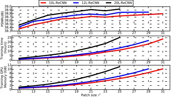
11 13 15 17 19 21 23 25 27 29 31 38.3 38.4 38.5 38.6 38.7 38.8 38.9 39.0 PS N R (d B ) 11 13 15 17 19 21 23 25 27 29 31 0 5 10 15 20 25 Tr a in in g tim e (h ou rs) 11 13 15 17 19 Patch size 21 23 25 27 29 31 τ3 0 2 4 6 8 10 12 Tr ain ing G PU M em or y ( GB )
10L-ReCNN 12L-ReCNN 20L-ReCNN
Figure 7: First row: Training patch size vs. performance. Second row: Patch size vs. training time. Third row: Patch size vs training GPU memory requirement. These networks with the same n = 64 and f3= 33 are trained from scratch using Kirby 21 with batch of 64 and tested with the testing images of the same dataset for isotropic scale factor ×2.
A similar result can be drawn with respect to the patch size. Figure7illustrates that larger 343
training patch sizes also require more memory for training. Moreover, this figure shows that 344
better performance can be achieved using larger training patch sizes. It may be noted that 345
the performance of the 10-layer networks may reach a performance similar to 12-layer and 346
20-layer networks when using larger training patches but it takes more time and more GPU 347
memory for training. 348
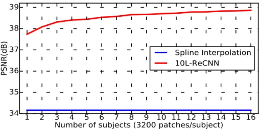
Regarding the number of training subjects, Figure 8 points out that a single subject is 349
enough to reach better performance than spline interpolation. Interestingly, reconstruction 350
performance increases slightly when more subjects are considered, which appears appropriate 351
for real-world applications. However, in fact, more training dataset takes more time within 352
the same experience settings. In the next sections, for saving training time, we propose to 353
use 10 subjects for learning. 354
4. Handling Arbitrary Scales 355
In some CNN-based SR approaches, the networks are learnt for a fixed and specified 356
scaling factor. Thus, a network built for one scaling factor cannot deal with any other 357
scale. In medical imaging, Oktay et al. (2016) have applied CNNs for upscaling cardiac
358
image slices with the scale of 5 (e.g. upscaling the voxel size from 1.25 × 1.25 × 10.0mm to 359
1.25 × 1.25 × 2.00mm). Typically, their network is not capable of handling other scales due 360
to the use of fixed deconvolutional layers. In brain MRI imaging, the variety of the possible 361
acquisition settings motivates us to explore multiscale settings. 362
1 2 3 4 5 6 7 8 9 10 11 12 13 14 15 16
Number of subjects
(3200 patches/subject)34 35 36 37 38 39 PS N R( dB ) Spline Interpolation 10L-ReCNN
Figure 8: Number of subjects vs. performance (10-layer residual-learning networks with the same filter numbers n = 64 and filter size f = 3 over 20 training epochs using Adam optimization and tested with isotropic scale factor ×2 using Kirby 21 for training and testing, 3 200 patches per subject with size 253for training).
Following Kim et al. (2016a), we investigate how we may deal with multiple scales in a 363
single network. It consists of creating a training dataset within which we consider LR and 364
HR image pairs corresponding to different scaling factors. We test two cases: the first case 365
where the learning dataset for combined scale factors (×2, ×3) has the same number as a 366
single scale factor and the second one where we double the learning dataset for multiple 367
scale factors. To avoid a convergence towards a local minimum of one of the scaling factors, 368
we learn network parameters on randomly shuffled dataset. 369
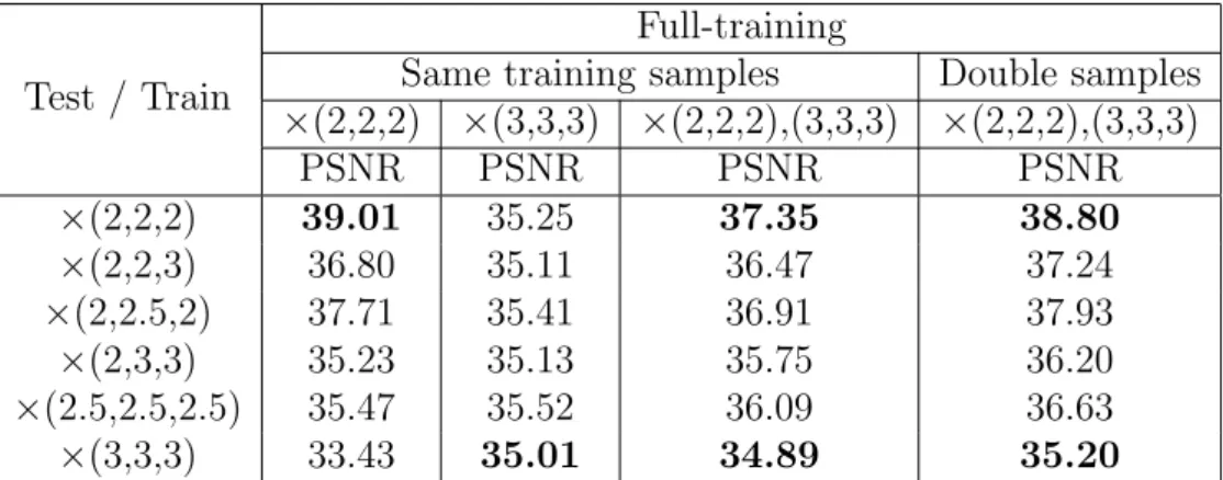
Table 1 summarizes experimental results. First, when the training is achieved for the
370
scaling from (2 × 2 × 2) on a dataset of (2 × 2 × 2) scale, it can be noticed that reconstruction 371
performances decrease significantly when applied to other scaling factors (there is a drop 372
from 39.01dB to 33.43dB when testing with (3 × 3 × 3)). Second, it can be noticed that 373
when the training is performed on multiscale data within the same training samples, there is 374
no significant performance change compared to training from a single-scale dataset. Third, 375
a training dataset with double samples leads to a better performance. Moreover, training 376
from multiple scaling factors leads to the estimation of a more versatile network. Overall, 377
these results show that one single network can handle multiple arbitrary scaling factors. 378
5. Multimodality-guided SR 379
In clinical cases, it is frequent to acquire one isotropic HR image and LR images with 380
different contrasts in order to reduce the acquisition time. Hence, a coplanar isotropic HR 381
image might be considered as a complementary source of information to reconstruct HR 382
MRI images from LR ones (Rousseau et al. 2010a). To address this multimodality-guided
383
SR problem, we add a concatenation layer as the first layer of the network, as illustrated in 384
Figure 9. This layer concatenates the ILR image and a registered HR reference along the
Test / Train
Full-training
Same training samples Double samples
×(2,2,2) ×(3,3,3) ×(2,2,2),(3,3,3) ×(2,2,2),(3,3,3) PSNR PSNR PSNR PSNR ×(2,2,2) 39.01 35.25 37.35 38.80 ×(2,2,3) 36.80 35.11 36.47 37.24 ×(2,2.5,2) 37.71 35.41 36.91 37.93 ×(2,3,3) 35.23 35.13 35.75 36.20 ×(2.5,2.5,2.5) 35.47 35.52 36.09 36.63 ×(3,3,3) 33.43 35.01 34.89 35.20
Table 1: Experiments with multiple isotropic scaling factors with the 20-layers network using the training and testing images of Kirby 21. Bold numbers indicate that the tested scaling factor is present in the training dataset. We test two conditions of same training data and double training data.
channel axis. The registration step of HR reference ensures that the two input images share 386
the same geometrical space. 387
We experimentally evaluate the relevance of the proposed multimodality-guided SR 388
model according to the following setting. We investigate whether the complementary use of 389
a Flair or a T2-weighted MRI image might be beneficial to improve the resolution of a LR 390
T1-weighted MRI image. Concerning the Kirby 21 dataset, we apply an affine transform 391
estimated using FSL (Jenkinson et al. 2012) to register images of a same subject into a com-392
mon coordinate space. We assume here that the affine registration can compensate motion 393
between two scans during the same acquisition session. This appears a fair assumption since 394
here we are considering an organ that does not undergo significant deformation between two 395
acquisitions. The registration step has been checked visually for all the images. Data of the 396
NAMIC dataset are already in the same coordinate space so no registration step is required. 397
Figure10shows the results of the multimodality-guided SR compared to the monomodal
398
SR for both Kirby dataset (a) and NAMIC datasets (b). It can be seen that multimodal-399
ity driven approach can lead to improved reconstruction results. In these experiments, the 400
overall upsampling result depends on the quality of the HR image used to drive the re-401
construction process. Thus, adding high resolution information containing artifacts limits 402
reconstruction performance. This is especially the case for the Kirby dataset. For instance, 403
when considering T2w images, no improvement is observed for Kirby dataset and an im-404
provement greater than 1dB is reported for NAMIC dataset. As the T2w image resolution 405
is lower than T1w modality in Kirby dataset, these results may emphasize the requirement 406
for actual HR information to expect significant gain w.r.t. the monomodal model. Figure 407
11shows visually that edges in the residual image between the ground truth and the recon-408
struction by the multimodal approach are reduced significantly compared to interpolation 409
and monomodal methods (e.g. the regions of lateral ventricles). This means that the mul-410
timodal approach resulting the reconstructions which are the most similar to the ground 411
truth. These qualitative results highlight the fact that the proposed multimodal method 412
provides a better performance than other compared methods. 413
Figure 9: 3D deep neural network for multimodal brain MRI super-resolution using intermodality priors. Skip connection computes the residual between ILR image and HR image.
In addition, we explore the impact of the network depth augmentation with regard to 414
the performance of multimodal SR approach. The experiments shown in Figure 12indicate
415
that the deeper structures do not lead to better results within the multimodal method. 416
6. How Transferable are learnt Features? 417
Training a CNN from scratch requires a substantial amount of training data and may 418
take a long time. Moreover, to avoid overfitting, the training dataset has to reflect the 419
appearance variability of the images to reconstruct. In the context of brain MRI, part of 420
image variability comes from acquisition systems. Hence, we investigate the impact of such 421
image variability onto SR performance by evaluating transfer learning skills among different 422
datasets corresponding to the same imaging modality. 423
In order to characterize such generalization skills, we evaluate in which extent the selec-424
tion of a given training dataset influences the reconstruction performance of the network. 425
To this end, we train from scratch two 20L-ReCNN networks separately for a 10-image 426
NAMIC T1-weighted dataset and a 10-image Kirby T1-weighted dataset, and we test the 427
trained models for the remaining 10-image NAMIC and Kirby T1-weighted datasets. The 428
considered case-study involves a scaling factor of (2 × 2 × 2). For quantitative compari-429
son, the PSNR and the structural similarity (SSIM) (the definition of SSIM can be found 430
in Wang et al. 2004) are used to evaluate the performance of each model in Table 2. For 431
benchmarking purposes, we also include a comparison with the following methods: cubic 432
spline interpolation, low-rank total variation (LRTV) (Shi et al. 2015), SRCNN3D (Pham
433
et al. 2017). The use of 20-layer CNN-based approaches for each training dataset can lead 434
to improvements over spline interpolation, LRTV method and SRCNN3D (with respect to 435
both PSNR and SSIM). Although, the gain is slightly lowered (e.g. PSNR: 0.55dB for test-436
ing Kirby and 0.74dB for NAMIC, SSIM: 0.003 for Kirby and 0.0019 for NAMIC) when 437
0 5 10 15 20 Epochs 34 35 36 37 38 39 PS NR
(dB
)
Spline Interpolation10L-ReCNN for LR T1w (Monomodal)
10L-ReCNN for LR T1w + registered HR T2w
10L-ReCNN for LR T1w + registered HR Flair 10L-ReCNN for LR T1w + registered HR Flair and T2w
(a) Multimodal experiments using Kirby 21 dataset for training and testing.
0 5 10 15 20 Epochs 34 35 36 37 38 39 PS NR
(dB
)
Spline Interpolation10L-ReCNN for LR T1w (Monomodal) 10L-ReCNN for LR T1w + HR T2w
(b) Multimodal experiments using NAMIC dataset for training and testing.
Figure 10: Multimodality-guided SR experiments. The LR T1-weighted images are upscaled with isotropic scale factor ×2 using respectively monomodal network (10L-ReCNN for LR T1w), HR T2w multimodal network, HR Flair multimodal network and both HR Flair and T2w multimodal images.
using different training and testing dataset (i.e. different resolution), our proposed networks 438
obtain better results than compared methods. 439
For qualitative comparison, Figures 13 and 14 show the results of reconstructed 3D
440
images obtained from all the compared techniques. The zoom version of the reconstructions 441
20L-ReCNN shows sharpen edges and a grayscale intensity which are closest to the ground 442
truth. In addition, the HR reconstruction of the 20L-ReCNN model shows that its differences 443
from the ground truth are less than other methods (i.e. the contours of the residual image 444
of the 20L-ReCNN method are less visible than those of others). Hence, we can infer that 445
our proposed method better preserves contours, geometrical structures and better recovers 446
the image contrast compared with the other methods. 447
7. Application of Super-Resolution on Clinical Neonatal Data 448
In clinical routine, anisotropic LR MRI data are usually acquired in order to limit the 449
acquisition time due to patient comfort such as infant brain MRI scans (Makropoulos et al., 450
2018), or in case of rapid emergency scans (Walter et al., 2003). These images usually have 451
a high in-plane resolution and a low through-plane resolution. Anisotropic data acquisition 452
(a) Original HR T1-weighted (b) LR T1-weighted image (c) HR T2-weighted reference
(d) Spline Interpolation (e) Monomodal 10L-ReCNN (f) Multimodal 10L-ReCNN
Figure 11: Illustration of the axial slices of monomodal and multimodal SR results (subject 01018, patho-logical case of testing set) with isotropic voxel upsampling using NAMIC. The LR T1-weighted image (b) with voxel size 2 × 2 × 2mm3 is upsampled to size 1 × 1 × 1mm3. The monomodal network 10L-ReCNN is applied directly the LR T1-weighted image (b), whereas the multimodal network 10L-ReCNN uses the HR T2-weighted reference (c) to upscale LR T1-weighted image (b). The results of the monomodal and multimodal networks are shown in (e) and (f), respectively. The different between ground truth image and reconstruction results are at the bottom. Their zoom version are at the right.
severely limits the 3D exploitation of MRI data. Interpolation is commonly used to upsam-453
pled these LR images to isotropic resolution. However, interpolated LR images may lead to 454
partial volume artifacts that may affect segmentation (Ballester et al.,2002). In this section, 455
we aim to use our single image SR method to enhance the resolution of such clinical data. 456
The idea is to apply our proposed convolutional neural networks-based SR method to 457
transfer the rich information available from high-resolution experimental dataset to lower-458
quality image data. The procedure first uses CNNs to learn mappings between real HR 459
images and their corresponding simulated LR images with the same resolution of real data. 460
The LR data is generated by the observation model, which is decomposed into a linear 461
downsampling operator after a space-invariant blurring model as a Gaussian kernel with 462
the full-width-at-half-maximum (FWHM) equal to slice thickness (Greenspan, 2008). Once
463
models are learnt, these mappings enhance the LR resolution of unseen low quality images. 464
In order to verify the applicability of our CNN-based methods, we have used two neona-465
tal brain MRI dataset: the Developing Human Connectome Project (dHCP) (Hughes et al.,
466
2017) and clinical neonatal MRI data acquired in the neonatology service of Reims
Hos-467
pital (Multiphysics image-based AnalysIs for premature brAin development understanding 468
4 6 8 10 12 14 16 18 20 Depth 38.0 38.2 38.4 38.6 38.8 39.0 39.2 PS N R (d B )
Figure 12: Depth vs. performance (multimodal SR using residual-learning networks with the same filter numbers n = 64 and filter size f = 3 over 20 training epochs using Adam optimization and tested with isotropic scale factor ×2 using NAMIC for training and testing).
Testing dataset
Spline Interpolation LRTV SRCNN3D 20L-ReCNN
Kirby (10 images) Kirby (10 images) NAMIC(10 images)
PSNR SSIM PSNR SSIM PSNR SSIM PSNR SSIM PSNR SSIM
Kirby (5 images ) 34.16 0.9402 35.08 0.9585 37.51 0.9735 38.93 0.9797 38.06 0.9767 Standard deviation 1.90 0.0111 2.09 0.0083 1.97 0.0053 1.87 0.0044 1.83 0.0045 Gain - - 0.92 0.0183 3.36 0.0333 4.77 0.0395 3.9 0.0365 NAMIC (10 images) 33.78 0.9388 34.34 0.9549 36.72 0.9694 37.73 0.9762 38.28 0.9781 Standard deviation 1.82 0.0071 1.79 0.0044 1.76 0.0035 1.81 0.0031 1.78 0.0029 Gain - - 0.56 0.0161 2.94 0.0306 3.95 0.0374 4.5 0.0393
Table 2: The results of PSNR/SSIM for isotropic scale factor ×2 with the gain between compared methods and the method of spline interpolation. One network 20L-ReCNN trained with 10 images of Kirby and one trained with NAMIC
- MAIA dataset). The HR images are T2-weighted MRIs of the dHCP and provided by 469
the Evelina Neonatal Imaging Centre, London, UK. Forty neonatal data were acquired on 470
a 3T Achieva scanner with repetition (TR) of 12 000 ms and echo times (TE) of 156ms, 471
respectively. The size of voxels is 0.5 × 0.5 × 0.5 mm3. In-vivo neonatal LR images has a 472
voxel size of about 0.4464 × 0.4464 × 3 mm3. 473
Figure 15 compares the qualitative results of HR reconstructions (spline interpolation, 474
NMU (Manj´on et al.,2010b) and our proposed networks) of a LR image from MAIA dataset. 475
In this experiment, we do not have the ground truth of real LR data for calculating quanti-476
tative metrics. The comparison reveals that the CNNs-based methods recover shaper images 477
and better defined boundaries than spline interpolation. For instance, the cerebrospinal fluid 478
(CSF) of the cerebellum of the proposed method, in Figure 15, is more visible than those
479
obtained with the compared methods. Our proposed technique reconstructs more curved 480
cortex and more accurate ventricles. These results tend to confirm qualitatively the efficacy 481
of our approach. 482
(a) Original HR (b) LR image (c) Spline Interpolation
(d) LRTV (e) SRCNN3D (f) 20L-ReCNN
Figure 13: Illustration of SR results (subject KKI2009-02-MPRAGE, non-pathological case, in testing set of dataset Kirby 21) with isotropic voxel upsampling. LR data (b) with voxel size 2 × 2 × 2.4mm3is upsampled to size 1 × 1 × 1.2mm3. The difference between the ground truth image and the reconstruction results are in the right bottom corners. Both network SRCNN3D and network 20L-ReCNN are trained with the 10 last images of Kirby.
8. Discussion 483
This study investigates CNN-based models for 3D brain MR image SR. Based on a 484
comprehensive experimental evaluation, we would like to draw the following conclusions 485
and recommendations regarding the setup to be considered. We highlight that eight com-486
plementary factors may drive the reconstruction performance of CNN-based models. The 487
combination of 1) appropriate optimization with 2) weight initialization and 3) residual 488
learning is a key to exploit deeper networks with a faster and effective convergence. The 489
choice of an appropriate optimization method can lead to a PSNR improvement of (at least) 490
1dB. In this study, it has appeared that Adam method (Kingma and Ba 2015) provides
491
significantly better reconstruction results than other classical techniques such as SGD, and a 492
faster convergence. Moreover, weights initialization is a very important step. Indeed, some 493
approaches simply do not achieve convergence in the learning phase. This study has also 494
(a) Original HR (b) LR image (c) Spline Interpolation
(d) Low-Rank Total Variation (LRTV)
(e) 20L-ReCNN (trained with Kirby)
(f) 20L-ReCNN (trained with NAMIC)
Figure 14: Illustration of SR results (subject 01011-t1w, pathological case, in testing set of dataset NAMIC) with isotropic voxel upsampling. LR data (b) with voxel size 2×2×2mm3is upsampled to size 1×1×1mm3. The zoom versions of the axial slices are in the right bottom corners.
shown that residual modeling for single image SR is a straightforward technique to improve 495
the reconstruction performances (+0.4dB) without requiring major changes in the network 496
architecture. Appropriate weight initialization methods described byHe et al. (2015);
Glo-497
rot and Bengio (2010) allow us to build deeper residual-learning networks. From our point 498
of view, these three aspects of SR algorithm are the first to require special attention for the 499
implementation of a SR technique based on CNN. 500
Overall, we show that better performance can be achieved by learning 4) a deeper fully 3D 501
convolution neural network, 5) exploring more filters and 6) increasing filter size. In addition, 502
using 7) larger training patch size and 8) augmentation of training subject leads to increase 503
the performance of the networks. The adjustment of these 5 elements provides a similar 504
improvement (about 0.5dB). Although it seems natural to implement the deepest possible 505
network, this parameter is not always the key to obtaining a better estimate of a high-506
resolution image. Our study shows that, depending on the type of input data (monomodal 507
or multimodal), network depth is not necessarily the main parameter leading to better 508
(a) Original LR image (b) Spline interpolation (c) NMU (d) Our proposed method
Figure 15: Illustration of SR results on a clinical data of MAIA dataset with isotropic voxel upsampling. Original data with voxel size of about 0.4464 × 0.4464 × 3 is resampled to size 0.5 × 0.5 × 0.5 mm3. Networks are trained with the dHCP dataset. The first, second, third and last rows presents the sagittal slices, the zoom versions of the sagittal slices, the coronal slices and the zoom versions of the coronal slices, respectively.
image reconstruction. In addition, it is important to take into account the time of the 509
learning phase as well as the maximum memory available in the GPU in order to choose the 510
best architecture of the network. For instance, for the monomodal SR case based on the 511
simulations of Kirby dataset, we suggest using 20-layer networks with 64 small filters with 512
size of 33 regarding 10 training subjects of size 253 to achieve practicable results. 513
In CNN-based approaches, the upscaling operation can be performed by using transposed 514
convolution (so-called fractionally strided convolutional) layers as proposed byOktay et al.
515
(2016);Dong et al.(2016b) or sub-pixel layers (Shi et al. 2016). However, the trained weights 516
of these networks are totally applied for a specified scale factor. This is a limiting aspect of 517
CNN-based SR for MR data since a fixed upscaling factor is not appropriate in this context. 518
In this study, we have presented a multiscale CNN-based SR method for single 3D brain 519
MRI that is capable of learning multiple scales by training multiple isotropic scale factors 520
(a) Nearest-neighbor (b) Spline interpolation
(c) LRTV (d) 20L-ReCNN
Figure 16: Illustration of SR results (subject 01018-t1w in testing set of dataset NAMIC) with isotropic voxel upsampling. Original data with voxel size of 1 × 1 × 1 mm3 is upsampled to size 0.5 × 0.5 × 0.5 mm3. 20L-ReCNN is trained with the NAMIC dataset.
due to an independent upsampling technique such as spline interpolation. Handling multiple 521
scales is related to multi-task learning. The lack of flexibility of learnt network architectures 522
raises an open issue motivating further studies: how can we build a network that can deal 523
with a set of observation models (i.e. multiple scales, arbitrary point spread functions, non 524
uniform sampling, etc.)? For instance, when applying SR techniques in a realistic setting, 525
the choice of the PSF is indeed a key element for SR methods and it depends on the type 526
of MRI sequence. More specifically, the shape of the PSF depends on the trajectory in the 527
k-space (Cartesian, radial, spiral). Making the network independent from the PSF model 528
(i.e. doing blind SR) would be a major step for its use in routine protocol. Further research 529
directions could focus on making more flexible CNN-based SR methods for greater use of 530
these techniques in human brain mapping studies. 531
Evaluation of SR techniques is carried out on simulated LR images. However, one po-532
tential use of SR techniques would be to improve the resolution of isotropic data acquired in 533
clinical routine. Figure 16 shows upsampling results on isotropic T1-weighted MR images
534
(the resolution was increased from 1 × 1 × 1mm3 to 0.5 × 0.5 × 0.5mm3). In this experi-535
ment, the applied network has been trained to increase image resolution from 2 × 2 × 2mm3 536
to 1 × 1 × 1mm3. Although quantitative results cannot be computed, visual inspection
537
of reconstructed upsampled images tend to show the potential of this SR method. Thus, 538
features learnt at a lower scale (2mm in this experiment) may be used to compute very 539
high-resolution images that could be involved in fine studies of thin brain structures such 540
as the cortex. Further work is required to investigate this aspect and more particularly the 541
link with self-similarity based approaches. 542
In this article, we have proposed a multimodal method for brain MRI SR using CNNs 543
where a HR reference image of the same subject can drive the reconstruction process of the 544
LR image. By concatenating these HR and LR images, the reconstruction of the LR one 545
can be enhanced by exploiting the multimodality feature of MR data. As shown in previous 546
works (Rousseau et al. 2010a; Manj´on et al. 2010a), the use of HR reference can lead to 547
significant improvements of the reconstruction process. However, unlike the monomodal 548
setup, a deeper network does not lead to better performance within the experiments on 549
NAMIC dataset. Experiments from our study show that future work is needed to understand 550
the relationship between network depth and the quality of HR image estimation. 551
Moreover, we have experimentally investigated the performances of CNN for generalizing 552
on a different dataset (i.e. how a learnt network can be used in another context). More 553
specifically, our study illustrates how knowledge learnt from one MR dataset is transferred 554
to another one (different acquisition protocol and different scales). We have used Kirby 555
and NAMIC datasets for this purpose. Although a slight decrease in performance can be 556
observed, CNN-based approach can still achieve better performances than existing methods. 557
These results tend to demonstrate the potential applications of CNN-based techniques for 558
MRI SR. Further investigations are required to fully assess the possibilities of transfer learn-559
ing in medical imaging context, and the contributions of fine-tuning technique (Tajbakhsh
560
et al. 2016). 561
Finally, future research directions for CNN-based SR techniques could focus on other 562
elements of the network architecture or the learning procedure. For instance, batch normal-563
ization (BN) step has been proposed byIoffe and Szegedy(2015). The purpose of a BN layer 564
is to normalize the data through the entire network, rather than just performing normaliza-565
tion once in the beginning. Although BN has been shown to improve classification accuracy 566
and decrease training time (Ioffe and Szegedy 2015), we attempt to include BN layers into 567
CNN for image SR but they do not lead to performance increase. Similar observations have 568
been made in a recent SR challenge (Timofte et al. 2017). Moreover, whereas the classical 569
MSE-based loss attempts to recover the smooth component, perceptual losses (Ledig et al.
570
2017; Johnson et al. 2016; Zhao et al. 2017) are proposed for natural image SR to better 571
reconstruct fine details and edges. Thus, adding this type of layer (BN or residual block) or 572
defining new loss functions may be beneficial for MRI SR and may provide new directions 573
for research. 574
In this study, we have investigated the impact of adding data (about 3 200 patches 575
per added subject of Kirby dataset) on SR performances through PSNR computation. It 576
appeared that using more subjects sightly improves the reconstruction results in this exper-577
imental setting. However, further work could focus on SR-specific data augmentation by 578
rotation and flipping, which is usually used in many works (Kim et al. 2016a;Timofte et al.
579
2016), for improving algorithm generalization. 580
The evaluation on synthetic low-resolution images remains a limited approach to accu-581
rately quantify the performance of developed algorithms in real-world situations. However, 582
acquiring low-resolution (LR) and high-resolution (HR) MRI data with the exact same con-583
trast is very challenging. The development of such a database is beyond the scope of this 584
work. There is currently no available dataset of pairs of real HR and LR images. This is 585
the reason why all the works on SR perform quantitative analysis on synthetic data. 586
In order to demonstrate the potential of SR methods for enhancing the quality of clinical 587
LR images, we have presented a practical application: image quality transfer from high-588
resolution experimental dataset to real anisotropic low-resolution images. Our CNN-based 589
SR method shows clear improvements over interpolation, which is the standard technique 590
to enhance image quality from visualisation by a radiologist. SR method is therefore a 591
highly relevant alternative to interpolation. Future work on the support of SR techniques 592
for applications in brain segmentation could be investigated to evaluate the performance of 593
these methods. Besides, the best way to evaluate the performances of SR methods is to 594
gather datasets where pairs of real HR and LR images are available. 595
9. Acknowledgement 596
The research leading to these results has received funding from the ANR MAIA project, 597
grant ANR-15-CE23-0009 of the French National Research Agency, INSERM, Institut Mines 598
T´el´ecom Atlantique (Chaire “Imagerie m´edicale en th´erapie interventionnelle”) and the 599
American Memorial Hospital Foundation. We also gratefully acknowledge the support of 600
NVIDIA Corporation with the donation of the Titan Xp GPU used for this research. 601
References 602
Ballester, M. A. G., Zisserman, A. P., Brady, M., 2002. Estimation of the partial volume effect in MRI.
603
Medical Image Analysis 6 (4), 389–405.
604
Bengio, Y., Simard, P., Frasconi, P., 1994. Learning long-term dependencies with gradient descent is difficult.
605
IIEEE Transactions on Neural Networks 5 (2), 157–166.
606
Chen, Y., Xie, Y., Zhou, Z., Shi, F., Christodoulou, A. G., Li, D., 2018. Brain MRI super resolution using
607
3D deep densely connected neural networks. In: 2018 IEEE 15th International Symposium on Biomedical
608
Imaging (ISBI 2018). IEEE, pp. 739–742.
609
Dong, C., Loy, C. C., He, K., Tang, X., 2016a. Image super-resolution using deep convolutional networks.
610
IEEE Transactions on Pattern Analysis and Machine Intelligence 38 (2), 295–307.
611
Dong, C., Loy, C. C., Tang, X., 2016b. Accelerating the super-resolution convolutional neural network. In:
612
European Conference on Computer Vision. Springer, pp. 391–407.
613
Fogtmann, M., Seshamani, S., Kroenke, C., Cheng, X., Chapman, T., Wilm, J., Rousseau, F., Studholme,
614
C., 2014. A unified approach to diffusion direction sensitive slice registration and 3D DTI reconstruction
615
from moving fetal brain anatomy. IEEE Transactions on Medical Imaging 33 (2), 272–289.
616
Gholipour, A., Estroff, J. A., Warfield, S. K., 2010. Robust super-resolution volume reconstruction from slice
617
acquisitions: application to fetal brain MRI. IEEE Transactions on Medical Imaging 29 (10), 1739–1758.
618
Glorot, X., Bengio, Y., 2010. Understanding the difficulty of training deep feedforward neural networks.
619
In: Proceedings of the thirteenth International Conference on Artificial Intelligence and Statistics. pp.
620
249–256.
621
Greenspan, H., 2008. Super-resolution in medical imaging. The Computer Journal 52 (1), 43–63.
622
He, K., Zhang, X., Ren, S., Sun, J., 2015. Delving deep into rectifiers: Surpassing human-level performance
623
on imagenet classification. In: Proceedings of the IEEE International Conference on Computer Vision.
624
pp. 1026–1034.