HAL Id: tel-02071239
https://tel.archives-ouvertes.fr/tel-02071239
Submitted on 18 Mar 2019HAL is a multi-disciplinary open access archive for the deposit and dissemination of sci-entific research documents, whether they are pub-lished or not. The documents may come from teaching and research institutions in France or abroad, or from public or private research centers.
L’archive ouverte pluridisciplinaire HAL, est destinée au dépôt et à la diffusion de documents scientifiques de niveau recherche, publiés ou non, émanant des établissements d’enseignement et de recherche français ou étrangers, des laboratoires publics ou privés.
fusion reactions. Measurement of the magnetic moment
of the 2
+states in
22Ne and
2�Mg
Amar Boukhari
To cite this version:
Amar Boukhari. Study of the nuclear spin-orientation in incomplete fusion reactions. Measurement of the magnetic moment of the 2+ states in22Ne and2�Mg. Nuclear Experiment [nucl-ex]. Université Paris Saclay (COmUE), 2018. English. �NNT : 2018SACLS596�. �tel-02071239�
NNT
:
2018SA
CLS596
incomplete fusion reactions.
Measurement of the magnetic moment of
the 2
+
states in
22
Ne and
28
Mg
Th `ese de doctorat de l’Universit ´e Paris-Saclay pr ´epar ´ee `a l’Uniersit ´e Paris-Sud Ecole doctorale n◦576 particules hadrons ´energie et noyau : instrumentation, image,
cosmos et simulation (Pheniics)
Sp ´ecialit ´e de doctorat : Structure et R ´eactions Nucl ´eaires Th `ese pr ´esent ´ee et soutenue `a Orsay, le 20/12/2018, par
M. BOUKHARI A
MARSous la direction de Dr. GEORGIEV Georgi (Directeur de Recherche, CSMSN, Orsay, France)
Composition du Jury :
Dr. WOLFRAM Korten
CEA/IRFU, Saclay, France Pr ´esident
Dr. REDON Nadine
IPNL, Lyon, France Rapporteur
Pr. MERTZIMEKIS Theo
Universit ´e d’Ath `enes Rapporteur
Dr. DIDIERJEAN Franc¸ois
IPHC, Strasbourg, France Examinateur
Dr. LJUNGVALL Joa
Contents iii List of figures vi List of Tables xi 1 Introduction 1 1.1 Introduction . . . 2 1.2 Bibliography . . . 6 2 Theoretical background 7 2.1 Electromagnetic moments of nuclei . . . 8
2.1.1 The nuclear magnetic dipole moment. . . 9
2.1.1.1 Magnetic moments of Odd-mass nuclei . . . 11
2.2 The hyperfine interaction . . . 13
2.3 Nuclear spin orientation . . . 15
2.3.1 Angular distribution ofγ-rays. . . 16
2.3.1.1 Statistical tensors. . . 17
2.3.1.2 Alignment and polarization . . . 18
2.3.1.3 The distribution coefficients . . . 20
2.3.1.4 The deorientation coefficients . . . 21
2.3.2 Perturbed angular distribution ofγ-rays . . . 21
2.3.2.1 The perturbation coefficients . . . 21
2.3.2.2 Spin-oriented ensemble pertubed by the static magnetic inter-actions . . . 22
2.3.3 Particle-γ angular correlation . . . 23
2.3.3.1 Attenuations coefficients . . . 24
2.4 Techniques to orient nuclei and their applications . . . 24
2.4.1 The spin-oriented ensemble in fusion-evaporation reactions . . . 25
2.4.2 The spin-oriented ensemble in Direct transfer reactions . . . 26
2.4.3 The spin-oriented ensemble in incomplete fusion reactions . . . 26
2.4.4 The spin-oriented ensemble in projectile-fragmentation reactions. . . . 27
2.4.5 The spin-oriented ensemble in Coulomb excitation reactions. . . 28
2.5 Experimental techniques for the measurement of g factors of nuclear states . . 31
2.5.1 Time-Differential Perturbed Angular Distribution technique . . . 32
2.5.2 Time-Dependent Recoil In Vacuum technique. . . 32
2.6 The N=16 and 20 regions. . . 33
2.7 Bibliography . . . 35
3 Experimental setup and methodology 39 3.1 The HIE-ISOLDE facility . . . 40
3.1.1 The radioactive isotope facility, ISOLDE at CERN . . . 40
3.1.1.1 Radioactive isotope beam production . . . 40
3.1.1.2 Post-acceleration . . . 41
3.1.1.3 The time structure of the post-accelerated beam . . . 43
3.2 The Miniball detection setup . . . 45
3.2.1 Double-Sided Silicon Strip Detector (DSSSD) . . . 45
3.2.2 Miniball . . . 46 3.2.3 Efficiency determination . . . 47 3.2.4 Ge-detector positioning . . . 48 3.2.4.1 Calibration with22Ne . . . 48 3.2.5 Doppler correction . . . 50 3.3 Cologne Plunger. . . 52 3.4 Orsay-ALTO facility . . . 55
3.4.1 The Tandem-ALTO facility . . . 55
3.4.3 Segmented plastic scintillation detector . . . 57
3.4.4 Electronics and acquisition . . . 57
3.5 Measurement methodologies . . . 60 3.5.1 TDPAD method . . . 60 3.5.2 TDRIV method . . . 63 3.6 Bibliography . . . 67 4 Results 69 4.1 Data analysis. . . 70
4.1.1 Alignment of the isomeric states in65Ni and66Cu . . . 70
4.1.2 g factor of the first excited state in22Ne . . . 81
4.2 Bibliography . . . 95
5 Discussion 96 5.1 Alignment in incomplete fusion reaction . . . 97
5.2 28Mg and22Ne cases . . . 99
5.3 Bibliography . . . 102
6 Conclusions 104 6.1 Summary and conclusions . . . 105
6.2 Perspectives . . . 106
A Appendix I
A.1 Theoretical . . . I A.1.1 Solid angle correction factor . . . I A.1.2 Wigner-D matrix . . . II A.2 Experimental . . . III A.3 Résumé en Français . . . VIII
2.1 Schmidt diagrams for odd-neutron nuclei, as a function of angular momentum. The dots are the experimentally measured values. . . 12 2.2 A schematic drawing illustrating a vector model of the free-ion hyperfine
inter-action. . . 14 2.3 A schematic drawing illustrating the Zeeman splitings with a Larmor frequency
ωL= g µNB/~. . . 14
2.4 Schematic drawing of different types of nuclear spin orientation (Prolate, oblate alignment and polarization). . . 19 2.5 Schematic drawing of the fragment selection. On the left side, the selected
frag-ments (θf = 0◦) are spin aligned, where, on the right side the fragments selected
under an angleθf with respect to the primary beam direction are spin polarized
(right). . . 28 2.6 Classical description of a projectile being scattered in the Coulomb field of a
target nucleus. The hyperbolic orbit is essentially the same as that in Rutherford
scattering. . . 29 2.7 Experimental techniques for the measurement of g factors of nuclear states,
and their dependence on lifetime of states of interest. . . 32
3.1 A schematic diagram of the REX-ISOLDE accelator with indication of the energy that corresponds to each step . . . 43 3.2 Schematic of the time structure of the post-accelerated beam at ISOLDE.. . . . 44 3.3 CD detector: A double sided silicon strip detector for radioactive nuclear beam
3.4 Miniball setup picture taken from the top. . . 47
3.5 Relative efficiency versusγ-ray energy fitted with Equation (3.1). . . 49
3.6 Fit of theγ-line E = 440 keV. The centroid of the peak in each segment was used to define the angle positions of HPGe clusters in the MINIBALL frame. . . 50
3.7 Angle of each segment in MINIBALL HPGe defined from the core angles in the Table3.3. . . 52
3.8 A new plunger device for MINIBALL at HIE-ISOLDE. . . 53
3.9 Inverse of Voltage Vs. the motor distances. The fit of the lineaire part of curve gives an offset value of 11µm between the motor distances and the micrometre reading distances.. . . 54
3.10 Photo of the experimental setup installed at ALTO. . . 56
3.11 The PM surrounding the inner cap of the BGO enclosure (left part), the 10 BGO crystals inside the anti-Compton enclosure (middle part), and the cap of the germanium detector inside the enclosure (right part). . . 57
3.12 Segmented scintillator detector inside the target chamber. . . 59
3.13 Readout electronics. . . 59
3.14 Schematic drawing of TDPAD experimental arrangements. . . 62
3.15 Schematic drawing of TDRIV experimental arrangements.. . . 64
4.1 γ − γ energy matrix in 200-1900 ns time window. . . 70
4.2 Typicalγ-ray energy spectrum in 50-1900 ns time window. Only the most in-tenseγ-rays are marked. . . 71
4.3 Level Scheme of65Ni and66Cu below the (9/2)+and 6−isomeric states respec-tively. . . 71
4.4 Cross-section calculations with using PACE4 fusion-evaporation code. . . 73
4.5 Time spectrum, (a) produced by applying an energy gate Eγ= 563keV on matrix γ-time. Time spectrum (b) produced by applying an energy gate Eγ= 1017 keV on matrixγ-time. The spectra were fitted with a sum of an exponential (expo) and a polynomial of first degree (pol1). The results of fit gave a half-life of65mNi to be T1/2= 24(2), and a half-life ofm66Cu to be T1/2= 590(7). . . 74
4.6 On left two-dimentional histogram of energy vs. time. On right projection of
Energy-time matrix on time axis which is used to make t = 0 identification. . . . 75 4.7 R(t) function, obtained for (a) the transition 315 keV and (b) 563 keV in66Cu
from the HPGe detectors placed at horizontal plan (φ=90◦). . . . . 76
4.8 R(t) function, obtained for the transition 1017 KeV in65Ni from the HPGe de-tectors placed at horizontal plan (φ=90◦). . . 76 4.9 R(t) function, obtained for (a) the transition 315 keV and (b) 563 keV in66Cu
from the HPGe 1 and 19 detectors placed at non-horizontal plan (φ 6= 90◦). . . . 77
4.10 R(t) function, obtained for (a) the transition 315 keV and (b) 563 keV in66Cu from the HPGe 10 and 18 detectors placed at non-horizontal plan (φ 6= 90◦). . . 77
4.11 R(t) function, obtained for (a) the transition 315 keV and (b) 563 keV in66Cu from the particle detectors in coincidence with HPGe detectors placed at hori-zontal plan (φ=90◦). . . . . 79
4.12 R(t) function, obtained for the transition 1017 KeV in65Ni from the particle de-tectors in coincidence with HPGe dede-tectors placed at horizontal plan (φ=90◦).. 80
4.13 The level of spin orientation (B2 in 66mCu and65mNi). In blue is shown the
obtained value of spin orientation without any condition on particles detection.
The reds one show the B2with particle-γ coincidence. . . 80
4.14 (a) Time difference Particle-γ for22Ne with a zoom on the prompt peak and
random zone, (b) Energy spectra of22Ne for the projectile kinematic zone with
Doppler correction and background subtruction. . . 82 4.15γ-rays energy Vs. number of runs. MINIBALL detectors show a good gain
sta-bility throughout the experiment time. . . 82 4.16 Particle energy vs. identification number of the CD detector. . . 83 4.17 Centering of the beam. The damaged sectorial strip was removed during the
data analysis. . . 84 4.18 Determination of CD detector-to-target distance. The four figures at the top
show for each quadrant the intensity of the alpha in each ring segment. The
upper and lower error bars are indicated in green and purple color respectively. The figures at the bottom show the values of reducedχ2ν(χ2/Nd f ) and the av-erage distance of the four quadrants from the target position. . . 85
4.19 (a) The obtained kinematic for an22Ne incident beam energy of 5.505 MeV/u on
93Nb/181Ta target/degrader, (b) The restricted gates correspond to the projectile
22Ne and Recoil93Nb/181Ta kinematics. . . . . 87
4.20 Aγ-rays energy spectra, (a) for a beam-like and (b) a target-like Doppler cor-rected and backgroud subtruction.. . . 87 4.21 Random-subtractedγ-ray spectrum collected at 1 µm plunger separation,
show-ing the22Ne 2+→ 0+1274 keV photopeak. Doppler corrected data for allγ-ray detectors in coincidence with particle detector is shown. . . 88 4.22 γ-ray versus the angle between the particle and the gamma with Nb target and
Ta reset foil for 900µm distance. . . 89 4.23 Particle-γ angular correlation for22Ne excited on Nb target. The unperturbed
and perturbed correlations are shown by different colors. . . 90 4.24 Particle-γ angular correlations for22Ne excited on Nb target. The angular
cor-relations were calculated at t1= 0.1 ps (for unperturbed case) and t2= 1.3 ps (for
perturbed case). For all HPGe cores combined with 47 sector segmentations, the angular correlation is calculated as : W(θ,φ,t) = [W1(t1) − W2(t2)]/[W1(t1) +
W2(t2)]. . . 91
4.25 R(t) ratio for 25 target-rest foil distances, and fit code [7] based on detailed pa-rameters of the experiment. The frequency of oscillation gives the g factor. . . 92
5.1 Cross section in incomplete fusion [1]. . . 98 5.2 g -factor of the first-excited state from24Mg to32Mg nuclei in the sd shell
cal-culation (USDB in red and sdpf model in bleu ) compared to the experimental
measurements. . . 101 5.3 g -factor of the first-excited state for N = Z + 2 nuclei in the sd shell calculation
compared to the experimental measurements.. . . 102
A.1 Geometry of source-detector configuration for calculation of solid angle
cor-rection for coaxial detectors. . . II A.2 α energy recorded in each segment of quadrant 1 by using α-source226Ra. . . . IV A.3 α energy recorded in each segment of quadrant 2 by using α-source226Ra. . . . V A.4 α energy recorded in each segment of quadrant 3 by using α-source226Ra. . . . VI
3.1 Details of quadrants are presented for this experimental campaign. The
quad-rants have been mounted on the holding plates with respect to the clockwise
from beam direction. . . 46
3.2 Comparison of the relative efficiency parameters of Equation 2.1 for three dif-ferent experimental campaigns . . . 48
3.3 Clusters numbering and angles in the Miniball array . . . 51
3.4 The real distances separated the target to degrader. The positions distances (dposi t i on) are obtained by adding the offset value = 11µm to the motor distance (dmot or). The real relative distance is obtained by dividing the dposi t i on by a calibration factor of 0.799. . . 54
3.5 Detector numbering and angles in the ORGAM array.. . . 58
3.6 Hyperfine fields for H-like, He-like and Li-like Mg ions. . . 66
3.7 Hyperfine fields for H-like, He-like and Li-like Ne ions. . . 66
4.1 Levels andγ-ray transitions of the most intense channels. The efficiency-corrected γ-ray intensities, are normalized to the highest produced channel 175 keV in 68Ga. Spins and parities have been taken from the National Nuclear Data Cen-ter (NNDC). . . 72
4.2 The level of spin-orientation in 66Cu determined by using HPGe (ID = 2,8,16 and 22) positionned at horizontal plan (φ=90◦). . . . . 78
4.3 The level of spin-orientation in66Cu determined by using HPGe positionned at φ 6= 90◦. . . . . 78
4.4 The level of spin-orientation in65Ni determined by using HPGe (ID = 2,8,16 and 22) positionned at horizontal plan (φ=90◦).. . . . 78
4.5 Consideringγ-particle coincidences. The level of spin-orientation in66Cu and
65Ni determined by using HPGe (ID = 2,8,16 and 22) positionned at horizontal
plan (φ=90◦) and 8 fold-segmented particle detectors. . . 79 4.6 List of angles of each annular strip constituting the CD detector. . . 86 4.7 Combinations between All HPGe cores with sectors of the CD detector (23 cores
X 47 sectors). For each combination, the angular correlation Particle-γ show different larger of amplitude. For example, core 17A combined to 10 sectors of
Introduction
Contents
1.1 Introduction . . . . 2 1.2 Bibliography . . . . 6
1.1 Introduction
Atoms are constituted of a small, positively charged, massive nucleus, surrounded by electrons, which are orbiting at the distance of one hundred thousand times greater than the dimension of the nucleus. Nuclei, at the center of the atom, are quantum systems with Z number of protons, N number of neutrons and A = N + Z the total number of nucleons. The study of nuclear data, which became more numerous and more precise, confirmed that some particular proton and neutron combinations result in nuclei with very high binding energy. Physicists call them magic nuclei [1]. This is the case for nuclei with 2, 8, 20, 28, 50, 82 or 126 protons and/or neutrons. An explanation of these magic number is given by a microscopic approach based on the shell model, which assumes that the nucleus can be described as a few valence nucleons interacting with the mean field created by an inert core formed by the remaining nucleons [2]. Many experimental data that could not be explained by this shell model, were understood by considering the nuclei as an object exhibits a collec-tive phenomena. Nevertheless, the shell model remains one of the essential models used for the description of nuclei up to the intermediate masses.
The unification of the collective models and shell model was possible by the works of Bohr and Mottelson [3], which allowed the interpretation of collective phenomena from the move-ments of single particles. Just after the developmove-ments of the microscopic theory of supercon-ductivity by Bardeen, Cooper and Schrieffer [4], Bohr, Mottelson and Pines finally suggested the analogy between the spectrum of the nucleus and those of superconducting medium [5], involving a component of pairing in the interaction between nucleons within the nucleus. It is therefore relevant to be interested in the way in which the nucleons that compose it inter-act with each other.
From a theoretical point of view, a microscopic description of nuclear structure and reac-tions is necessary for the interpretation of the many phenomena in nuclear physics. The fun-damental force that glues the nucleons together originates from quantum chromodynamics theory (QCD), which characterizes the strong interaction between the nucleons. However, the exact form of this interaction is not known yet. Studying the nucleon-nucleon interaction, one sees that it is characterized as a repulsive force at short range ∼ 0.4 fm (nucleons are kept at certain average separation), and as an attractive force beyond 1 fm. Nucleon-nucleon
scat-tering experiments have been performed to shed light on this interaction. Proton-deuteron scattering experiments allow determining properties of the nucleon-nucleon interaction out-side the nuclear medium, or "bare interaction", which we know is different from that in-side the nuclear medium with many nucleons. In addition, a description of the nucleus is based on the treatment of N-body problem. Using this nucleon-nucleon interaction in nu-clear structure calculations quickly comes up against theoretical and numerical limitations because of the many degrees of freedom to be processed.
Currently, an adequate model to reproduce nuclear phenomena, including the description of the ground states, collective modes, as well as the description of nuclear reactions, is not yet well established. For the medium-to-heavy nuclei, the most successful models allowing the description of nuclear structure and dynamics is the method of the nuclear Energy Density Functional (EDF), also called Self-consistent mean-field [6]. Based on an empirical Energy Functional (for example Skyrme [7] or Gogny [8]), it allows a microscopic description of the collective movements of nucleons within the nucleus and during nuclear reactions.
The stable nuclei on the valley of stability in the chart of nuclides show a certain ratio of pro-tons to neutrons with N/Z ∼ 1.0 for the lighter nuclei. Nuclei that have an excess of propro-tons or neutrons are unstable and these nuclei are characterized by N/Z > 1. Nuclides with N/Z >> 1, are called exotic.
The study of these nuclei is of key importance since their properties reveal new and unex-pected features that help to deepen our knowledge of the nuclear system. Indeed, the exper-imental measurements have highlighted the weakening of certain magic numbers and the appearance of new ones in certain regions of the chart of nuclides. One region, where this breakdown occurs is at N = 20 around32Mg and it is called the "Island of Inversion". Many experiments have studied nuclei at N = 20 in the Island of Inversion, revealing a deviation from the expected systematics, interpreted as a sign of a modification of the N = 20 shell clo-sure. The measurements on32Mg confirmed this hypothesis. Thus the energy of the first excited state is 885 keV [9], which is very low compared to what is expected for a magic nuclei and suggests that the energy gap is either weakened or has disappeared.
For this reason, the measurement of basic nuclear properties such as masses, nuclear lifetimes, excitation schemes, static and dynamic moments are required. These properties can be compared with theoretical models in order to test these models and improve effective
interactions.
The electromagnetic interaction plays an important role in the investigation of nuclei. A very useful way to study the properties of nuclei by using an electromagnetic interaction is to measure the interaction of their charge and current distribution with a well-known ex-ternal electromagnetic field. The electromagnetic interaction is very well understood and therefore allows us to make model-independent measurements. Moreover, an electromag-netic "probe" disturbs the nucleus very little because the electromagelectromag-netic field has a small influence on the nucleons inside the nucleus.
The measurement of a magnetic dipole moment (µ) involves either the measurement of an interaction energy,~µ ·~H (Zeeman effect), of the magnetic moment interacting with an ex-ternal or inex-ternal (hyperfine) magnetic field, or the precession∆θ = [~µx~B]dt of an aligned nuclear spin (or magnetic dipole moment) in a magnetic field. The quantity that is most of-ten measured is the g factor. The g factor and the magnetic dipole moment are related byµ = g I, where I is the nuclear spin. The g factor is a powerful tool in the study of nuclear excita-tions, being sensitive to the single-particle configuration of a nuclear state. It reveals what are the configurations and the position of single-particle orbits, and which are nucleons outside the filled shells, and can be used as a rigorous probe to explore the proton-neutron character of the nuclear states.
Forty years ago, g -factor measurements of the ground state and of the isomeric states were restricted only to the stable or nuclei close to stability line. Those nuclei close to the β-stability line are generally on the neutron-deficient side of the valley of β-stability, because the production of the nuclei has been done mainly in fusion-evaporation reactions. In the last two decades, this limitation is being overcome through the advent of post-accelerator facil-ities (such as CERN in Switzerland) producing radioactive ion beams (RIB). It has become possible to explore the regions of the nuclear landscape for beyond the valley of stability. A g -factor measurement on exotic nuclei with RIB are more difficult than stable beam mea-surements. The beam intensity of RIB is orders of magnitude weaker than stable beams. This low intensity lowers the yield of gamma rays and hence increases the statistical uncertainty of the measurement. This problem can be compensated by the use of advanced high-efficiency detector arrays with large solid angle coverage. Furthermore, RIBs can be contaminated with unwanted isobaric ions. Additionally, background radiation arises from the beam stopping
near the detection system. The production and selection of the exotic nuclei of interest in sufficient quantity (> 106pps) has increased the attempts for g -factor measurements and re-quires new measurement methods. Therefore alternative methods need to be developed. The measurement of the g factor of a state is based on the interaction of this nuclear moment with a magnetic field. The effect manifests itself as a modification of the angular distribution of the associated radiation. Several methods exist to study the magnetic moment of the state of interest, depending on its lifetime. In this thesis two different techniques are used:
•
Time-Differential Recoil-In-Vacuum (TDRIV) for short-lived states (picoseconds),•
Time-Dependent Perturbed Angular Distribution (TDPAD) for relatively long-lived states (a few ns or higher).While laboratory magnets can provide magnetic fields of the order of Tesla for isomeric states with lifetimes of hundreds of ns or longer, hyperfine magnetic fields are required to provide strong magnetic fields necessary (few KTesla) for lifetimes of the state of interest of the order of picoseconds.
The TDPAD [10] method is used to measure g factor of isomeric states. It has been widely used in fusion-evaporation reactions [10]. The first proof-of-principle TDPAD experiment with a projectile-fragmentation reaction at Ebeam= 500 MeV/u, was in the case of43mSc [11].
A significant amount of alignment was observed.
The first part of my thesis work is focused on the study of the nuclear spin-orientation which can be produced by an incomplete fusion reaction mechanism. The incomplete fusion pro-cesses are mainly the heavy-ion interactions that take place around the Coulomb barrier. The advantages of incomplete fusion are the population of higher spin, non-yrast states, few re-action channels opened, and a change of Z between the beam and the products. For that purpose, an experiment has been performed at the ALTO facility in Orsay, France [12]. The aim of this experiment was investigating the nuclear spin orientation in an incomplete fu-sion reaction using a7Li beam on a64Ni target, as well as in transfer reactions (7Li,αpn) and (7Li,αn). In this case, the level of nuclear spin orientation was determined by applying the TDPAD method to isomeric states in65mNi, and in66mCu.
The second part of my work was dedicated to the measurement of the g factor of the first 2+ excited state in28Mg, which would reveal the position of νd3/2 orbital at N= 16, define
the boundary of the N=20 Island of Inversion and impose a strong test on the shell model. This study will improve our knowledge in this region and opens the way for similar studies towards32Mg. The experiment was carried out at HIE-ISOLDE at CERN. A neutron-rich28Mg beam was post-accelerated until the MINIBALL set-up, impinged on a93Nb target located in the plunger device in the center of the MINIBALL array. The state of interest was populated through Coulomb excitation. In this case, the g factor of the first 2+excited state in28Mg was studied by applying the new TDRIV method, suited for radioactive beams.
1.2 Bibliography
[1] W. Elsasser. J. de Phys. et Rad, 5:625, (1934).2
[2] M. G. Mayer. Phys. Rev, 75:1969–1970, (1949).2
[3] A. Bohr et B. Mottelson. Nuclear Structure, 2, (1975). 2
[4] L. Cooper. Phys. Rev, 104:1189–1190, (1956). 2
[5] A. Bohr, B. R. Mottelson et D. Pines. Phys. Rev, 110:936–938, (1958). 2
[6] M. Bender, P.-H. Heenen et P.-G. Reinhard. Rev. Mod. Phys, 75:121–180, (2003). 3
[7] T. Skyrme. Phil. Mag, 1:1043, (1956).3
[8] J. Dechargé et D. Gogny. Phys. Rev, C 21:1568–1593, (1980).3
[9] S. Grevy,S. Pietri et al. Nucl. Phys. A, C 21:734,369, (2004).3
[10] Goldring G and Hass M. In Treatise in Heavy Ion Sciences. edited by D.E.Bromley (Plenum Pres, New York) p 539, (1985). 5
[11] Schmidt-Ott W.-D. et al. Spin alignment of43Sc produced in the fragmentation of 500 MeV/u46Ti. Zeitschrift für Physik A Hadrons and Nuclei, 350:215–219, (1994).5
[12] G. Georgiev et al. Proposal for experiment : Nuclear moments and nuclear orientation from incomplete fusion and transfer reactions. (2013). 5
Theoretical background
Contents
2.1 Electromagnetic moments of nuclei . . . . 8
2.1.1 The nuclear magnetic dipole moment. . . 9
2.2 The hyperfine interaction . . . . 13
2.3 Nuclear spin orientation. . . . 15
2.3.1 Angular distribution ofγ-rays. . . 16
2.3.2 Perturbed angular distribution ofγ-rays . . . 21
2.3.3 Particle-γ angular correlation. . . 23
2.4 Techniques to orient nuclei and their applications . . . . 24
2.4.1 The spin-oriented ensemble in fusion-evaporation reactions . . . 25
2.4.2 The spin-oriented ensemble in Direct transfer reactions . . . 26
2.4.3 The spin-oriented ensemble in incomplete fusion reactions . . . 26
2.4.4 The spin-oriented ensemble in projectile-fragmentation reactions. . . 27
2.4.5 The spin-oriented ensemble in Coulomb excitation reactions. . . 28
2.5 Experimental techniques for the measurement of g factors of nuclear states 31 2.5.1 Time-Differential Perturbed Angular Distribution technique . . . 32
2.5.2 Time-Dependent Recoil In Vacuum technique. . . 32
2.6 The N=16 and 20 regions. . . . 33
2.1 Electromagnetic moments of nuclei
Nuclear electromagnetic moments (EM), i.e., the magnetic dipole and the electric quadrupole moments, are widely used in nuclear physics to study the structure of nuclei. Electric mul-tipole moments provide us with information on the charge density in nuclei. They show the deviation of the nuclear charge from a spherical shape. The information on magnetization densities is provided by the magnetic multipole moments, which reveals the structure of the nuclei. These moments measure the interaction between nucleus and an external magnetic field in much the same way that the static electric moments measure its interaction with an external electric field gradient.
The potential of finite charge distribution at an observation point well outside the region of the nucleus can be expressed as following [1]:
φ(~r) = 4π X l ,m 1 2l + 1 ·Z Y∗l m(θ0,φ0) ~r0lρ(~r0 )d3r0¸ Yl m(θ,φ) ~rl +1 , (2.1)
the vector ~r0indicates the position of an element of charge within the nucleus, where, the vec-tor~r defines the position of the observation point and θ angle between them, where Yl m(θ,φ)
are the spherical harmonics andρ(~r0) is the charge density within the nucleus. The quanti-ties in brackets are the Ql m which are known as the static electric multipole moments of the
nucleus, Ql m= Z ~ r0lY∗ l m(θ 0 ,φ0)ρ(~r0)d3r0 (2.2) The magnetic multipole moments can be defined in an analogous manner as :
Ml m= Z ~ r0lY∗ l m(θ 0 ,φ0)ρM(~r0)d3r 0 , (2.3)
where the magnetic density isρM(r ) = −∇.M(r ).
By using known properties of the spherical harmonics, one can establish some rules on the measurement of the quantities Ql m and Ml m. These selection rules do not allow us to
mea-sure the quadrupole moment of nuclear states having I=0 or 1/2. As well, the parity of electric moments is defined as (-1)l while the parity of the magnetic moments is defined as (-1)l +1, where l is the order of the moment (l =0 for monopole, l = 1 for dipole, l = 3 for octupole, and l = 4 for hexadecapole, etc.). Thus static electric moments is given only for even l and magnetic moments for odd l .
2.1.1 The nuclear magnetic dipole moment
Classically, the magnetic dipole moment,µ, is defined as the vector product of a current i and enclosing area A the charge circulates. The magnetic dipole moment of the nucleus is induced from the current of the orbital angular momentum of the protons of mass m in the nucleus. Where the protons were moving in circle of radius r with a velocity v, the moment is given by: |~µ| = i A = e 2πr /vπr 2=evr 2 = e 2m|~l|, (2.4)
where |~l| is the classical angular momentum with |~l| = ~r × ~p = mvr . The magnetic moment, in a quantum system, is defined with respect to the direction of the greatest component of l , the moment is defined via the z axis where it has a maximum projection, |~lz| = ml~, with
ml= +l .
µ = e~
2m~l (2.5)
The unit e~/2m is named as the nuclear magneton (µN) if m corresponds to the proton mass,
and the Bohr magneton (µB) if m is the electron mass. These units have a numerical values
µN = 5.05084 × 10⁻²⁷ J/T andµB = 9.27408 × 10⁻²⁴ J/T. One can note, from the numerical
values, thatµN¿ µBbecause of the difference of the masses.
In order to compare with experimental results, Equation (2.5) can be rewritten as :
µl= gllµN, (2.6)
where gl is the orbital gyromagnetic ratio and l is the orbital angular momentum in units of
~. The orbital g factor of the electron is gl= -1. The free proton orbital gyromagnetic factor is
glπ= +1. The neutrons have zero electrical charges thus there is no orbital magnetization, glν = 0. Otherwise, the intrinsic spin s=1/2 of the nucleons induces their own intrinsic magnetic field. The intrinsic magnetic dipole of the nucleons is given in terms of their spins by:
µs= gssµN, (2.7)
where gsis the spin gyromagnetic ratio and s is the intrinsic spin in units of~. Protons,
neu-trons, and electrons are described within Dirac theory, if they are elementary particles the gs
should be gsπ= 2, gse = -2, and gsν = 0 for protons, electrons and neutrons respectively. For electrons, the measurement is in agreement with gsvalue equal to -2.0023. However, the free
proton and neutron gyromagnetic factors have been measured experimentally with resulting gsπ= 5.5845 and gsν = -3.8263. It is therefore evident that the nucleons are not fundamental particles, unlike electrons, and today they are understood to be composed of three quarks. The measurement of the sign and the magnitude of the g factor provides useful informations. The sign of gschanges depending on whether the particle is a proton or neutron, this
infor-mation can show which particle is dominating the nuclear structure. Where the magnitude of the g -factor depends on the contributions of the protons and neutrons to the wavefunc-tion of nuclear state.
Being sensitive to the configuration mixing of the wave function, a measurement of a nuclear g factor plays an important role in the understanding of nuclear structure.
The magnetic dipole moment of a particular state of a nucleus consisting of A nucleons is of resulting from the contribution of the magnetic moments of A nucleons :
µ =XA
i =1
(gli~li+ gsi~si)µN, (2.8)
where ~li,~si, gli and gsi are the orbital and spin angular momentum, the orbital and the spin
gyromagnetic ratios for it h nucleon, respectively. Due to N − N pairing, the magnetic dipole moment of the ground state of even-even nuclei is equal to be zero. In odd-A nuclei the unpaired nucleon contribute mainly in determination of the magnetic dipole moment, if the unpaired nucleon is a neutron, there is only a spin contribution to the moment while if it is a proton there is both a spin and an orbital contribution.
One can rewrite the Equation (2.8) using the isospin formalism in the following way: µ = X i 1 + τz 2 ~li+ µ 1 + τz 2 g s π+1 − τ2 zgνs ¶ ~si. (2.9)
Putting in numerical spin g factor values, we obtain:
µ = " 1 2 A X i (~li+ ~si) + 0.38 A X i ~si # + " 1 2 A X i τz(~li+ 9.41~si) # , (2.10)
where the isospin operatorsτzfor protons and neutrons areτπz= +1 and τνz= −1.
To sum up, the magnetic dipole operatorµ is one-body operator and the magnetic moment of a nucleus for a nuclear state |IM〉 with angular momentum I can be obtained by detemining the value of the z component of the operator in the magnetic substate M = I:
And,
~µ = gIIµN, (2.12)
whereµ is given in the units of nuclear magnetons µNand the angular momentum I is given
in the units of~.
2.1.1.1 Magnetic moments of Odd-mass nuclei
The borders of doubly-magic nuclei are often referred as the extreme single particle shell model since the model includes a single particle or a single hole outside a closed-shell core. Many nuclear properties for the ground state and low-energy excited states are predicted correctly by the model by assuming a single unpaired nucleon coupled to an inert core. The single particle magnetic moment of such a nuclear state with its valence nucleon can be eval-uated using Equation (2.8) and Equation (2.11). Assuming a single nucleon moving in a po-tentiel generated by all other nucleons which are coupled to spin 0. The nucleon in mention has an orbit with orbital angular momentum l and that its spin s couples to form a total an-gular momentum j (~j =~l+~s). We obtain:
µ = 〈µz〉 = glj + (gs− gl) 〈sz〉 . (2.13)
The expectation value of 〈sz〉 gives:
〈sz〉 =
j
2 j ( j + 1)£ j (j + 1) − l(l + 1) + s(s + 1)¤~. (2.14) Substituting Equation (2.14) into Equation (2.13). We obtain:
µ(l + 1/2) = · ( j −1 2)gl+ 1 2gs ¸ µN, µ(l − 1/2) = j j + 1 · ( j +3 2)gl+ 1 2gs ¸ µN. (2.15)
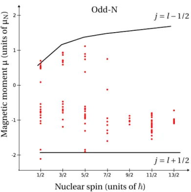
These values are known as the Schmidt limits or Schmidt moments. We show in Figure(2.1) the Schmidt diagrams, where the magnetic moment depends directly on the angular mo-mentum j . The full lines in these diagrams represent the Schmidt values for the magnetic moments as derived from Equation (2.15) by inserting the appropriate values for the g fac-tors. If we compare the experimentally determined magnetic moments, for nuclei having one valence nucleon, with Schmidt limits one can see that the experimental values always
Figure 2.1 – Schmidt diagrams for odd-neutron nuclei, as a function of angular momentum. The dots are the experimentally measured values.
are between and/or more or less on Schmidt limits, but do not coincide with them exactly. Even if the single particle model can account for the general dependence of the moments on j , its fails to explain why the observed values of moments do not coincide with those ob-tained by the single-particle model. In a real nucleus, the magnetic moment of nucleons are influenced by the presence of other nucleons and give a different value from the free nucleon hypothesis[2][3]. Therefore the single particle moment for a nucleon in a particular state can be calculated using effective single nucleon moments. Usually, effective g factor are used to provide a correction for missing interactions.
Let us now proceed to estimate the magnetic moment of two or more particle states outside an inert core. If we consider two particles with angular momenta I1and I2coupled to the
in-ert core with Icor e= 0. The total angular momentum is given by the sum of these two angular
momenta : ~I=~I1+ ~I2. If we substitute the total angular momentum I with relation Equation
(2.12) in Equation (2.11), we obtain:
where g1and g2are the g factors of the two nucleons. If the interaction between the two
par-ticles is neglected, the magnetic moment and g factor can be rewritten using the generalized Landé formula [4] as :
µ =〈IM|g1I1·~I+ g2I2·~I|IM〉M=I
I(I + 1) 〈IM|Iz|IM〉M=I, (2.17)
g =〈IM|g1I1·~I+ g2I2·~I|IM〉M=I
I(I + 1) . (2.18)
The evalution of the matrix element of ~I1·~I and ~I2·~I is performed as follow:
~I2= (~I 1+~I2)2= ~I21+ 2~I1·~I2+~I22, ~I1·~I2= 1 2(~I 2−~I2 1−~I 2 2), ~I1·~I = ~I1· (~I1+~I2) = ~I21+~I1·~I2. (2.19)
from which one can derive:
~I1·~I = 1 2(~I 2+~I2 1−~I21), ~I2·~I = 1 2(~I 2+~I2 2−~I22). (2.20)
Substituting this into Equation (2.18), we find:
g = g1[I(I + 1) + I1(I1+ 1) − I2(I2+ 1)]
I(I + 1) +
g2[I(I + 1) + I2(I2+ 1) − I1(I1+ 1)]
I(I + 1) , (2.21)
which can be written as:
g =1 2(g1+ g2) + 1 2(g1− g2) I1(I1+ 1) − I2(I2+ 1) I(I + 1) . (2.22)
This relation is called the additivity relation.
The second part of the Equation (2.21) vanishes when the two particles occupy two levels with same g factors. In that case, the g factor will be independent of the total spin.
2.2 The hyperfine interaction
The hyperfine interactions is defined as the interaction of the nuclear charge and current distribution of the nuclei with electromagnetic fields in its immediate surroundings. These
interactions influence the atomic and nuclear energy levels. At the atomic level, the magnetic dipole interaction between the nuclear moments and the fields induced by the electrons will give rise to the hyperfine splitting of the electronic states. The hyperfine interaction is de-fined as a coupling between the atomic spin~J to the nuclear spin~I and gives the total spin ~F =~I+~J, as shown in Figure(2.2).
At nuclear level as illustrated in Figure (2.3), the Zeeman splitting is induced by the
mag-Figure 2.2 – A schematic drawing illustrating a vector model of the free-ion hyperfine interaction.
netic dipole interaction with a magnetic field. This hyperfine interaction is observed in the response of the nuclear spin system to the internal electromagnetic fields of the medium or the applied electromagnetic fields.
Figure 2.3 – A schematic drawing illustrating the Zeeman splitings with a Larmor frequency ωL =
gµNB/~
is positioned on one of its regular lattice position, the magnetic substates m of a nucleus with a spin I remain degenerate.
The magnetic field within medium causes the rise of m-degeneracy of the nuclear energy levels. This field can be achieved by applying an external field, of the order of a few hundred Gauss up to sevral Tesla, or via the hyperfine magnetic field of a host material, of the order of ten to hundred Tesla [5].
The interaction of the nuclear magnetic momentµ with a static magnetic field ~B is de-fined by the Zeeman Hamiltonian [6]:
HB= −~µ ·~B = −
gµN
~ ~I·~B = −ωL
IZ, (2.23)
withωL= g µNB/~being the Larmor frequency and g is the nuclear g factor. The magnetic
field ~B is defined in a reference frame with the z-axis (~B = B~ez). The energy splitting of the
Zeeman levels is propotional to m as defined in Equation (2.24). The substates of m of the spin operator are eigenstates of the Zeeman Hamiltonian.
Em= −~ωLm. (2.24)
The Zeeman splitting levels are equidistant and propotional to the Larmor frenquency. As a descriptive picture, the splitting can be visualized as a precession of the spin I around the magnetic field direction ~B with a Larmor frequencyωL.
2.3 Nuclear spin orientation
During any nuclear reaction mechanism, a spin-oriented ensemble of the nuclear states is formed to a preferential direction in space, the |Im〉 states are unequally populated. To study a spin-oriented ensemble, we deal with the angular distribution ofγ-rays emitted from oriented states which are formed by nuclear reactions and also with particle-γ angular corre-lations. Usually, the measurement ofγ-rays distributions and particle-γ correlations are used to assign the multipolarities of theγ-rays transitions, and therefore the spin of excited states. They also allow to estimating the mixing ratios of mixed multipolarityγ-ray transitions. But, one needs enough orientation in the excited state of interest to be able to distinguish between
different multipolarity transitions [7].
Let us consider a system of three groups, the original oriented state is denoted as I0, the initial
and final states are denoted as Ii and If, respectively. The initial oriented state is usually
de-scribed by the orientation parameter Bk, however, if the orienting interaction lacks axial
sym-metry, it can be described by the general statistical tensorsρkq (See section2.3.1.1). In the
case of unobserved radiations between the I0and Ii, the orientation of the Ii is determined
by a modification of I0with de-orientation coefficients Uk(See2.3.1.4). In other hands, if the
intermediate states between I0and Ii are sufficiently long lived, a perturbation of the
angu-lar distribution can take place by modification of the orientation by the direct interaction of the electromagnetic moments of that state with the nuclear environment. The perturbation coefficients are represented as Gk (See section2.3.2.1).
2.3.1 Angular distribution of
γ-rays
The angular distribution of a radiation emitted by an oriented state ensemble of Iiis given
using the following expression:
W(θ,φ) =p4πp 2Ii+ 1 X k,q ρkq(Ii)AkYkq(θ,φ) p 2k + 1 , (2.25)
whereρkq(Ii) are statistical tensors, Akare the angular distribution coefficients and Ykq(θ,φ)
are the spherical harmonics and the anglesθ and φ are the direction of emission of the radi-ation.
In the case of an axially symmetric oriented state, Equation (2.25) is reduced to the most frenquently used form of the angular distribution at an angleθ with respect to the beam axis and has the form [8]:
W(θ) = X
k,q
Bk(Ii)AkPk(cosθ). (2.26)
The Bkcoefficients are orientations parameters which depend on spin of the initial state
to which the nucleus is excited, Ii. The angular distribution coefficients Ak depend on Ii,
If and the multipolarity, which may be pure or mixed. The Pk(cosθ) are the Legendre
Pk(cosθ) are symmetric about θ = 90◦. Hence, the angular distribution is valid only for even
values of k.
2.3.1.1 Statistical tensors
The non-axially symmetric orientation of the initial state is described by using the density matrix, which is propotional to the statistical tensor. The density matrix formalism is:
ρmm0= 〈m|ρ|m0〉 , (2.27)
where m is the projection of the nuclear spin Ii on a z-axis. Using the density matrix, a
statistical tensor is given by the formula [9]:
ρkq= p 2Ii+ 1 X m,m0 (−1)Ii+m0 Ii k Ii −m0 q m 〈m|ρ|m0〉 , (2.28) Ii k Ii −m0 q m
: is the Wigner 3-j symbols.
If the spin has an axial symmetric orientation with respect to a chosen coordinate frame (ZOR axis), only the q=0 components ofρkq are non-zero and the non-diagonal elements
define the coherence between the different m-states. Using the diagonal elements of the density matrix as population parameters P(m) with m = m0implies that the Equation (2.28) becomes : ρk0= p 2Ii+ 1 X m (−1)Ii+m Ii k Ii −m 0 m P(m). (2.29)
The statistical tensorρkq is related to the orientation parameters Bkqby:
ρkq= Bkq p 2k + 1, (2.30) where Bk0= p 2Ii+ 1 p 2k + 1X m(−1) Ii+m Ii k Ii −m 0 m P(m). (2.31)
To sum up, Bkqare related to the distribution of the magnetic substates of a nucleus in an
ex-cited state with spin Ii oriented around a chosen coordinate frame (z-axis). The distribution
of magnetic substate can be specified by the population P(m) of the 2Ii+ 1m substate [10],
which are related to the amount of alignment in the excited state.
Due to their simple transformation under rotation, one can use the orientation tensor to transform the f 1 frame into the f 2 frame:
Bkqf 2=X
Q
BkQf 1DkqQ(α,β,γ), (2.32)
where DkqQare Wigner D-matrices and (α,β,γ) are Euler angles.
2.3.1.2 Alignment and polarization
In the case where all spins are pointing to random directions, the ensemble of spins show an isotropic distribution. The m-quantum states, which are the spin projection on the orien-tation axis, are equally populated.
P(m) = 1 2Ii+ 1
for all m ; Bk= 0(k 6= 0) (2.33)
However, if all spins are pointing one direction, we talk about an axially symmetric en-semble of spins. Two kinds of axially symmetric enen-sembles are defined as an aligned and polarized ensemble. The alignment produced in an excited state in the nucleus shows a re-flection symmetry of all m-quantum states populations which are the spin projected states on the axial symmetry axis zOR, which means that P(m) = P(−m).
P(m) = P(−m);Bk= 0 for odd k (2.34)
This case has two different types. If the angular momentum of the nucleus is aligned per-pendicular to the symmetry axis zOR, then the preferential population of the m = 0 substate
dominates and the alignment is named as oblate alignment (Bk< 0). If the angular
momen-tum of the nucleus is aligned parallel and anti-parallel to the symmetry axis zORthen the m
= ±Ii substates are preferentially populated and the alignment is referred to as prolate
When, the reflection symmetry is broken, the ensemble is called as polarized and it is de-scribed as:
P(m) 6= P(−m);Bk6= 0 for odd k (2.35)
-2 -1 0 +1 +2 m -2 -1 0 +1 +2 m -2 -1 0 +1 +2 m
Zor Zor Zor
Polarization Oblate alignment
Prolate alignment
P(m) P(m) P(m)
Figure 2.4 – Schematic drawing of different types of nuclear spin orientation (Prolate, oblate alignment and polarization)
The degree of normalized alignment, A, is defined as:
A ≡ P mα2(m)P(m) |α2(max)| = P m(Ii(Ii+ 1) − 3m2)P(m) |α2(max)| , (2.36)
whereα2(m) = Ii(Ii+ 1) − 3m2[12]. The value of the normalization depends on whether the
alignment is oblate (A < 0) or prolate (A > 0).
If A = −1 means that the ensemble is oblate-aligned. When the states of ensemble are given with integer spins, the dominant population is in the m = 0 substates. One can see this align-ment in fast-fragalign-mentation reactions. For oblate-aligned half-integer spins, the population is equally distributed in the m = ±1/2 substates. Thus α2(max) for full oblate alignment is:
|α2(m = 0)| = Ii(Ii+ 1) for integer spin,
|α2(m = ±1/2)| = Ii(Ii+ 1) − 3/4 for half-integer spin.
(2.37)
For prolate alignment A = +1, only the magnetic substates with m = ±Ii are populated. Then
theα2(max) for full prolate alignment is:
|α2(m = ±Ii)| = I(2I − 1) for any spin. (2.38)
In practice to refer to the alignment, one can define the alignment in terms of Bk with k = 2,
with the k = 2 term. The alignment is then related to the k = 2 orientation tensor as follows:
A = p
I(I + 1)(2I + 3)(2I − 1) p
5|α2(max)|
B2. (2.39)
The nuclear polarization is defined in terms of the k = 1 orientation tensor. The normalized polarization is defined as:
P = P
mmP(m)
I , (2.40)
and the relation between the polarization and k = 1 orientation tensor is:
P = − s
I + 1
3I B1. (2.41)
2.3.1.3 The distribution coefficients
The angular distribution coefficients Ak(Ii− > If) are described by the formula:
Ak=
1
1 + δ2[Fk(L, L 0, I
f, Ii) + 2δFk(L, L0, If, Ii) + δ2Fk(L, L0, If, Ii)]. (2.42)
Where the mixing rationδ is defined as:
δ =〈If||π(L + 1)||Ii〉 〈If||π0(L)||Ii〉
, (2.43)
whereπ and π0specify the type of radiation, electric or magnetic. Thus, the angular distribu-tion coefficients Akdepends on the transition multipolarity.
However, the Akare insensitive to the character of the transition for pure multipole
tran-sitions and it is not possible to determine the parity of the nuclear states of interest. In other words, if the Ak coefficients depend on the multipole mixing rationδ, therefore, the parity
information can be obtained.
The Fkcoefficients in Equation (2.42) are defined as:
Fk(L, L0, If, Ii) = (−1)If+Ii+1 p (2k + 1)(2L + 1)(2L0+ 1)(2Ii+ 1) × L L0 k 1 −1 0 L L0 k Ii Ii If (2.44) where the L L0 k 1 −1 0
is a Wigner 3-j symbol, and L L0 k Ii Ii If is a 6-j symbol.
For a pure multipole transition, e.g. a pure E2 transition, L = L0= 2. The F-coefficients are tabulated in the Ref [13].
2.3.1.4 The deorientation coefficients
If there are one or more unobserved radiations between the oriented parent state I0and
the intermediate state Ii, the orientation of the Ii is determined by a modification of I0with
deorientation coefficients Uk. Therefore, the orientation of the state Ii will be less than the
parent state I0. The orientation tensors of the intermediate state Ii in the cascade becomes
[8]:
Bkq= Uk(I0→ Ii)Bkq(I0). (2.45)
For a pure transition of multipole order L, emitted between I0and Ii, the deorientation
coef-ficient is given by:
Uk(I0, Ii, IL) = (−1)I0+Ii+k+L p (2I0+ 1)(2Ii+ 1) I0 I0 k Ii Ii L . (2.46)
For the mixed multipolarity L and L + 1 between levels of spin I0 and Ii, the dorientation
coefficients becomes:
Uk(I0→ Ii) =
Uk(I0, Ii, IL) + δ2Uk(I0, Ii, L + 1)
1 + δ2 . (2.47)
2.3.2 Perturbed angular distribution of
γ-rays
In general the perturbed angular distribution of radiation emitted from an axially sym-metric oriented states can be expressed by:
W(θ,t) = X
k
BkGkk(t )AkPk(cosθ), (2.48)
where Ak are the angular distribution coefficients, Bk are the orientation coefficients, Gkk
are perturbation factors, and Pk(cosθ) are the Legendre polynomials. The angle θ gives the
direction of observation of the radiation emitted with respect to the symmetry axis z of the oriented state, often the beam direction.
2.3.2.1 The perturbation coefficients
The perturbations are provoked by the interaction of nuclear moments with the electro-magnetic fields in the medium. They depend mainly on the nuclear moments of the state Ii, the electromagnetic fields of the nuclear environment and the lifetimesτ of the state Ii.
Interaction of nuclear dipole moment with a static magnetic field can modify the m-state populations and thus affect the angular distribution of the subsequentγ-rays.
The perturbing Hamiltonian K is assumed to be a static Hamiltonian. The spin orientation of the state Ii evolves with time under the influence of K. The time evolution of the statistical
tensors can be evaluated with the time evolution of the density operator:
i~∂ρ(t)
∂t = [K, ρ(t )], (2.49)
which is known as the Von Neumann equation. The solution is:
ρ(t) = e−i Kt /~ρ(0)e+i Kt /~. (2.50)
The time evolution of the statistical tensors is described by the perturbation coefficients:
ρk q(Ii, t ) = X kq ρk q(Ii, 0)Gq q kk(t ). (2.51)
The perturbation coefficients describe the influence of the extra-nuclear on the orientation of the nuclear state Ii and are given by [14]:
Gq q kk(t ) = q (2k + 1)(2k + 1)X mm (−1)m−m Ii Ii k −m m0 q × Ii Ii k −m m0 q 〈m|e−i Kt /~|m〉 〈m0|e+i Kt /~|m0〉 . (2.52)
2.3.2.2 Spin-oriented ensemble pertubed by the static magnetic interactions
Producing a spin-oriented ensemble of excited nuclear states Ii by a suitable reaction is
the first step, in order to measure a magnetic dipole momentµ. This ensemble can be per-turbed with a magnetic field, either an external one or hyperfine field, which causes a pre-cession of the spin-oriented ensemble with Larmor frequencyωLaround the magnetic field
direction. If the magnetic of the interacting field ~B is known, the g factor can be extracted fromωL. On the other hand, if the nuclear g factor is known, the magnetic field at the site of
nuclei can be determined.
When the perturbation of the ensemble is caused by the interaction with an external mag-netic field, the perturbation coefficients can be described classically. If the symmetry axis is
chosen to the z-axis of the SK system and the Hamiltonian K is diagonal, the perturbation
coefficients of Equation (2.52) become:
Gq q kk(t ) = q (2k + 1)(2k + 1)X mm Ii Ii k −m m0 q × Ii Ii k −m m0 q × e−i (Em−Em0)t /~, (2.53)
where Em are the eigenvalues of K. The magnetic splittings of the state Ii are uniform:
Em− Em0= (m − m0)~ωL= q~ωL, (2.54)
and q = m −m0is fixed. The perturbation coefficients are reduced by using the orthogonality of the 3 − j symbols to give the form:
Gq q
kk(t ) = e
−i ωLtδq qδkk. (2.55)
2.3.3 Particle-
γ angular correlation
Consider now that the state Ii decays to state If by th emission ofγ-ray at the spherical
polar and azimuthal detection angles, respectively,θγ andφγin coincidence with a particle at the spherical polar and azimuthal detection angles, respectively,θp andφp. The beam
axis is the z axis in the coordinate system used. Theθγ andθp are measured with respect
to the beam axis. ∆φ = φγ− φp is the difference between the azimuthal detection angles of
the particles andγ-rays. Thus, the angular correlation function has the form and references therein [10]:
W(θp,θγ,∆φ,t) = X
kq
akq(θp)Gk(t )Dk∗q0(∆φ,θγ, 0). (2.56)
With akq(θp) = Bkq(θp)QkFk. The Bkq(θp) is the statistical tensor in (2.31), which is
deter-mined by the segmented particle detector’s position. Fk represents the F−coefficient for the
γ-ray transition in Equation (2.44), and Qk is the attenuation factor for the finite size of the
γ-ray detector (see AppendixA.1.1). The Dk∗q0(∆φ,θγ, 0) is the Winger-D matrix (see Appendix A.1.2). The Gk is the attenuation coefficient. For an example of E2 excitation, k = 0,2,4 and
−k6q6k. The sum above is only valid for even k values. For the k odd values the statistical tensor are zero due to the parity conservation symmetry of the electomagnetic interaction.
2.3.3.1 Attenuations coefficients
The time-dependent vacuum de-orientation effect is specified by the attenuation coeffi-cients, Gk(t ). For H-like J = 1/2 configurations the Gk(t ) are cosine functions[10]:
Gk(t ) = 1 − bk(1 − cosωLt ), (2.57)
where t is the mean life of the nuclear state, and bkis written:
bk=
k(k + 1)
(2I + 1)2. (2.58)
TheωLis the Larmor frequency which is determined by the nuclear g factor
ωL= g (2I + 1)µN
~ B1s' g (2I + 1)800Z 3
MHz. (2.59)
The B1sis the hyperfine field at the nucleus due to a 1s electron:
B1s= 16.7Z3R(Z)Tesla. (2.60)
with the relativistic correction factor:
R(Z) ' [1 + (Z/84)2.5]. (2.61)
2.4 Techniques to orient nuclei and their applications
It is necessary to produce a spin-oriented ensemble of excited nuclear state, in order to measure the nuclear moment. From a suitable reaction mechanism and nuclear spin inter-action with surrounding environment, after the production of the nuclear state, the spin-oriented nuclear ensemble can be produced with some degree of orientation which depends on the formation process and reaction mechanism.
The orientation methods differ with the different reaction mechanisms. Usually, the polar-izations methods used experimentally are optical pumping, low temperature nuclear ori-entation, tilted foil and projectile fragmori-entation, while alignment methods are related to the reaction mechanisms such as fusion evaporation, direct transfer reactions, incomplete fusion reactions, multinucleon transfer reactions, projectile fragmentation, knock-out and intermediate-energy Coulomb excitation, etc.
The optical pumping is described as the hyperfine interaction between the electron spin J and the nuclear spin I [15]. The atomic spin is polarized after several excitation/decay pro-cesses of photons and transfers this polarization to the nuclear ensemble which can be po-larized of typically 30-50%. Where, the low temperature nuclear orientation method [16] is based on the interactions of nuclear electromagnetic moments with very strong electromag-netic fields at very low temperature (mK). Because of the large Zeeman spliting and the low temperature of the environment, the Boltzmann distribution of the nuclear spins have the non-degenerate m-quantum states. Therefore, the nuclear spins become polarized. From this technique, the typical amounts of polarization that can be observed are of the order of 20-80%. In another technique which is named Titled Foils (TFT), when an atom passes through a thin foil that is tilted with respect to the beam direction, the electron spins of the ions leaving the foil become polarized. This polarization is transferred to the nuclear spin via the hyperfine interaction in flight in vacuum after polarization of the ensemble when passing through the foil surface. One can place a several foils after each other at well defined distance to increase the nuclear polarization.
Another simple way to get a spin-oriented ensemble of nuclei is via the spin-orientation pro-duced during the reaction itself.
2.4.1 The spin-oriented ensemble in fusion-evaporation reactions
In fusion-evaporation reactions, the spin alignment of the excited states, including iso-mers, can be described by a Gaussian distribution function:
P(m) = e
−m2/2σ2
P
n=Iie−n
2/2σ2. (2.62)
The width of the Gaussian distribution,σ, is related to the amount of alignment in the excited state. The orientation mechanism in fusion-evaporation reactions is illustrated by the large orbital angular momentum of the projectile ions which produce compound systems which have strong alignment of their angular momenta in the plane perpendicular to the beam di-rection. The rapid decay of these highly excited compound systems, by neutron and gamma emission, leaves the angular momentum vector of the populated states still strongly aligned, thus causing considerable anisotropies in the angular distributions of theγ-rays de-exciting the excited states. Using this kind of reaction mechanism allow to obtain a spin alignment
of states typically between 25% and 75% and a spin polarization up to 40% [9], when the re-action products are selected at an angle with respect to the incoming beam. However this type of production mechanism is not suitable to produce neutron-rich nuclei lying far from the stability line. Therefore, one can not consider this reaction mechanism to investigate iso-meric states for neutron-rich nuclei. Other reactions can be applicable with radioactive ion beams (RIB) and, at the same time, provide sufficient degree of spin orientation.
2.4.2 The spin-oriented ensemble in Direct transfer reactions
The Direct transfer or single-neutron transfer reactions have been demonstrated to be widely applicable for the population of excited states using radioactive beams. The degree of 13% spin alignment was obtained with stable beam and reaction65Cu(d,p)66mCu [17] and
65Ni(d,p)65mNi [18]. Although the production yield of exotic nuclei is higher in
intermedi-ate and high-energy projectile-fragmentation reactions (See section 2.4.4), the low energy transfer reactions show a higher level of spin-orientation. On the other hand, several dif-ficulties oppose to the application of single-nucleon transfer reactions for nuclear moment studies of isomeric states with radioactive beams. The main difficulty comes from the en-ergy/momentum transfer between the projectile and target nuclei for single-nucleon trans-fer reactions, which is relatively small. This does not allow for an efficient separation between projectile that needs to go away from the target, and the reaction products that need to re-main in the target. Therefore the single-nucleon transfer reaction is not a simple production mechanism to use for isomeric-states studies with RIB.
2.4.3 The spin-oriented ensemble in incomplete fusion reactions
In the case of incomplete fusion, sometimes is called multinucleon transfer reactions, the energy/momentum transfer between the projectile and target nuclei can be large. The incomplete fusion processes are described to take place around the Coulomb barrier. When the incident energy of the projectile in the center of mass frame is sufficient to vanquish the Coulomb barrier, then the incident ion fuses with the target nucleus to form a composite system. As we can imagine, the projectile comes near the field of the target nucleus, it may break up and one of the fragments may fuse. One can cite several advantages of the
incom-plete fusion, one of these advantages is the population of higher spin, a few reaction channels opened and change of Z between the beam and the products. In order to reach to the neu-tron rich side of the nuclear chart, two reaction channels7Li(64Ni,α n)66mCu and7Li(64Ni,α p n)65mNi were performed at the ALTO facility in Orsay, France in December 2013 [19]. The results from this experiment are discussed in details in this reference (See section4.1).
In fellowing works [20][21], it is shown that in multinucleon transfer reactions of neutron-rich Ca isotopes, with using the48Ca beam on64Ni at energies approximately twice the Coulomb barrier, the maximum alignment is of the order ' 70% perpendicular to the reaction plane. This can be used in determination of spin and parity of the neutron-rich nuclei which are hard to reach by standard fusion-evaporation reactions.
2.4.4 The spin-oriented ensemble in projectile-fragmentation reactions
Projectile fragmentation can be described as a peripheral collision between the projec-tile and a target nucleus. In this reaction mechanism the spin-orientation is described by the participant-spectator model1or, more commonly, the abrasion-ablation model. More details can be found at this reference [22]. In the participant-spectator model, the spin ori-entation of the fragments results from the orbital angular momentum left in the fragments during the projectile-target interaction, named also abrasion stage. The general principle is first suggested by Asahi et al. [23] [24]. When a projectile with an initial momentump~0
col-lides with the target, a participant part of nucleons at the position ~R0with momentump~nis
removed from the projectile. Thep~nis the sum of momenta of the removed nucleons. Thus
the nuclear spin ~IPFof the fragments is given with respect to the centre of mass as:
~
IPF= ~R0× ( ~pn) (2.63)
Using the momentum conversation in the projectile-rest frame, the momentump~PF of the
fragment can be written asp~PF=p~0− ~pn. Thus the orientation of the spin is determined as a
function of the momentump~PF:
~
IPF= ~R0× ( ~p0− ~pPF) (2.64)
1. The "participant" zone is consists of highly excited prefragments. The outer projectiles which are called “spectators” are only slightly affected by the collision.
The resulting spin orientation produced in the projectile fragmentation reaction is partially or completely attenuated because of the removal of nucleons from the projectile.
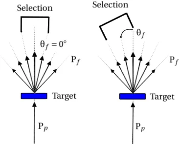
Figure 2.5 – Schematic drawing of the fragment selection. On the left side, the selected fragments (θf = 0◦) are spin aligned, where, on the right side the fragments selected under an angleθf with respect to the primary beam direction are spin polarized (right).
If the fragments produced in an intermediate or high-energy projectile fragmentation re-action are selected symmetrically around angle 0◦with respect to beam direction, the frag-ment spins are spin aligned (see Figure2.5). If fragments are selected at a finite angle with respect to the primary beam direction, the fragments are spin-polarized (see Figure2.5). The amount of alignment produced in fragmentation reactions varies considerably between 5% and 35% due to a range of experimental conditions.
2.4.5 The spin-oriented ensemble in Coulomb excitation reactions
The Coulomb force between a projectile of radius rp with a mass Apa nuclear charge Zpe
and a target nucleus of radius r2with mass At charge Zte is : ZpZte2/r2, where r = rp+ rt =
r0(A1/3p + A1/3t ) with r0= 1.25 fm is the average nucleon radius. The distance of the target from
the asymptote of the hyperbola is called the impact parameter (See Fig2.6). If the reduced de Broglie wavelengthňof the incoming particle is sufficiently short than the half-distance of