Smoothing algorithms for mean-flow extraction in large-eddy simulation of complex turbulent flows

(1)

HAL Id: hal-00566009

https://hal.archives-ouvertes.fr/hal-00566009

Submitted on 11 Jun 2012

HAL is a multi-disciplinary open access

archive for the deposit and dissemination of

sci-entific research documents, whether they are

pub-lished or not. The documents may come from

teaching and research institutions in France or

abroad, or from public or private research centers.

L’archive ouverte pluridisciplinaire HAL, est

destinée au dépôt et à la diffusion de documents

scientifiques de niveau recherche, publiés ou non,

émanant des établissements d’enseignement et de

recherche français ou étrangers, des laboratoires

publics ou privés.

Smoothing algorithms for mean-flow extraction in

large-eddy simulation of complex turbulent flows

Adrien Cahuzac, Jérôme Boudet, Pierre Borgnat, Emmanuel Lévêque

To cite this version:

Adrien Cahuzac, Jérôme Boudet, Pierre Borgnat, Emmanuel Lévêque. Smoothing algorithms for

mean-flow extraction in large-eddy simulation of complex turbulent flows. Physics of Fluids, American

Institute of Physics, 2010, 22, pp.125104. �10.1063/1.3490063�. �hal-00566009�

(2)

Smoothing algorithms for mean-flow extraction in large-eddy simulation

of complex turbulent flows

A. Cahuzac,1,a!J. Boudet,1,b!P. Borgnat,2,c!and E. Lévêque2,d!

1

LMFA, École Centrale de Lyon, Université de Lyon, CNRS, 36 Avenue Guy de Collongue, 69134 Ecully Cedex, France

2

Laboratoire de Physique, ENS de Lyon, Université de Lyon, CNRS, 46 allée d’Italie, 69364 Lyon Cedex 07, France

sReceived 18 February 2010; accepted 20 August 2010; published online 14 December 2010d Based on physical arguments, the importance of separating the mean-flow from turbulence in the modeling of the subgrid-scale eddy-viscosity is emphasized. Therefore, two distinct time-domain smoothing algorithms are proposed to estimate the mean-flow as the simulation progresses, namely, an exponentially weighted moving average sor exponential smoothingd and an adaptive low-pass Kalman filter. These algorithms highlight the longer-term evolution or cycles of the flow but erase short-term fluctuations. Indeed, it is our assumption that the mean-flowsin the statistical sensed may be approximated as the low-frequency component of the velocity field and that the turbulent part of the flow adds itself to this “unsteady mean.” The cutoff frequency separating these two components is fixed according to some characteristic time-scale of the flow in the exponential smoothing, but inferred dynamically from the recent history of the flow in the Kalman filter. In practice, these two algorithms are implemented in large-eddy simulations that rely on a shear-improved Smagorinsky’s model. In this model, the magnitude of mean-flow rate of strain is subtracted from the magnitude of the instantaneous rate of strain in the subgrid-scale eddy-viscosity. Two test-cases have been investigated: a turbulent plane-channel flowsRew= 395d and the flow past a circular cylinder in the subcritical turbulent regimesReD= 4.73 104_{d. Comparisons with direct numerical simulation and}

experimental data demonstrate the good efficiency of the whole modeling. This allows us to address nonhomogeneous unsteady configurations without adding significant complication and computational cost to the standard Smagorinsky’s model. From a computational viewpoint, this modeling deserves interest since it is entirely local in space. It is therefore adapted for parallelization and convenient for boundary conditions. © 2010 American Institute of Physics.

fdoi:10.1063/1.3490063g

I. CONTEXT AND MOTIVATIONS

Large-eddy simulation sLESd is a promising technique that offers an affordable means for the numerical simulation of turbulent flows.1,2Unlike the Reynolds-averaged Navier– Stokes methods commonly used in the industry, LES gives a direct representation of the large-sized turbulent eddies and their dynamics. It is therefore expected to provide a better description of turbulence impacts. LES has already demon-strated its capabilities in computations of academic building-block flows; however, further progress is still required to address realistic complex configurations.3 The present work aims at improving this situation. Our guideline is to develop numerical modeling that remains as simple as possible in its formulation but captures the “basic physics,” therefore offer-ing an interestoffer-ing compromise between accuracy and com-putational cost.

Turbulence that occurs in nature, or in engineering ﬂows, is usually not, even approximately, homogeneous. There are frequent variations of the mean velocity with

po-sition sand time in unsteady conﬁgurationsd. In the follow-ing, the general framework of LES is brieﬂy recalled and physical arguments are brought forward to justify the impor-tance of the mean velocity gradients in the modeling of the subgrid-scalesSGSd eddy-viscosity.

LES is rooted in the idea to discretize the flow on a grid whose resolution is coarse compared to the size of the small-est turbulent eddies. Therefore, only the large-sized eddies are represented numerically. This is justifiable since the large-sized eddies contain most of the kinetic energy and their strengths make them the efficient carriers of momen-tum, heat, mass, etc. On the contrary, the small-sized eddies are mainly responsible for dissipation and contribute little to transport. Conceptually, the solution of a LES is expected to represent the flow variables filtered over a “filter window” whose characteristic width corresponds to the grid reso-lution. These filtered variables are solutions of the flow equa-tions supplemented by terms accounting for the action of the sunresolvedd SGS fluctuations on the grid-scale dynamics.4

These additional terms need to be modeled in order to close the governing equations, which constitutes a major difﬁculty in the case of complex turbulent ﬂows.

In the present study, primarily devoted to weakly com-pressible aerodynamics, the relevant ﬂow variables arer,ru,

ad_{Electronic mail: adrien.cahuzac@ec-lyon.fr.} bd_{Electronic mail: jerome.boudet@ec-lyon.fr.} cd_{Electronic mail: pierre.borgnat@ens-lyon.fr.} dd_{Electronic mail: emmanuel.leveque@ens-lyon.fr.}

(3)

andretreferring to the mass, momentum, and total energy of the fluid per unit volume, respectively. The related filtered variables are ¯,r ru_;¯ur˜ , and ret;¯er˜ , where the overbart refers to the grid filter operator and the tilde is the Favre operatorsq˜ =rq /¯rd. The filtered flow equations are expressed as ]r¯ ]t + ]s¯ur˜jd ]x_j = 0, s1d ]s¯ur˜id ]t + ]s¯ur˜ ui˜jd ]xj = −]P ¯ ]xi +]t¯ij ]xj +]Pij SGS ]xj , s2d ]s¯er˜td ]t + ]fs¯er˜ + Pt ¯ du˜jg ]xj =]fui˜s¯tij+ Pij SGS dg ]xj + ] ]xj

S

l ¯]˜T ]xj

D

−]Qj SGS ]xj . s3d

Implicit summation on repeated indices is used. The ﬂuid is air, considered as Newtonian with constant dynamic viscos-itym¯ = 1.83 10−5 _{kg m}−1_s−1_, t ¯_ij=m¯

S

]u˜i ]xj +]u˜j ]xi −2 3 ]u˜k ]xk dij

D

, s4d

and constant thermal conductivity ¯ =2.54l

3 10−2 _{W m}−1_K−1_{. Air is assumed to behave as a perfect}

gas, thus following P

¯ = r¯Tr˜ with r = 287 J kg−1K−1, s5d where P is the pressure and T is the temperature. The ratio of speciﬁc heats sat constant pressure and volumed is ﬁxed at

g= Cp/_C

v= 1.4. The SGS stress tensor sPij

SGS

d and the SGS heat currentsQj

SGS

d encompass the exchanges of momentum and heat with the SGS motions. A common thread is to as-sume that these terms are essentially responsible for a diffu-sive transport at grid scale. This assumption yields

P_ijSGS=mSGS

S

]u˜_i ]x_j+ ]u˜_j ]x_i− 2 3 ]u˜_k ]x_kdij

D

and s6d QSGS_j =−mSGSCp PrSGS 3 ]T ˜ ]xj ,

wheremSGSrepresents a SGS eddy-viscosity and PrSGS= 0.9

may be viewed as a fixed SGS Prandtl number.5 Unlike the molecular viscosity, the eddy-viscosity is a property of the flow but not of the fluid. It is therefore expected to depend explicitly onsresolvedd flow variables and on the local grid spacing.

In practice, the eddy-viscosity is primarily intended to ensure the correct drain of kinetic energy from the resolved to the unresolved turbulent scales. Tackling this problem from a deterministic viewpoint is mainly out of reach.6 A statistical approach is rather adopted and an expression of the eddy-viscosity is sought on the basis of statistical hypotheses

made on the SGS turbulent scales.7Along this line, physical arguments are now provided to defend the importance of mean-ﬂow gradients in the SGS properties.

Despite the nonhomogeneous nature of most turbulent ﬂows, it is commonly thought that the small-scale properties of turbulence should be considered as locally homogeneous sand isotropicd. This hypothesis relies on the idea that small-sized eddies adjust themselves via strong nonlinear in-teractions, in which all statistical information about the large-scale inhomogeneities is lost. This is the classical phe-nomenology of Kolmogorov’s theory.8Within this picture, it is implicitly assumedsbut often forgottend that the size of the turbulent eddies should be small compared to the length-scale associated with the mean velocity gradients, which is

Ls, u

₈

S, s7d

where u

₈

;

Î

kuu

₈

u2_{l and S ;}

Î

_u¹kulu2_{denote the norms of the}

ﬂuctuating velocity and of the mean velocity gradient, re-spectively. Here, angular brackets a priori refer to an en-semblesstatisticald average and the ﬂuctuating velocity arises from the Reynolds decomposition: u =kul + u

₈

. The charac-teristic scales7dis obtained by equaling the time-scale asso-ciated with the mean velocity gradientscharacteristic of the mean-ﬂow distortiond and the turn-over time of turbulent ed-dies of size ,scharacteristic of turbulent interactions at scale ,_{d. That is, 1 / S , «}−1/3_,2/3

for , = Ls, according to

Kolmog-orov’s theory.8 From the averaged Navier–Stokes equations, the mean dissipation rate sper unit massd « = −kui

8

u

8

jl 3]kuil /]xj, u

8

2S, which ﬁnally yields Ls, u

8

/S or,

equivalently,9 Ls,

Î

« / S3. Note that the previous reasoning

relies on dimensional arguments that ignore dimensionless factors. In that sense, the symbol “,” should be understood as “is of the order of.” In the jargon of ﬂuid mechanics, S is usually referred to as the shear and Ls is the shear

length-scale. The shear is often expressed as S =

Î

2kSijlkSijl,

wherekSijl is the rate-of-strain tensor of the mean-ﬂow. Turbulent eddies of size smaller than Ls evolve rapidly

enough and are insensitive to the mean-flow distortion: The mean-flow acts principally to convect these eddies without significantly stretching them. On the contrary, turbulent ed-dies of size larger than Lshave no time to adjust dynamically

while they are distorted by the mean-ﬂow gradients. Termed differently, the shear length-scale Ls isolates the problem of

the self-interaction of ﬂuctuating velocities, at scales , , Ls,

from the problem of the interaction of the ﬂuctuating veloc-ity with the mean-ﬂow velocveloc-ity, at scales , . Ls. This feature

is of great importance in the context of LES, as it implies that the statistical properties of the SGS motionsand there-fore the nature of the SGS eddy-viscosityd should differ de-pending on whether the grid resolution D is locally smaller, or larger, than the shear length-scale Ls. Therefore, it is

de-sirable to account explicitly for the mean-ﬂow gradients in the modeling of the SGS eddy-viscosity, also the canonical assumption of homogeneous and isotropic turbulenceswhich ignores the mean-ﬂow inhomogeneities: S. 0 and Ls. `d

(4)

should be abandoned. This is particularly relevant for high-Reynolds-number flows, when the resolution of the simula-tion is almost comparable to the large scales of the flow. These features naturally call for a generic procedure to esti-mate numerically the mean-flow and evaluate the SGS eddy-viscosity as the LES progresses. This is the main concern of the present study, which will be developed in Sec. II. Prac-tical implementations in LES relying on a shear-improved Smagorinsky’s model will be examined in Sec. III.

II. SMOOTHING ALGORITHMS FOR MEAN-FLOW EXTRACTION

Statistical ensemble average may be approximated by space average over directions of homogeneity, whenever it is possible. When it is not, time average may be used instead. Space average is relevant to simple-geometry flows swith directions throughout which fluctuations can be considered as statistically homogeneousd, whereas time average is ad-equate when the flowsits mean and its fluctuationsd remains statistically stationary in time. In the presence of determinis-tic unsteadiness, such as vortex shedding or blade passing in a turbomachine, these two approximations must clearly be abandoned. Therefore, a more general procedure must be de-signed to extract the mean velocity field and track its pos-sible evolution sif large-scale instabilities develop in the flowd.

Our proposal is based on weighted moving average in time, which may be viewed as a generic smoothing operation that highlights longer-term variations or cycles but erase rapid fluctuations. It is here assumed that the mean-flow is given sat each grid pointd by the low-frequency component of the velocity field, and that the turbulent component of the flow adds itself to this “unsteady mean.” From the viewpoint of signal-processing, extracting a low-frequency trend from a time series is a “dangerous technique” that requires to deter-mine a priori a cutoff frequency above which excitations should be ignored. This cutoff frequency is well defined if there exists a clear-cut separation in the power-spectrum of the signal so that a low-frequency component may be iso-lated from the high frequencies. Also, it assumes that the separation between the mean-flow and such fluctuations is stationary. In the context of turbulent flows, there is no clear separation in frequency, as fluid dynamics is known to ex-hibit large-band spectra,5 and steadiness is not always achieved either. Nevertheless, strategies have been elabo-rated in order to extract low-frequency trends from the ve-locity time series. These trends are assumed to be represen-tative of the mean-flow behavior, even if they unavoidably include some turbulent low-frequencies as well.

Two distinct algorithms are considered, based on exist-ing well-known smoothexist-ing schemes. They are presented in detail and discussed in relation to their application to mean-ﬂow extraction. First, we introduce an exponentially weighted moving average susually called exponential smoothingd with a ﬁxed smoothing factor, hence a stationary method. This basic method should be considered as a base-line approach, a starting point for comparisons with more elaborated smoothing methods. Then, an adaptive Kalman

ﬁlter is presented as a reﬁnement of the exponential smooth-ing. This second approach does not require an a priori stated value for the cutoff frequency but only the prescription of a relevant interval for this frequency; the cutoff frequency adapts itself dynamically within this interval according to the recent history of the signal. These two methods are now presented.

A. Exponentially weighted moving average

A simple method for extracting the low-frequency com-ponent of the velocity field would be a movingsunweightedd arithmetic average of the velocity signalsat each mesh-pointd over a time interval of lengthtc=sN − 1dDt, where Dt is the time step of the simulation and N is the number of points retained in the average. This method would correspond to a low-pass filtering with a cutoff frequency fc, 1 /tc. Unfortu-nately, this simple technique requires the storage of the last N instants in order to maintain a constant fc. This appears to be prohibitive in memory when processed over a three-dimensional grid with an integration time step typically much smaller than the cutoff period. Another disadvantage is that it cannot be used on the first N − 1 instants.

These limitations are alleviated by considering an expo-nentially weighted moving average, also referred to as expo-nential smoothing in literature and originally introduced in the works of Brown and Holt in the 1950s ssee, e.g., the reviews in Refs.10–12d. The main point is to update at each time step the previous estimate of the mean by taking into account the new data point. Let us denote byfugsnd_the

esti-mated mean of one component of the velocity u at time n and at some arbitrary mesh-point. The update of this estimated mean writes in a recurrence form,

fugsn+1d₌_{s1 − c}

expdfugsnd+ cexpusn+1d s8d

with fugs0d_{= u}s0d _{at initial time and the smoothing factor}

0 , cexp, 1. This algorithm requires only the storage of the

meanfug, which is a major improvement over the arithmetic average. The smoothing factor cexp somehow controls the

range of past iterations inﬂuencing the estimation of the mean. From Eq.s8d, an older data point at instant m contrib-utes to the mean-ﬂow at instant n + 1 . m with an exponen-tially decreasing weight s1 − cexpdn+1−m3 cexp, therefore

giv-ing more importance to the recent observations while still not discarding older observations entirely.

To be physically sound, cexp should be related to the

cutoff frequency of this smoothing. In order to exhibit this relation, we shall reformulate Eq. s8d under the form of a digital ﬁlter.13 First, let us recall the general z-transform ap-plied to a discrete-time process Xsnd: Xsnd→ Xˆ szd=onXsndz−n. The z-transform applied to Eq.s8d yields

fug

dszd = cexp

1 −s1 − cexpdz−1 uˆszd.

By considering z = eivDt_{sthe relation between z and the}

ana-log harmonic frequencyvwhen the signal has sampling pe-riod Dtd, one gets that the power-spectra of fugsnd_{and u}snd_are

(5)

ufugdsvdu2 = cexp 2 ueivDt₋_{s1 − c} expdu2 ·uuˆsvdu2 ,

which is a discrete-time ﬁrst-order low-pass ﬁlter. The cutoff frequency fc, at which the amplitude is reduced by half,

14 is given by cexp ueivcDt₋s1 − c expdu =1 2 with vc= 2pfc. Solving directly this equation gives cexp=s

Î

6ac+ac

2

−acd / 3 withac= 1 − cossvcDtd.

In practical simulations,vcDt ! 1sa necessary condition for time integrationd and therefore cexp.vcDt /

Î

3, which

ﬁ-nally yields cexp.

2pfcDt

Î

3 < 3.628fcDt. s9d

This first method acts as a low-pass filtering on the ve-locity time signal with a fixed cutoff frequency. The main advantage of this method is its simplicity, both conceptually and in its implementation; the computational cost is also very low. However, a known limitationsas already mentionedd is the difficulty to pick an appropriate cutoff frequency for the whole flow. As argued in Ref.10, this parameter is danger-ous to be guessed at. Unavoidably, there is a trade-off be-tween the ability to follow faithfully a quick evolution of the mean, which requires a cutoff frequencysand therefore cexpd

not too small, and the capacity to smooth out correctly the ﬂuctuations, for which a small cutoff frequency is usually better. Moreover, for a slowly evolving mean-ﬂow, there is an inevitable delay sinduced by the exponential smootherd with respect to the proper dynamic. This delay is given by the group delay at null frequency:13 Dt / cexp, so the smaller cexpis, the larger the delay is. These drawbacks restrict the

use of the exponential smoothing to “well-characterized” un-steady flows, for which one can single out a characteristic frequency associated with unsteadiness. In order to address arbitrary flows, a more flexible algorithm is required, capable of adapting itself dynamically to the local behavior of the flow. This had led us to design a second algorithm based on the Kalman filtering.

B. Adaptive Kalman filtering

A more elaborated way to extract the mean velocity field is by use of a Kalman filter.12 In brief, a Kalman filter is a recursive filter that estimates the state of a dynamic system, here the mean velocity of the flow, from a series of measure-mentssor observationsd. Kalman filtering is a major topic in control theory and control systems in engineering science, and is known to be rather efficient.12,15An important feature of this filter is its formulation as a recursive estimator, in which the updated state is computed from the previous state and the current measurement only sas for the exponential smoothingd. Moreover, being adaptive in nature, the Kalman filter is expected to allow for a better control and adjustment to the low-frequency behavior of the flow, especially in lo-calized regions where instabilities developsin the vicinity of

an obstacle, for instanced. From a computational viewpoint, it is therefore an interesting alternative solution to the expo-nential smoothing.

The problem can be formulated quite simply in a state-space representation, in which the mean velocity sat each mesh-pointd represents the state variable of the system and the instantaneous velocity is an observation,

H

fugsnd=fugsn−1d+dfugsnd

usnd=fugsnd₊_d_usnd_.

J

s10d

This is the state-space representation of a random walk model with noise,12 the noise representing here the ﬂuctua-tions added to the mean-ﬂow. In this form, the mean velocity adjusts itself at each time step with some control increment

dfugsnd₌_fugsnd₋_fugsn−1d_{. The measurement equation expresses}

the deviation of the instantaneous velocity from the esti-mated mean: dusnd= usnd−fugsnd_{. These two quantities are}

modeled as random Gaussian processes with zero mean and normal variance. Here, it is assumed that the evolution of the mean velocity is sveryd slow compared to the evolution of the instantaneous velocity so that no deterministic evolution is prescribed forfug : fugsnd₌_fugsn−1d_{a priori}_{. However,}_{fug is}

authorized to evolve slike a sort of biased random walkd if the observation departs significantly from the mean. In our model, the variance ofdfug is fixed but the variance ofduis updated dynamically as the simulation evolves. This strategy allows the instantaneous velocity to depart significantly from its mean, which is expected to fluctuate in a gentler manner. The preliminary step is the initialization of the algo-rithm. Initially, the mean is fixed at fugs0d_{= u}s0d_{. The root}

mean square of dfug is kept constant throughout the itera-tionssas previously mentionedd and ﬁxed at

sdfug=

2pfcDt

Î

3 u

p

, s11d

where upshould be interpreted as a “reference velocity” rep-resentative of large-scale turbulencese.g., in a plane-channel ﬂow upshould be identiﬁed with the friction velocity at the walld. This essential choice forsdfugstems from the property

that in a steady regime for the mean-flow, our Kalman filter should behave as an exponential smoothing with smoothing factor cexp=sdfug/sdu sas briefly demonstrated in Ref. 16d. Thus, our expression forsdfugis consistent with the

require-ment that for stationary periods, sdfug/sdu. 2pfcDt /

Î

3 faccording to Eq.s9dg withsdu. up

. Finally, the error cova-riance, which enters in the computation of the optimal Kalman gain ssee belowd, is initialized by Ps0d₌_s

du

2 s0d

with

s_dus0d=sdfug.

Standard calculations express a Kalman filter in a recur-sive form implying two distinct phases: predict and update. The “predict phase” uses the state estimate from the previous timestep to produce a prediction at the current timestep. In the “update phase,” measurement information at the current timestep is used to refine this prediction by use of an optimal Kalman gain. Accordingly, the complete algorithm sfollow-ing the standard theory of the Kalman filtersfollow-ing12,15d is orga-nized as follows:

(6)

Predict:

• The mean estimate does not a priori change: fug

gsn+1d₌_fugsnd_{. The error covariance is predicted as} P ˜sn+1d_{= P}snd₊_s dfug 2 . Update:

• The optimal Kalman gain is given by Ksn+1d= P˜sn+1d3 1

P ˜sn+1d

+s_du2 snd

s12d and the updated mean estimate is obtained by the “cor-rection equation”

fugsn+1d₌_g_fugsn+1d_{+ K}sn+1d₃_susn+1d₋_g_fugsn+1d_d. _s13d

This expression is reminiscent of Eq.s8dfor the expo-nential smoothing. Here, the Kalman gain acts as an instantaneous equivalent of the smoothing factor cexp.

• The error covariance is updatedsfor the next iterationd by

Psn+1d= P˜sn+1d− Ksn+1d3 P˜sn+1d.

Finally, in order to make the Kalman ﬁlter adaptive, an estimate of the variance ofdu is required. For this purpose, we suggest the following formula:

s_du2 sn+1d= maxsg,0.1 3 us_du2 p2_d, _s14d

with

s_du2

g = up

3ufugsn+1d_{− u}sn+1d_u. _s15d

The estimator s15d is ad hoc and devised to yield a physically sound estimation of the variance of the ﬂuctuating velocity: upis ﬁxed whileufugsn+1d_{− u}sn+1d_{u takes into account}

the observedsinstantaneousd ﬂuctuation. The maximum used in Eq.s14dpreventss_du2 from vanishing because, in that case, the mean estimate would stick to the instantaneous velocity for all subsequent time steps sthis is a pitfall of the algo-rithmd. Indeed, if s_du2 snd. 0 then Ksn+1d_{. 1 and fug}sn+1d

. usn+1d_{, consequently} _s

du

2 sn+1d

. 0, etc. The value 0.13 up2

acts as a snonzerod lower bound for s_du2 . This bound is reached in regions where the ﬂow is laminar and smooth, and permits to track the onset of turbulence when it occurs: When ﬂuctuations grow, the estimated observation variance

s_du2 snd

increases and Ksn+1ddecreases. The fluctuating part is therefore well separated from the mean-flow which has lower frequencies. The numerical factor 0.1 is empirical and should not be considered as a proper parameter of the method. Sev-eral tests have shown that the efficiency of the whole Kalman filter was not sensitive to the exact value of this factor: 0.1 is just a correct order of magnitude. Generally speaking, one cannot expect to extract a mean component from instanta-neous variations without specifying at least a range of time scales potentially relevant for the evolution of the mean component—Eqs.s14dands15d—and the maximum therein, fulfill this role.

Obvious limitations of our Kalman ﬁlter are related to the assumptions made on the process. First, the state-space

representations10d is linear. Second, noises involved in the random walk and in the observation equation are both con-sidered as Gaussian. These assumptions seem unconnected to the physics of turbulent flows, which are known to be strongly nonlinear processes with non-Gaussian statistics. This is undeniable; however, taking into account a potential nonlinear evolution or some non-Gaussian features may nei-ther be a trivial task nor necessarily provide a significant benefit in the present context. From a signal-processing viewpoint, classical developments of the Kalman filter to nonlinear and/or non-Gaussian statistics would be the ex-tended Kalman filter spossibly with unscented transformd17

or the particle filter srelying on sequential Monte Carlo estimates18,19d. Particle filters are ruled out because their good performance comes at the expense of an extremely high computational overhead sas compared to the standard Kal-man filterd. Extended KalKal-man filters are useful for nonlinear systems and deal with non-Gaussianitysthis latter being di-rectly related to the nonlinearityd; however, this approach works only if a local linearization of the state-space model is available and if this expansion is relevant. Turbulent flows do not seem to readily correspond to this framework. Our standard Kalman filter may not be the optimal predictor, nev-ertheless, it should behave relatively wellsbeing the solution of a least-square approachd if the noise distribution is mono-modal and is well-characterized by its mean and its variance sfirst two cumulantsd. In other terms, the noises involved in Eq.s10dare not required to be exactly Gaussian: It is enough if their distribution is close to a monomodal distribution with fluctuations spread around a given mean. A linear model is also justified by the requirement to separate a mean from fluctuations. Usual approaches, dating back to the Reynolds decomposition, are based on such linear decomposition, even for unsteady flows. Note that the extraction of the mean-flow is done by a linear procedure, however, the mean-flow evo-lution results from nonlinear dynamics taken into account in the simulation. Another interest in keeping the simple linear formulation is that it readily compares and extends the expo-nential smoothing in an adaptive way.

We would like now to briefly comment upon applica-tions of temporal filtering in the general context of LES. Time-domain filtering provides an alternative to sconven-tionald spatial filtering that offers both physically sound and practical advantages.20 In practice, temporal filters naturally commute with spatial differential operator; they also remain manageable in case of unstructured or highly stretched grids whereas spatial filters become problematic. Physically, it is thought that filtering the high-frequency content from the frequency spectrum should effectively remove high-wavenumber content from the high-wavenumber spectrum as well. This is the physical idea behind temporally filtered large-eddy simulations.21Recently, Pruett et al.22 developed a temporal approximate deconvolution model, which com-bines time-domain filtering with linear deconvolution in or-der to estimate the unfiltered velocity components in the SGS stress tensor. The application of temporal smoothing has also been a standard procedure spossibly in addition to spatial averagingd for extracting mean quantities during a simula-tion, e.g., in Germano et al.23 dynamic procedure. In the

(7)

present work, emphasis has been placed on recasting time-domain filtering in a physical form with a particular interest in unsteady turbulent flows. Our main contribution is the introduction of an adaptive Kalman filter, which alleviates the empirical prescription of a fixed cutoff frequency in the filtering procedure.

III. TEST CASES

The previous smoothing algorithms have been imple-mented in practical LES relying on a shear-improved Smagorinsky’s model,24 in which the mean velocity ﬁeld is required to evaluate the SGS eddy-viscosity.

A. The shear-improved Smagorinsky’s model

The physical arguments developed in the first section about nonhomogeneous turbulent flows may be formulated analytically by assuming that the shear is uniform sat least locallyd. By explicating the scale-by-scale energy budget of shear turbulencefrom the Navier–Stokes equations, Lévêque et al.24showed evidence that the SGS eddy-viscosity should encompass two types of interactions: sid between the mean velocity gradient and the resolved fluctuating velocitiessthe rapid part of the SGS fluctuations25d and siid among the re-solved fluctuating velocities themselvessthe slow part of the SGS fluctuationsd. The rapid part is related to the large-scale distortion, while the slow part is associated with Kolmogor-ov’s energy cascade. Interestingly, these developments end up with a model for the SGS eddy-viscosity, in which it appears that the shear sthe norm of the mean rate-of-strain tensord should be subtracted from the norm of the instanta-neous rate-of-strain tensor,

mSGS=r¯sCsDd

2_suS_{˜u − ukS˜lud,} _s16d

where Cs= 0.18 is Smagorinsky’s constant for homogeneous and isotropic turbulence,2D is the grid spacingscomputed as the cubic root of the cell volumed, and uS˜u;

Î

2S˜ij˜Sij. This improvement accounts for the large-scale distortion in re-gions of strong shear and, at the same time, allows us to recover the standard Smagorinsky’s model26 in regions of locally homogeneous and isotropic turbulencesat grid scaled. Interestingly, the shear-improved Smagorinsky’s model sSISMd does not call for any adjustable parameter sbesides Cswhich is fixed at Cs= 0.18 for all turbulent flowsd nor ad hocdamping function. It does not use any kind of dynamic adjustment either. First results concerning a plane-channel flow24 and a backward-facing step flow27 have shown the good predictive capacity of this model, essentially equivalent to the dynamic Smagorinsky’s model23but with a computa-tional cost and a manageability comparable to the original Smagorinsky’s model.

It is now our motivation to examine how the SISM be-haves when implemented in engineering-ﬂow solvers that use coarser grids, rely on lower-order discretization schemes, and are dedicated to complex-geometry unsteady turbulent ﬂows. For this purpose, the smoothing algorithms presented in the previous section are devoted tools to evaluate the mean rate-of-strain tensor in Eq.s16d. In practice,

computa-tions have been carried out with the solver TURB’FLOW. The dynamical equations have been presented in Sec. I. Spatial discretization is based on finite volumes for multiblock struc-tured grids. Convective fluxes are interpolated with a four-point centered schemesfourth-order on regular gridd and dif-fusive fluxes with a two-point centered scheme ssecond-orderd. Time stepping relies on a five-step Runge–Kutta scheme. More details about the TURB’FLOW solver may be found in Ref. 28. Two test flows are considered. First is a plane-channel flow configuration2 that allows us to isolate the basic features of wall-bounded flows. Second is the flow past a cylinder in subcritical turbulent regime that exhibits phenomena, such as boundary layer separation, transition, vortex shedding, and its interaction with turbulence.

B. Plane-channel flow

1. Numerical simulation settings

The temporal development of a biperiodic plane-channel flow is considered from an initially perturbed laminar flow sPoiseuille’s parabolic velocity profile plus a 2% random relative perturbationd. In the fully developed turbulent re-gime, the objective Reynolds number is Rew=ruwd/m= 395 sris the density,d is the channel half width, uwis the mean wall friction velocity, and m is the dynamic molecular vis-cosityd. Present LES flow conditions are r= 1.214 kg m−3

sinitial valued, d= 0.01 m, and m= 1.813 10−5 _{kg m}−1_s−1

sconstantd, yielding the objective friction velocity uw = 0.59 m s−1_{. The comprehensive direct numerical}

simula-tionsDNSd database obtained by Moser et al.29

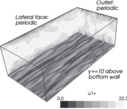
is used as a reference. An illustration of this test-case is given in Fig.1. The mean-ﬂow is oriented along the x-direction and plane walls bound the ﬂow at y = 6d. Periodicity is imposed in the streamwise and spanwise directions. The computa-tional domain extends over Lx3 Ly3 Lz= 2pd3 2d3pd ssame as the reference DNSd. The grid is Cartesian with 493 893 41 points; a tanh distribution is used in the y-direction. In the turbulent regime, the grid spacing is Dx+

= 52sin wall unitsd, Dy+

= 0.5 at the walls11 points be-low y+= 10d, and Dy+

= 24 at centerline, Dz+= 31. This mesh density respects standard recommendations for LES, as re-FIG. 1. Instantaneous contours of u1

+_{swall unit streamwise velocityd in the}

turbulent regime, obtained from the computation using the SISM-ES. As expected, the turbulent ﬂow develops streaky structures in the near-wall region.

(8)

viewed, for example, in Ref.2. Besides, a very small nondi-mensional time step, Dt+= Dtuw/_d_{= 3 3 10}−5_{, is imposed by} the explicit discretization. The pressure is reduced to obtain a Mach number Ma. 0.2 at the centerline, in order to optimize the convergence of the compressible solver, while keeping incompressible ﬂow conditionsstypically, throughout the do-main at the last instant, density lies within 1% of the initial densityr= 1.214 kg m−3d. The momentum in the x-direction is maintained by a uniform sover the whole ﬂowd source term that is adjusted dynamically to match the objective mean centerline velocity scalculated as the product of the DNS nondimensional mean centerline velocity and uw = 0.59 m s−1_{d on the one hand. The friction velocity is a}

result of the simulation on the other hand. Actually, for a turbulent velocity profile, the calibration of the mean center-line velocity allows a rather effective calibration of the vol-ume flow ratesor the mass flow rate, given the incompress-ibility of the flowd. This is checked numerically by integrating the mean axial velocity profile with the Simpson rule for nonregular grids. The volume flow rate difference between the different LES simulations and the reference DNS sdimensionalized at the present flow conditionsd is lower than 1%. This calibration is consistent with common practice in real flows, where the incident velocity or the volume/mass flow rate is fixed. Moreover, the fixed center-line velocity is a stringent condition when evaluating the description of the wall region.

The numerical results are nondimensionalized with the channel half width,d, and the objective friction velocity, uw. The use of the objective friction velocitysinstead of the com-puted friction velocityd as reference velocity is rather un-usual, and will be discussed when addressing the mean ve-locity proﬁle.

Four LESs have been carried out with different subgrid-scale models:

• The shear-improved Smagorinsky’s model with a spa-tial average over the x and z directionssSISM-SAd. • The shear-improved Smagorinsky’s model with an

ex-ponential smoothingsSISM-ESd. The smoothing factor cexp is constant over the whole domain. The

cutoff frequency is ﬁxed at fc= uw/d, which yields cexp= 1.073 10−4 from Eq. s9d. This cutoff frequency

is expected to be representative of the largest eddies and provide a reasonable estimate of the lower bound of the turbulent spectrum.

• The shear-improved Smagorinsky’s model with an adaptive Kalman ﬁltering sSISM-AKFd. In a consis-tent way with the exponential smoothing,

sdfug=

2pfcDt

Î

3 u

p

,

with the characteristic velocity up= uw and the cutoff frequency fc= uw/_d_{; uw} _{is the objective friction} velocity.

• The ﬁltered-structure-function model sFSFd.30

The most general FSF formulation sknown as the six-neighbor formulationd is used. There is no preferred direction in the discretization stencil.

2. Instantaneous velocity probes and smoothing methods

The different smoothing strategies used for the SISM are illustrated on the velocity signal recorded by a probe at y+= 10sx = 0.19Lxand z = 0.23Lzd. The instantaneous velocity component, u1

+

, is displayed in Fig.2, together with the mean estimate,fu1

+

g, resulting from the three different smoothings. The transition to turbulence, characterized by the develop-ment of turbulent fluctuations and the increase of the mean velocity, is observed for 6 # t+# 12. The high frequencies are obviously suppressed from the smoothed signals. Neverthe-less, some low-frequencies persist for the exponential smoothing and the adaptive Kalman filtering as expected from their low-pass behavior. The spatial averagefFig.2sadg removes nearly all the fluctuations in the turbulent regime and captures the evolution of the mean velocity from the laminar to the turbulent regime. This average is very efficient indeed, however, it requires spatial homogeneity; a condition which is hardly met in complex flow configurations.

Concerning the exponential smoothing fFig. 2sbdg, the cutoff period was ﬁxed at Tc

+

= 1. Velocity ﬂuctuations with a period exceeding Tc

+

are maintained. Besides, the character-istic time related to the streamwise advection sthrough the whole channeld may be estimated as Dtconv

+

= Lx

+_/_ku 1 +_{l . 0.82}

at y+= 10. The exponential smoothing therefore retains dy-namical ﬂuid structures whose period is larger than Dtconv

+

. Such events are actually trapped between the periodic streamwise boundary conditions, passing several times in circles through the channel. This feature enforces artificial temporal correlation and weakens the smoothing. This streamwise periodicity is an artifact of the channel-flow con-figuration that should not occur in practical concon-figurations; the exponential smoothing should then be more regular. For comparison, the spatial average in the x-direction is cal-culated a posteriori. Interestingly, the x-average follows quite accuratelyswith a short time leadd the variations of the

0 4 8 12 16 u₁+ 0 4 8 12 16 u₁+ 0 5 10 15 20 25 t+ 0 4 8 12 16 u₁+ (a) (b) (c) +4

FIG. 2. Numerical velocity probes at y+_{= 10}_{sx = 0.193 L}

xand z = 0.233 Lzd for the simulations with spatial average: SISM-SAsad, exponential smooth-ing: SISM-ES sbd, and adaptive Kalman ﬁltering: SISM-AKF scd. Dots: instantaneous velocity u1

+_{; continuous lines: estimated mean velocity} _fu 1 +_g.

The dashed-line in sbd is the postprocessed spatial average along the

(9)

exponential smoothing. This may be explained by the fact that roughly speaking, the whole velocity proﬁlesalong the x-directiond passes through the probe during a time interval Dtconv

+

of the order of the “memory time,” Tc

+

. Therefore, the exponential smoothing sin timed is mainly equivalent to the spatial average in the streamwise direction. However, this former does not require any homogeneity conditions. It is local in space and time while the x-average relies on a 48-point stencil. Finally, the adaptive Kalman ﬁltering fFig. 2scdg behaves qualitatively in a similar way as the exponen-tial smoothing but with a cutoff frequency that adapts itself locally. Here, at y+= 10, this appears to give smoother results. This feature will be investigated next.

3. Velocity profiles and energy spectra

The mean velocity proﬁle and the turbulent intensity proﬁles sin the stabilized turbulent regimed are displayed in Fig. 3 and compared with DNS data. In the post-processing, the averagesdenoted by kld is meant over space sx and z directions, y-mirrord and time s111 samples for 11.8# t+_{# 28.0d.}

In the present paper, the reference velocity for scaling is the objective friction velocity suw= 0.59 m s−1_{d. The main}

graph of Fig.3sadis plotted with this convention. However, a graph of the results plotted with a more conventional scaling sbased on the computed friction velocityd is inlaid in the major graph, for comparison with literature. The convention of the present paper is preferred because the uniﬁed scaling velocity allows a direct comparison between the different versions of LES. More importantly, it makes the nondimen-sional mean centerline velocity match the reference DNS, which is consistent with the strategy of calibration. In com-parison, the centerline error observed in the inlaid graph, using the more conventional scaling, actually comes from the friction velocity error sthe mean centerline velocity being imposedd. Finally, the present convention allows quantifying the velocity proﬁle quality by considering the friction veloc-ity value.

Considering the major graph of Fig. 3sad, a satisfactory prediction of the mean velocity proﬁle is achieved by the

different models. The FSF model yields the best prediction but the different SISM implementations are close, with little inﬂuence of the smoothing method. The objective friction velocity uw is 0.59 m s−1 _{sfrom the reference DNSd}

com-pared to 0.60 m s−1 _{for FSF, 0.53 m s}−1 _{for SISM-SA, and}

0.54 m s−1 _{for SISM-ES and SISM-AKF. In terms of the}

Reynolds number, these values for the friction velocity yield Rew= 402 for FSF, Rew= 355 for SISM-SA, and Rew= 362 for SISM-ES and SISM-KF, as opposed to Rew= 395 for the DNS. Even though the FSF model provides the best estimate, the different SISM implementations lie within 10% of the objective value, respecting the level of accuracy reviewed in Ref. 31 for standard SGS models. The turbulent intensity proﬁles are also well-captured for the three velocity compo-nents. Here, the SISM provides results closer to the DNS data than the FSF model. Little inﬂuence of the smoothing method is again observed.

The spanwise spectra of the streamwise velocity are shown in Fig. 4 for wall-normal distances y+= 10 and y+= 100. The LES spectra are in close agreement with the DNS in the range of energy-carrying wavenumbers and the dependence on y+_{is suitably captured. This ability to capture}

only the large-scale phenomena swith a moderate grid

den-1 10 100 y+ 0 5 10 15 20 <u₁+> DNS Moser et al.

LES SISM spatial average (SISM-SA) LES SISM exponential smoothing (SISM-ES) LES SISM adaptive Kalman filter (SISM-AKF) LES Filtered Structure Function (FSF)

1 10 100 0 5 10 15 20 (a) 0 100 200 300 400 y+ 0 0.5 1 1.5 2 2.5 3 u_i’+ DNS Moser et al.

(b) u 1’ + u₂’+ u 3’ +

FIG. 3. Mean streamwise velocity proﬁlesad and turbulent intensity proﬁles sbd. The inlaid graph in sad presents the mean velocity results scaled by the computed friction velocitysinstead of the objective value used for the other plotsd.

10 100 κ.δ 1e-04 1e-03 1e-02 1e-01 1e+00 E_uu+ DNS Moser et al.

y+=10

y+=100

(10)

sityd makes the genuine interest, and difﬁculty as well, of large-eddy simulations. The SISM gives slightly better re-sults than the FSF modelswith little inﬂuence of the smooth-ing methodd.

4. Two-point velocity autocorrelations

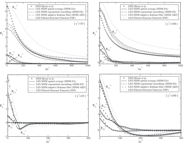
The two-point velocity autocorrelations in the stream-wise and spanstream-wise directions are displayed in Fig. 5 for y+_{= 10 and y}+_{= 100. Interestingly, our SISM implementations}

appear particularly effective in capturing the correct depen-dence on the separation distance. Again, the choice of the smoothing method has no noticeable effect. The major trends are fulﬁlled, that is to say,sid the correlations spread further in the direction of the ﬂow sx-directiond because of the streaky structures sevidenced in Fig. 1d and siid when y in-creases, correlations spreadsin x and z directionsd and aniso-tropy is reduced between the velocity components. In com-parison, the FSF model appears slightly less effective in capturing the DNS data. Finally, let us remark that the peri-odic boundary conditions and the domain extent do not allow for a proper decorrelation in the streamwise direction sLx

+

= 1241d, as evidenced by R11at y+= 100. This is a known

issue of this test ﬂow. The correlation timest_ii+

of the three components of the ﬂuctuating velocity, deﬁned by kui

8

stdui

8

st +tiidl / kui

8

2

l = 1 / 2 for i = 1 , 2 , 3, are plotted in Fig.6. Here only, the averagek · l is meant over space sz direction and y-mirrord and time

s3000 samples for 28.6# t+_{# 29.5d. Only the results for the}

exponential smoothing sSISM-ESd are reported. It is found that the correlation times globally decrease with the distance from the wall and thatt11sin the streamwise directiond

domi-nates overt22 andt33. The cutoff period of the exponential

smoothingsTc

+

= 1d and the mean cutoff period of the Kalman ﬁltersfrom SISM-AKFd are also displayed in the ﬁgure. This latter is obtained by identifying the optimal Kalman gain, K, with the smoothing factor of the exponential smoothing and by using Eq. s9d in order to relate this smoothing factor to

0 200 400 600 800 1000 ∆x + 0 1 2 3 4 5 6 7 R_ii+ DNS Moser et al.

[ y+=10 ] R₁₁+ R 22 + R 33 + 0 200 400 600 800 1000 ∆x + 0 1 2 3 R_ii+ DNS Moser et al.

[ y+=100 ] R₁₁+ R₂₂+ R₃₃+ 0 100 200 300 400 ∆z + -2 0 2 4 6 R_ii+ DNS Moser et al.

[ y+=10 ] R₁₁+ R 22 + R₃₃+ 0 100 200 300 400 ∆z + 0 1 2 3 R_ii+ DNS Moser et al.

[ y+=100 ] R₁₁+ R₂₂+ R 33 +

FIG. 5. Two-point velocity autocorrelations for streamwise separationssupd and spanwise separations sdownd at y+_{= 10}_{sleftd and y}+_{= 100}_srightd.

0 100 200 300 400 y+ 0.01 0.1 1 T+ τ 11 +

LES SISM exponential smoothing (SISM-ES) τ

22 +

LES SISM exponential smoothing (SISM-ES) τ

33 +

LES SISM exponential smoothing (SISM-ES) T_c+LES SISM exponential smoothing (SISM-ES) T_c+LES SISM adaptive Kalman filter (SISM-AKF)

FIG. 6. Correlation times of the three components of the ﬂuctuating velocity and cutoff periods, Tc

+_{, of the exponential smoothing and the adaptive}

(11)

Tc; 1 / fc. This ﬁnally yields Tc

+

= 2pDt+_/

Î

_{3kKl, where k · l is}

the usual postprocessing average. The two cutoff periods are found about 20 times larger than the correlation times of the velocity fluctuations, indicating that the two smoothing methods are indeed efficient at filtering out the turbulent fluctuations. The mean cutoff period of the adaptive Kalman filter remains close to 1 but decreases with the wall-normal distance, following the behavior of the velocity correlation times. This is very reasonable since the Kalman filter is ex-pected to adapt its cutoff period according to the observed velocity fluctuations. In this test flow the spatial variation of the correlation times is rather moderate, which explains that the mean cutoff period of the adaptive Kalman filter remains actually very close to the constant cutoff period of the expo-nential smoothing. This justifies why the two methods mostly behave the same way.

In summary, the results of our SISM-based LES of the channel flow are in good agreement with the reference DNS data for both one- and two-point statistics. The SISM, by explicitly accounting for the mean-flow through a rather simple formulation, reaches predictive qualities similar to the filtered-structure-function model on this test flow. Regarding the extraction of the mean-flow, the exponential smoothing and the adaptive Kalman filter appear to be particularly con-venientscomputationally sober, local in spaced and efficient methods, yielding results essentially similar to the spatial averagesin this simple-geometry flowd. A more severe test will be considered in the next section.

C. Flow past a cylinder in the subcritical turbulent regime

The numerical simulation of flows around bluff bodies is a great challenge for LES.32In this respect, the flow past a circular cylinder at high Reynolds numbers is of special importance.33 The shear-layer transition regime is a well-documented case that involves complex phenomena and, therefore, deserves interest for our purpose. Here, the defini-tion of the mean-flow requires attendefini-tion. The boundary layer separationsat the origin of the vortex sheddingd occurs up-stream the transition, which makes the vortex-shedding part of thesunsteadyd mean-flow. Moreover, contrary to the chan-nel flow, there is no homogeneous direction, not even span-wise, because of the three-dimensionality of the vortex shedding.34 Therefore, unsteady local smoothing strategies are necessary to extract the mean-flow. Two SISM computa-tions are presented, implementing the exponential smoothing sSISM-ESd and the adaptive Kalman filtering sSISM-AKFd, respectively.

1. Numerical simulation settings

A circular cylinder of axis z with diameter D = 2R = 0.01 m is set in an undisturbed airﬂow with velocity U`

= 70 m s−1 _{along the x-direction}_{sunder standard conditions}

of temperature and pressured. The diameter-based Reynolds number is ReD= 4.73 104, within the subcritical turbulent re-gime range smore precisely, the shear-layer transition re-gimed. This ﬂow is complex and experiences laminar bound-ary layer separation, shear-layer transition in the vicinity of the cylinder, turbulent wake, and von Kármán vortex shed-ding at the Strouhal number St= fsD / U_`< 0.2, yielding fs < 1400 Hz for the objective vortex-shedding frequency. FIG. 7. Cylinder mesh at constant z. Left: global view; right: close-up view

around the cylindersevery second point in each directiond.

FIG. 8. Mean velocity ﬁeld obtained from the SISM-ES computation. Up: contours of nondimensional streamwise velocitykUl / U`. Down: velocity

vectorskUWl. The gray square indicates the end of the recirculation bubble.

FIG. 9. Nondimensional vorticity fieldsz componentd from the SISM-ES computation. Left: instantaneous field; right: exponentially smoothed field at the same instant.

0.024 0.026 0.028 0.03 0.032 0.034 0.036 0.038 0.04 0.042 0.044 −1.5 −1 −0.5 0 0.5 1 1.5 t [s] C

FIG. 10. Temporal evolution of lift and drag coefﬁcients for the SISM-ES computation.s…d CL;s—d CD.

(12)

The aspect ratio of the cylindersspan length over radiusd has some inﬂuence on the ﬂow,35 which explains partly the dispersion of the experimental results at comparable Rey-nolds numbers. In our LES, the grid extends over 3D in the spanwise directionsz-directiond but periodicity is imposed on the end planes so that the computations can be representative of higher aspect ratios. Views of the grid are displayed in Fig.7. The computational domain extends over 10D in the radial direction and the whole grid uses 3 3 106points. In the turbulent region, behind the separation line, the wall grid densitysin wall unitsd is Drmax

+

. 1 swith a radial growth ratio of 1.2d, RDu_max+ . 20, and Dzmax

+

. 25. Again, this mesh den-sity respects standard recommendations for LES.2The non-dimensional time step is Dt+= DtU`/D= 4 3 10−4, adapted to

explicit discretization.

The SISM-ES computation relies on a ﬁxed smoothing factor cexp= 6.0933 10−4 sthroughout the whole domaind.

This value of cexp is obtained from Eq. s9d with fc= 2fs, where fs< 1400 Hz is the objective vortex-shedding fre-quency. The cutoff frequency is ﬁxed at twice the vortex-shedding frequencysthe factor 2 is arbitraryd in order to en-sure that the vortex shedding is suitably captured in the mean-ﬂow reconstruction. The SISM-AKF computation re-quires for calibration a reference velocity, up, and a reference frequency, fcfcf. Eqs.s11dands14dg. Our natural choices are up= U`and fc= fs. Contrary to the exponential smoothing, in

which fcrepresents the actual cutoff frequency, fc is here a reference value pointing out the order of magnitude of the cutoff frequency. This latter adapts itself to the local behav-ior of the ﬂow according to the Kalman ﬁltering procedure. Finally, the computations have been recorded over 24 peri-ods, representing nearly 3000 samples in the established tur-bulent regime.k · l denotes the postprocessing time and span-wise average.

2. Flow field, forces, and Strouhal number

An overview of the ﬂow resulting from the SISM-ES computation is presented at ﬁrst. The mean streamwise

ve-locity, kUl, is represented in the upper half of Fig. 8. The gray square dot delimits the recirculation bubble: the “wake-closure length” lc is given by kUlsx = lc, y = 0d = 0. In the lower half of the figure, the mean velocity vector fieldkUWl is displayed. The mean recirculation zone can be clearly iden-tified. In Fig. 9, the z-components of vorticity for both the instantaneous flow and the exponentially smoothed flow are compared at the same instant. While the instantaneous vor-ticity exhibits a wide range of structure sizes, the exponential-smoothed flow mostly captures the vortex shed-dingswhere shear effects are significantd, as expected. Figure 10displays the temporal evolution of the lift coefficient, CL, and drag coefficient, CD, over 24 periods of vortex shedding. As already mentioned in Refs.36 and37, a strong correla-tion is observed between the variacorrela-tions of CDand the modu-lation of CL; typically, the value of the drag is high when the lift amplitude is maximum.

These ﬁrst qualitative results are very satisfactory. Here, only the results with exponential smoothing are shown, but very similar features have been observed for the SISM com-putation with the adaptive Kalman ﬁlter.

Quantitative comparisons are now carried out between the SISM-ES, the SISM-AKF, and available experimental datasat comparable Reynolds numbersd. The mean drag co-efﬁcient, kCDl, the root-mean-square drag coefﬁcient, CD

8

, and the root-mean-square lift coefﬁcient, C_L

8

, are gathered in TableI. While the two smoothing methods had yielded very similar results for the channel-ﬂow computations, notable differences are obtained here. However, both computations give forces that lie within the experimental ranges.

The vortex shedding has a strong impact on the pressure distribution around the cylinder and, therefore, on the lift and drag oscillations. Except from the rearmost part of the cylin-der, the wall pressure spectrum is peaked around the shed-ding frequency, fs. From the wall pressure spectrum at

u= 90° su is the angle taken from the upstream stagnation pointd, the vortex-shedding frequency has been identiﬁed: TABLE I. Force coefﬁcients and Strouhal number for the LES in comparison with experimental data.

SISM-ES SISM-AKF Data in literature kCDl: mean drag coefﬁcient 1.34 1.23 1.35sReD= 4.33 104d, Ref.35

f1.0, 1.35g sReD= 4.83 104d, Ref.38 f1.0, 1.3g sReD= 4.83 104d, Ref.39 f1.1, 1.3g sReDPf104, 105gd, Ref.37

CD8: rms drag coefﬁcient 0.09 0.065 0.16sReD= 4.33 104d, Ref.35 f0.08, 0.1g sReD= 4.83 104d, Ref.40 f0.05, 0.1g sReDPf104, 105gd, Ref.37

CL8: rms lift coefﬁcient 0.77 0.603 f0.45, 0.55g sReD= 4.33 104d, Ref.35 f0.4, 0.8g sReD= 4.83 104d, Ref.40 f0.6, 0.82g sReDPf104, 105gd, Ref.37 St: Strouhal number 0.190 0.204 f0.18, 0.2g sReD= 4.83 104d, Ref.38

(13)

• SISM-ES computation: fs= 1330 Hz corresponding to a Strouhal number St= 0.190;

• SISM-AKF computation: fs= 1422 Hz corresponding to St= 0.204.

In Table I, this key criterion is shown to be in very good agreement with the available experimental data.

3. Wall friction and pressure distribution

Figure 11 shows the distribution of the mean friction coefﬁcient, kCfl ;

f

ktwl /1

2rU` 2

_g

Î

ReD swhere tw is the fric-tiond, around the cylinder. Both computations are in good agreement with the experimental data, with however a slightly better matching for the SISM-AKF. The mean sepa-ration angle, u_s, is the angle for whichkCfl vanishes. Here, the measured values areus= 88° for the SISM-ES computa-tion and us= 86° for the SISM-AKF computation swith an angular resolution of Du= 2° in this regiond. According to experimental data37in the range 4.03 104_{# Re}

D# 4.53 104, the expected separation angle isus< 83°. The LES compu-tations appear to slightly overestimateusbut the discrepancy is only two grid points.

In the channel-ﬂow simulation, the cutoff frequency for the exponential smoothing had been evaluated by fc= uw/_d_, withdbeing the half widthsreference length of the ﬂowd and uwthe friction velocitysreference velocity based on the shear at the walld. Along the same line of idea, a cutoff frequency may be designed here from the radius of the cylinder sR = D / 2d and the maximal value of the skin friction velocity on the cylinder, that is,

fshear=

maxsuwd

R . s17d

Numerically, this yields fshear= 1430 Hz in the SISM-ES

computation. This frequency is expected to be representative of the largest turbulent eddies detaching from the cylinder. Interestingly, this is almost equal to the vortex-shedding fre-quency sfs< 1400 Hzd characterizing the mean-flow un-steadiness. The proximity between the frequency associated with the flow unsteadinesssfsd and the frequency of the larg-est turbulent eddies sfsheard indicates that the mean-flow

re-construction using time-domain filtering necessarily includes sto some extentd the dynamics of large-sized energy-carrying turbulent eddies. One may evaluate that our mean-flow re-construction encompasses turbulent velocity fluctuations within the frequency band fshear, f , fc< 2fshear ssince f_s< fsheard. This is an unavoidable limitation of our method

salready mentioned in Sec. IId. However, the present results show that this limitation does not seem to dramatically im-pact on the quality of the whole modeling. A similar reason-ing can be followed for the adaptive Kalman ﬁlterreason-ing. In that case, the cutoff frequency remains of the order of fshear and

adapts itself dynamically to the ﬂuctuations of the ﬂow. This strategy appears to yield better results.

The distribution of the mean pressure-coefﬁcient, kCpl ; skpl − p`d /

1 2rU`

2

, around the cylinder is shown in Fig. 12 and compared with various experimental data. The prediction is very satisfactory for both SISM computations.

Finally, the distribution of the root-mean-square pressure-coefﬁcient, Cp

8

, is plotted in Fig. 13. The overall behavior is well-captured with a maximum around the point of separation.42The intensity is notably overestimatedsabout 50% on the peak leveld by the SISM computation with ex-ponential smoothing but the computation with the adaptive Kalman ﬁltering captures much more accurately the experi-mental levels sparticularly those closer to the simulated ReD= 4.73 104d. This is another illustration of the inﬂuence of the smoothing approach on this test-case.

4. Wake-centerline mean velocity

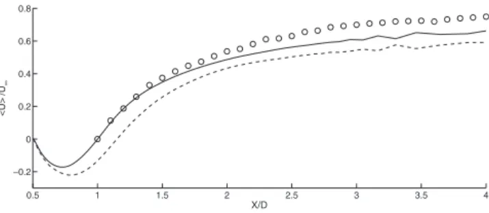
Figure14displays the mean velocitykUl along the wake centerline for both SISM computations, in comparison with the experimental results reported in Ref. 38 at ReD= 1.4

0 50 100 150 200 250 300 350 −0.5 0 0.5 1 1.5 2 2.5 3 θ[deg.] <Cf>

FIG. 11. Circular cylinder skin friction coefﬁcient. s——d SISM-ES at ReD= 4.73 104; s– – –d SISM-AKF at ReD= 4.73 104; ssd experimental data sRef. 42d at ReD= 9.13 104; shd experimental data sRef. 39d at ReD= 105. 0 20 40 60 80 100 120 140 160 180 −2 −1.5 −1 −0.5 0 0.5 1 θ[deg.] <Cp>

FIG. 12. Mean pressure-coefﬁcient distribution,kCpl, around the cylinder. s——d SISM-ES at ReD= 4.73 104;s– – –d SISM-AKF at ReD= 4.73 104; snd experimental data sRef.35d at ReD= 4.03 104;ssd experimental data sRef.43d at ReD= 4.63 104;shd experimental data sRef.39d at ReD= 105.

0 20 40 60 80 100 120 140 160 180 0 0.1 0.2 0.3 0.4 0.5 0.6 0.7 θ[deg.] Cp’

FIG. 13. Root-mean-square pressure-coefﬁcient, Cp8, around the cylinder. s——d SISM-ES at ReD= 4.73 104;s– – –d SISM-AKF at ReD= 4.73 104; shd experimental data sRef.41d at ReD= 6.13 104;snd experimental data sRef.36d at ReD= 6.13 104;ssd experimental data sRef.42d at ReD= 105; sLd experimental data sRef.44d at ReD= 105.

(14)

3 105_{. The behavior and levels are globally captured. A}

spe-ciﬁc attention can be drawn on the mean separation bubble length sor wake-closure lengthd, lc, given by kUlsx = lc, y = 0d = 0. In this regime, lcis expected to lower with increas-ing Reynolds number.45 For the present LES with ReD= 4.7 3 104

, it should to be close to lc. 1.25D. The SISM-ES computation yields lc= D, surprisingly close to the value of the experimental proﬁle at ReD= 1.43 105. A much better prediction is again achieved by the SISM-AKF with lc= 1.15D.

In summary, LES of the flow past a circular cylinder at ReD= 4.73 104 was carried out using the SISM with two different mean-flow extraction strategies: An exponential smoothingsa baseline methodd and an adaptive Kalman filter san elaborated methodd. A good overall prediction of this complex flow was achieved for both smoothing methods. However, when using the exponential smoothing some dis-crepancies have been observed on the mean friction, wall pressure fluctuations, and wake-centerline mean velocity. All these discrepancies are reduced by the use of the Kalman filter. This suggests the necessity of using adaptive snonhomogeneousd cutoff properties when treating complex snonhomogeneousd turbulent flows.

IV. SUMMARY AND CONCLUSION

The physical idea which underlies this study is to take into account the mean-flow inhomogeneities in the subgrid-scale viscosity. This feature is clearly encompassed in the shear-improved Smagorinsky’s model. Numerically, two dis-tinct smoothing algorithmssan exponentially weighted mov-ing average and an adaptive Kalman filterd are proposed to extract the mean-flow as the simulation progresses. Our re-sults indicate that the whole modeling offers an equitable compromise between the accuracy of the numerical solution and the computational cost. Since our method exploits the temporal discretization recurrently, it is entirely local in space and, therefore, suitable for parallelization and conve-nient for boundary conditions.

In the classical channel-flow test-case, this approach was shown to give satisfactory results regarding both mean and fluctuating velocities, spectra, and two-point correlations. Predictive capabilities appear comparable to the well-known filtered-structure-function model, used as reference. Further improvement of the present approach is still possible, as re-vealed by the channel configuration through the

underpredic-tion of fricunderpredic-tion velocity. Since the different smoothing strat-egies, i.e., the reference spatial average and the presently introduced temporal digital filters, appear to achieve very similar results, we believe that major benefit would rather be gained from the improvement of the snumericald discretiza-tion scheme and the subgrid-scale modeling sthe shear-improved Smagorinsky’s modeld. The subcritical turbulent flow past a cylinder has provided a more selective case for the smoothing methods, combining both nonhomogeneity and mean-flow unsteadiness. Extensive comparisons have been carried out with experimental datasat comparable Rey-nolds numbersd, concerning the global fluid forces acting on the cylinder, the vortex-shedding frequency, the mean skin friction, the mean and fluctuating pressure distribution saround the cylinderd, and the mean wake-centerline velocity. The numerical results using the exponential smoothing ex-hibit some discrepanciesswith experimental datad that are all reduced by using the adaptive Kalman filter. This latter yields a very satisfactory description of the flow characteris-tics. The adaptivity and efficiency of this modeling sshear-improved Smagorinsky’s model in combination with the adaptive Kalman filterd make it very relevant for LES of complex turbulent flows. Especially, applications to proper turbomachine flows are of actual interest.

In the Kalman filtering framework, introducing correla-tions in timesin order to better smooth the turbulent fluctua-tionsd is readily possible. However, this would significantly increase the computational cost and memory requirementssif several time steps need to be storedd. For that reason, this aspect was left out in the present work. Nevertheless, a pos-sible improvement may consist in treating the temporal smoothing from a Lagrangian viewpoint salong fluid trajec-toriesd. This is under investigation. Finally, the smoothing approaches investigated in the present work do not a priori require a grid-convergence analysis because they are purely temporal. However, since filtering acts on nonlinear turbulent quantities, which are definitively dependent on the spatial mesh resolution, a parametric study sas a function of the mesh resolutiond would certainly deserve interest as well.

ACKNOWLEDGMENTS

The authors would like to thank J.-P. Bertoglio, P. Flan-drin, L. Shao, and F. Toschi for long-term valuable discus-sions. The numerical simulations rely on the TURB’FLOW

solver, originating from the LMFA at the Ecole Centrale de Lyon and codeveloped with the FLUOREM company sFranced. Simulations have been performed by using the lo-cal computing facilities at LMFA and ENS-Lyon sPSMNd, and national HPC resources of CINESsMontpellier, Franced.

1

M. Lesieur, O. Métais, and P. Comte, Large-Eddy Simulations of

Turbu-lencesCambridge University Press, Cambridge, 2005d.

2

P. Sagaut, Large Eddy Simulation for Incompressible Flows: An

Introduc-tion, 3rd ed.sSpringer-Verlag, Berlin, 2006d.

3

U. Piomelli, “Large-eddy simulation: Achievements and challenges,”

Prog. Aerosp. Sci. 35, 335s1999d.

4

This argument holds if neglecting noncommutation errors between the ﬁlter and partial derivatives.

5

S. B. Pope, Turbulent Flows sCambridge University Press, New York, 2000d.

6

C. Meneveau and J. Katz, “Scale-invariance and turbulence models for

0.5 1 1.5 2 2.5 3 3.5 4 −0.2 0 0.2 0.4 0.6 0.8 X/D <U> /U∞

FIG. 14. Mean velocitykUl along the wake centerline. s——d SISM-ES at ReD= 4.73 104; s– – –d SISM-AKF at ReD= 4.73 104; ssd experimental datasRef.38d at Re= 1.43 105_.