HAL Id: tel-00917657
https://tel.archives-ouvertes.fr/tel-00917657
Submitted on 12 Dec 2013HAL is a multi-disciplinary open access archive for the deposit and dissemination of sci-entific research documents, whether they are pub-lished or not. The documents may come from teaching and research institutions in France or abroad, or from public or private research centers.
L’archive ouverte pluridisciplinaire HAL, est destinée au dépôt et à la diffusion de documents scientifiques de niveau recherche, publiés ou non, émanant des établissements d’enseignement et de recherche français ou étrangers, des laboratoires publics ou privés.
Alexandru Berbecea
To cite this version:
Alexandru Berbecea. Multi-level approaches for optimal system design in railway applications. Other. Ecole Centrale de Lille, 2012. English. �NNT : 2012ECLI0024�. �tel-00917657�
N° d’ordre : 199
E
COLEC
ENTRALED
EL
ILLETHESE
présentée en vue d’obtenir le grade deDOCTEUR
en Spécialité : Génie Electrique parAlexandru BERBECEA
DOCTORAT DELIVRE PAR L’ECOLE CENTRALE DE LILLE
Titre de la thèse :Multi‐level approaches for optimal system design
in railway applications
Approches multi‐niveaux pour la conception systémique optimale des
chaînes de traction ferroviaire
Soutenue le 10 Octobre 2012 devant le jury d’examen :Examinateur L. Krähenbühl Directeur de recherche CNRS, Président du Jury
Ecole Centrale de Lyon
Rapporteur J.‐L. Coulomb Professeur INP Grenoble
Rapporteur B. Sareni Professeur ENSEEIH Toulouse
Examinateur S. Vivier Maître de conférences HDR UT de Compiègne
Examinateur S. Brisset Maître de conférences HDR Ecole Centrale de Lille
Directeur de thèse F. Gillon Maître de conférences HDR Ecole Centrale de Lille
Co‐directeur P. Brochet Professeur Ecole Centrale de Lille
Invité E. Batista Ingénieur Alstom Transport, Tarbes Thèse préparée dans le Laboratoire L2EP à l’Ecole Centrale de Lille
Multi‐level approaches for optimal system design
in railway applications
Alexandru Berbecea
October, 10th 2012Résumé
Dans le contexte actuel de mondialisation des marchés, le processus classique de conception par essais et erreurs, traditionnellement employé par les ingénieurs, nʹest plus capable de répondre aux exigences de plus en plus accrues en termes de délais très courts, réduction des coûts de production, etc. Lʹoutil dʹoptimisation propose une réponse à ces questions, en accompagnant les ingénieurs dans la tâche de conception optimale.
Lʹobjectif de cette thèse est centré sur la conception optimale des systèmes complexes. Deux approches dʹoptimisation sont abordées dans ce travail: lʹoptimisation par modèles de substitution et la conception optimale basée sur la décomposition des systèmes complexes.
Lʹutilisation de la conception assistée par ordinateur (CAO) est devenue une pratique régulière dans l’industrie. La démarche dʹoptimisation basée sur modèles de substitution est destinée à répondre à lʹoptimisation des dispositifs avec ce genre de modèles coûteux de simulation, tels que les éléments finis (EF) en électromagnétisme. Lʹoptimisation multi‐objectif se présente comme un outil dʹaide à la décision, en aidant le concepteur à prendre une décision éclairée. Le calcul distribué est utilisé pour réduire le temps global du processus dʹoptimisation.
Les systèmes dʹingénierie tels que les chaînes de traction ferroviaires sont trop complexes pour être traités comme un tout. Les stratégies dʹoptimisation basées sur la décomposition cherchent à répondre à la conception optimale de ces systèmes. Les approches de décomposition par modèle, discipline ou objet visent à distribuer la charge de calcul. Des stratégies de coordination multi‐ niveaux sont utilisées pour gérer le processus dʹoptimisation. Ces approches permettent à chaque équipe de spécialistes de travailler sur leur expertise de façon autonome. Les techniques dʹoptimisation à base de modèles de substitution peuvent être intégrées dans les stratégies d’optimisation multi‐niveaux, allégeant ainsi la charge de calcul.
Les approches dʹoptimisation développées au sein de ce travail sont appliquées pour résoudre plusieurs problèmes dʹoptimisation électromagnétiques, ainsi que la conception optimale d’un système de traction ferroviaire de la Société Alstom.
Mots‐clés
Conception optimale des systèmes électromagnétiques Optimisation par modèles de substitution Conception optimale de systèmes complexes basée sur décomposition Optimisation multi‐niveaux Chaîne de traction ferroviaireAbstract
Within a globalized market context, the classical trial‐and‐error design process traditionally employed by engineers is no longer capable of answering to the ever‐growing demands in terms of short deadlines, reduced production costs, etc. The optimization tool presents itself as an answer to these issues, accompanying the engineers in the optimal design task.
The focus of this thesis is centered on the optimal design of complex systems. Two main optimization approaches are addressed in this work: the metamodel‐based design optimization and the decomposition‐based complex systems optimal design.
The use of computer‐aided design/engineering (CAD/CAE) software has become a regular practice in the engineering design process. The metamodel‐based optimization approach is intended to address the optimization of devices represented by such computational expensive simulation models, as the finite element analysis (FEA) in electromagnetics. The multi‐objective optimization stands as a decision‐making support tool, helping the design engineer make an informed decision. The distributed computation is employed to reduce the overall time of the optimization process.
Engineering systems such as railway traction systems are too complex to be addressed as a whole. The decomposition‐based optimization strategies are intended to address the optimal design of such systems. Model, discipline or object‐based decomposition approaches intend to distribute the computational burden across the system. Multi‐level coordination strategies are used to manage the optimization process. Each team of specialists can work independently at the object of their expertise. The metamodel‐based optimization techniques can be integrated within the multi‐level decomposition‐based strategies, reducing the computational burden.
The optimization approaches developed within this work are applied for solving several electromagnetic optimization problems and a railway traction system optimal design problem of the Alstom Company.
Keywords
Optimal design of electromagnetic devices Metamodel‐based optimization Decomposition‐based complex systems optimal design Multi‐level optimization Railway traction systemRemerciements
Ce travail a été réalisé dans le cadre dʹun projet de recherche – « OPtimisation de SIMulations » (OPSIM), au sein du « Laboratoire d’Electrotechnique et d’Electronique de Puissance de Lille » (L2EP) de l’Ecole Centrale de Lille, en collaboration avec la société Alstom Transport.
Je suis très reconnaissant à mon directeur de thèse, Dr. Frédéric GILLON, Maître de conférences HDR. Ses conseils et ses encouragements constants mʹont aidé à surmonter les périodes les plus difficiles dans la réalisation du travail de cette thèse.
Je tiens à remercier à Professeur Pascal BROCHET, mon co‐directeur de thèse et directeur de l’équipe « Optimisation » du L2EP pour le très bon accueil dans son équipe avec une ambiance chaleureuse.
Ce travail nʹaurait pas pu être achevé sans la contribution des autres membres de l’équipe du projet, Dr. Stéphane BRISSET, Maître de conférences HDR et Martin CANTEGREL, mon collègue dans le projet.
Je voudrais remercier à Professeur Jean‐Louis COULOMB, Professeur Bruno SARENI, Dr. Laurent KRÄHENBÜHL, Directeur de recherche CNRS et Dr. Stéphane VIVIER, Maître de conférences HDR pour leur disponibilité et le temps précieux qu’ils m’ont accordé en tant que membres de mon jury de thèse.
Je tiens à exprimer ma reconnaissance à Mr. Laurent NICOD, Manageur activités R&D chez Alstom Transport. Je remercie également à Mr. Marc DEBRUYNE, Mr. Philippe CARRERE et Mr. Emmanuel BATISTA, ingénieurs Alstom Transport pour leurs conseils et remarques précieuses. Je tiens à remercier également tous les professeurs et les membres du personnel du laboratoire, je pense en particulier à Professeur Michel HECQUET, Xavier MARGUERON, Xavier CIMETIERE et Simon THOMY pour leur support. Un grand merci à tous mes collègues du laboratoire, en particulier à Martin CANTEGREL, Jinlin GONG, Nicolas BRACIKOWSKI, Mathieu ROSSI, Ramzi BEN‐AYED, Sophie FERNANDEZ, Adrian POP, Pierre CAILLARD, Aymen AMMAR, Dan ILEA, Dmitry SAMARKANOV, Pierre RAULT, Wenhua TAN, Nicolas ALLALI, Matthias FACKAM, Sangkla KREUAWAN, Amir AHMIDI et François GRUSON. Je garderai en mémoire un très beau souvenir du temps passé avec vous à l’Ecole Centrale.
En fin, je suis fortement reconnaissant à ma grand‐mère, mes parents et ma copine pour leur soutien et leurs constants encouragements tout au long de ces années de thèse. Ils ont toujours été là pour moi et sans eux, tout cela n’aurait été possible.
Contents
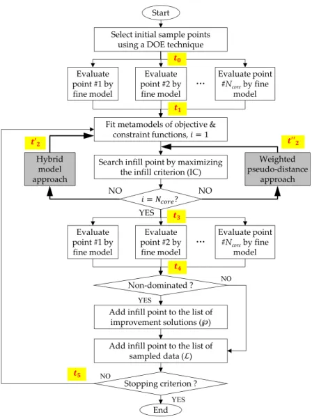
Introduction ... 25 Chapter 1 Decision support tools for complex electromagnetic systems design ... 29 1.1 General aspects of an optimal design process ... 29 1.2 Variables influence and correlation ... 31 1.3 Single and multi‐criteria optimization ... 34 1.3.1 Single‐objective optimization ... 34 1.3.2 Local vs. global optimality ... 35 1.3.3 Deterministic optimization algorithms ... 36 1.3.4 Stochastic optimization algorithms ... 37 1.3.5 Multiple criteria optimization ... 38 1.3.5.1 Pareto optimality ... 38 1.3.5.2 Decision making in the optimal design process ... 40 1.3.6 Optimization problem transformation techniques ... 41 1.3.6.1 Weighted objectives method ... 41 1.3.6.2 ‐constraint method ... 44 1.3.6.3 Goal‐attainment method ... 45 1.3.6.4 Other transformation techniques ... 47 1.3.6.5 Example test‐problem ... 47 1.3.7 Complex systems specific optimization strategies ... 50 1.3.7.1 Metamodel‐based optimization strategies ... 51 1.3.7.2 Decomposition‐based optimization strategies ... 51 1.4 Pareto front quality assessment tools ... 52 1.4.1 Metrics definition ... 53 1.4.2 Multi‐dimensional data representation ... 54 1.5 Commercial optimization software ... 55 1.6 Conclusion ... 562.1 Why optimizing using a metamodel? ... 57 2.2 Metamodel‐Based Design Optimization strategies ... 59 2.3 Sequential metamodel‐based optimization ... 61 2.4 Adaptive metamodel‐based optimization ... 64 2.4.1 General process ... 65 2.4.2 Multiple criteria ... 66 2.4.3 Well‐spread sub‐set selection from a metamodel‐optimal n‐dimension Pareto front .... 68 2.4.4 Application: LIM device design optimization problem ... 74 2.4.4.1 Modeling of the LIM device ... 74 2.4.4.2 Optimization problem formulation ... 76 2.4.4.3 Optimization results ... 76 2.5 Criterion‐based metamodel optimization ... 79 2.5.1 Single‐objective infill point selection criteria ... 79 2.5.2 Adaptive infill strategies ... 84 2.5.3 Constraint handling ... 86 2.5.4 Application: single‐objective SMES device optimization ... 91 2.5.5 EGO algorithm with multiple objectives (MEGO algorithm) ... 91 2.5.5.1 Existing multi‐objective extensions of the EGO algorithm ... 91 2.5.5.2 Pseudo‐distance infill point selection criterion ... 96 2.5.6 Multi‐objective EGO algorithm (MEGO) ... 98 2.5.7 Distributed computation‐suited MEGO ... 99 2.5.7.1 Hybrid model approach ... 100 2.5.7.2 Weighted pseudo‐distance approach ... 101 2.5.8 Development of the MEGO tool – graphical user interface ... 104 2.5.9 MEGO coupling with ModeFrontier® optimization software ... 105 2.6 Application: SMES device optimization problem ... 107 2.6.1 TEAM22 benchmark description ... 107 2.6.2 Modeling of the SMES device ... 109 2.6.3 Single‐objective optimization of the 3‐parameter TEAM22 benchmark problem ... 111 2.6.3.1 Optimal SMES design using classical global optimization strategies ... 111 2.6.3.2 Sequential metamodel‐based optimization of the SMES ... 113
2.6.3.3 Adaptive metamodel‐based optimization of the SMES ... 114 2.6.3.4 Criterion‐based metamodel optimization of the SMES (EGO algorithm) ... 115 2.6.4 Bi‐objective optimization of the SMES device ... 117 2.6.4.1 Bi‐objective SMES device optimization using MBDO ... 118 2.6.4.2 SMES optimization using the multi‐objective MEGO algorithm ... 118 2.6.4.3 SMES optimization using MEGO and the distributed computation ... 119 2.7 Conclusion ... 121 Chapter 3 Decomposition‐based complex system design optimization ... 123 3.1 Why need to decompose a complex system? ... 124 3.2 Complex system partitioning ... 125 3.2.1 Single‐level optimization strategies ... 126 3.2.2 Multi‐level optimization strategies ... 127 3.2.2.1 Model‐based complex system decomposition ... 128 3.2.2.2 Discipline‐based complex system decomposition ... 129 3.2.2.3 Object‐based (physical) complex system decomposition ... 130 3.3 Output Space Mapping (OSM) multi‐model optimization strategy ... 132 3.4 Collaborative Optimization (CO) multi‐discipline optimization strategy ... 136 3.4.1 Basic mathematical formulation of CO ... 137 3.4.2 Coordination of the CO process ... 138 3.4.3 Existing efficiency enhancements of the CO formulation ... 138 3.4.4 Efficiency enhancement of the CO process by integration of the Output Space Mapping (OSM) technique ... 140 3.5 Analytical Target Cascading (ATC) multi‐component optimization strategy ... 142 3.5.1 Basic mathematical formulation ... 143 3.5.2 All‐in‐One (AIO) optimization problem formulation ... 144 3.5.3 Coordination strategies for ATC decomposed systems... 146 3.5.4 Consistency constraints handling ... 149 3.5.5 Relaxation of the consistency constraints of the AIO problem ... 151 3.5.6 Penalty functions for the consistency constraint relaxation ... 152 3.5.6.1 Quadratic penalty relaxation ... 153 3.5.6.2 Lagrangian relaxation ... 154
multipliers ... 157 3.5.7 Mathematical example ... 158 3.5.8 Existing efficiency enhancements of the ATC process ... 166 3.5.9 Metamodel approximation integrated to the ATC formulation ... 167 3.6 Multi‐level optimization framework ... 169 3.7 Application: Optimal design of a low‐voltage single‐phase safety‐isolation transformer171 3.7.1 Transformer optimization benchmark ... 171 3.7.2 Transformer representation ... 172 3.7.3 OSM – MEGO isolation transformer optimization comparison ... 173 3.7.3.1 Single‐objective transformer optimization ... 174 3.7.3.2 Bi‐objective transformer optimization ... 177 3.7.4 Multi‐disciplinary optimization of the transformer by CO ... 179 3.8 Application: Optimal design of ultra‐capacitor energy storage system (UC‐ESS) on‐board a tramway ... 183 3.8.1 The ultra‐capacitor energy storage system (UC‐ESS) ... 183 3.8.2 Tramway traction system description ... 185 3.8.3 UC‐ESS multi‐level optimal design problem formulation ... 189 3.8.4 ATC formulation with adaptive‐metamodel approximation ... 191 3.9 Conclusion ... 195 Conclusion ... 199 Appendix A ... 203 Bibliography ... 207 Résumé étendu en français ... 219
List of Figures
Figure 1.1 : Correlation matrix ... 33 Figure 1.2 : Local vs. global optimality representation ... 35 Figure 1.3 : Pareto front representation for a generic bi‐objective optimization problem ... 39 Figure 1.4 : Weak Pareto solutions of the bi‐objective generic optimization problem ... 40 Figure 1.5 : Weighted objectives method applied to a bi‐objective optimization problem ... 42 Figure 1.6 : Weighted objectives method with improved non‐linear scalarization functions ... 44Figure 1.7 : ‐constraint method application for determining a design on the Pareto front of a bi‐ objective optimization problem ... 45
Figure 1.8 : Goal‐attainment method exemplification on a bi‐objective case ... 46
Figure 1.9 : Result of the 80*80 design grid evaluation for the analytical test‐problem ... 48
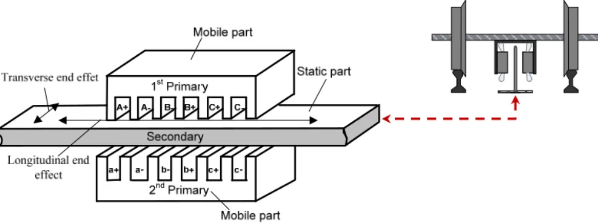
Figure 1.10 : Optimal results of the analytical test‐problem optimization employing the presented transformation techniques ... 49 Figure 2.1 : Different MBDO strategies ... 59 Figure 2.2 : Workflow of the sequential metamodel‐based optimization ... 62 Figure 2.3 : The modified Branin‐Hoo function ... 63 Figure 2.4 : Model comparison for the Branin‐Hoo modified function ... 63 Figure 2.5 : Adaptive metamodel‐based optimization process workflow ... 65 Figure 2.6 : Workflow of the multi‐objective adaptive MBDO technique ... 67 Figure 2.7 : Optimal solution of the Binh test problem ... 68 Figure 2.8 : Infill set selection for the Binh optimization test problem ... 69 Figure 2.9 : Pareto front of the Viennet optimization test problem ... 70 Figure 2.10 : Euclidian distance in the objective space between two points, 2 and 3 ... 71 Figure 2.11 : Summary of the selection point strategies ... 73 Figure 2.12 : Double‐sided linear induction motor (LIM) device ... 74 Figure 2.13 : The coupling between the electromagnetic (EMM) and thermal (TH) models ... 75 Figure 2.14 : Geometrical variables of the optimization problem ... 76 Figure 2.15 : Infill set selection of 10 well‐spread designs for evaluation using the FE model at the 1st MBDO iteration of the LIM device optimization ... 77 Figure 2.16 : Pareto front of the LIM device optimization using MBDO ... 77 Figure 2.17 : LIM optimization time decomposition ... 78
Figure 2.18 : Basic infill criteria, MinPred (exploitation) and MaxVar (exploration) for the modified Branin‐Hoo function ... 80
Figure 2.19 : Normal probability density and normal cumulative distribution functions ... 82
Figure 2.23 : Partitioning of the PI in n=5 levels of improvement ... 93
Figure 2.24 : Example of optimization using the pseudo‐distance infill criterion ... 98
Figure 2.25 : Multi‐objective Efficient Global Optimization (MEGO) algorithm flowchart ... 99
Figure 2.26 : Workflow for generating infill points using the “hybrid model” approach ... 100
Figure 2.27 : Workflow for generating points using the “weighted pseudo‐distance” approach ... 102
Figure 2.28 : MEGO algorithm workflow implementing the two strategies for distributing the calculi over several cores of one or more machines ... 103 Figure 2.29 : Main window of the MEGO graphical user interface (GUI) ... 104 Figure 2.30 : MEGO optimizer integration within ModeFrontier® environment ... 106 Figure 2.31 : 3D representation of the SMES device ... 107 Figure 2.32 : Representation of the right‐half transverse cut over the SMES device ... 108 Figure 2.33 : Critical curve for ensuring the superconductivity state of the superconductor ... 109 Figure 2.34 : General view over the FEM of the SMES device for a given configuration ... 110 Figure 2.35 : Zoom over the area containing the two coils of the SMES device ... 110 Figure 2.36 : Histogram of the SQP algorithm with 30 runs ... 112 Figure 2.37 : Box‐plot representation of the metamodels error measure, log ... 114 Figure 2.38 : Parallel coordinates representation of EGO algorithm runs with tested infill criteria 116 Figure 2.39 : Pareto front of the 8‐parameter TEAM22 optimization benchmark ... 118 Figure 2.40 : Pareto front results with distributed computation on different server configurations 119 Figure 2.41 : Speedup for the initial DOE and iteration step of the MEGO algorithm in the case of the SMES device optimization ... 120 Figure 3.1 : Complex system decomposition ... 125 Figure 3.2 : Different models that can be used in model‐based decomposition ... 129 Figure 3.3 : Discipline‐based complex system decomposition ... 130 Figure 3.4 : Object‐based (physical) complex system decomposition ... 131 Figure 3.5 : Example of complex system hierarchically and non‐hierarchically decomposed ... 132 Figure 3.6 : Output Space Mapping (OSM) information flow ... 133 Figure 3.7 : OSM optimal results for the analytical test‐case ... 135 Figure 3.8 : Structure and information flow of the collaborative optimization (CO) strategy ... 136
Figure 3.9 : Bi‐level CO structure implementing the OSM technique for the optimization of the disciplinary models of the isolation transformer ... 141 Figure 3.10 : Decomposed structure with local and exchanged variables ... 145 Figure 3.11 : Decomposed structure with local and exchanged variables with their copies ... 146 Figure 3.12 : Nested and simple loop coordination methods ... 146 Figure 3.13 : No‐loop coordination methods ... 148 Figure 3.14 : Representation of the variables of a sub‐problem ... 150 Figure 3.15 : General problem information flow ... 152 Figure 3.16 : ATC formulation with the nested Lagrangian dual problems ... 155 Figure 3.17 : Multi‐level representation of the analytical test problem ... 159 Figure 3.18 : Design variables evolution history for ATC employing the AL‐AD method ... 162 Figure 3.19 : Objective function and linking variables history representation ... 163
Figure 3.20 : Design variables evolution history using ATC with the AL‐AD method ... 164
Figure 3.21 : Design consistency and ATC convergence measures representation ... 165
Figure 3.22 : Workflow of the element actions at a given iteration of the ATC process using the adaptive metamodel approximation technique ... 168 Figure 3.23 : The structure of the ATC multi‐level optimization framework ... 170 Figure 3.24 : Safety‐isolation transformer to be optimized ... 172 Figure 3.25 : Coupling between the electromagnetic and the thermal FE models of the transformer ... 173 Figure 3.26 : Transformer compromise solutions obtained by the MEGO algorithm ... 175 Figure 3.27 : 3D Pareto front of the transformer benchmark obtained by the MEGO algorithm ... 178 Figure 3.28 : Transformer Pareto front . 1 comparison of OSM and MEGO ... 179 Figure 3.29 : Multi‐disciplinary isolation transformer representation ... 180
Figure 3.30 : System and discipline‐level objective function evolution during the isolation transformer optimization process using CO ... 182 Figure 3.31 : Tramway with on‐board ultra‐capacitor energy storage system (UC‐ESS) ... 184 Figure 3.32 : Mission profile for the considered tramway ... 184 Figure 3.33 : Tramway with on‐board ultra‐capacitor energy storage system (UC‐ESS) ... 185 Figure 3.34 : Simplified energetic representation of the tramway embarking the UC‐ESS ... 186 Figure 3.35 : Ultra‐capacitor (UC) pack representation ... 186 Figure 3.36 : UC pack model description ... 187 Figure 3.37 : Chopper’s coil representation ... 187 Figure 3.38 : Chopper’s coil model description ... 187 Figure 3.39 : Heat sink representation ... 188 Figure 3.40 : Heat sink model description ... 188 Figure 3.41 : Tramway system model description ... 189 Figure 3.42 : System‐level targets/responses evolution ... 193 Figure 3.43 : Chopper’s coil targets/responses evolution ... 194
List of Tables
Table 2.1 : Global/local optima of the modified Branin‐Hoo function ... 63 Table 2.2 : True function/metamodel global optima comparison ... 64 Table 2.3 : Special cases of GEI ... 83 Table 2.4 : Role of the different modules in Figure 2.30 within the SMES optimization process ... 106 Table 2.5 : Design variables and constants for the three‐parameter TEAM22 benchmark ... 108 Table 2.6 : Design variables for the eight‐parameter TEAM22 benchmark ... 108 Table 2.7 : Optimal configuration of the SMES found by classical global optimization strategies .. 112 Table 2.8 : Optimal configurations of the SMES device’s outer coil obtained using the six runs of the sequential metamodel‐based optimization approach ... 113Table 2.9 : Optimal configurations of the SMES device’s outer coil obtained using the adaptive MBDO approach and the six metamodels ... 115
Table 2.10 : Optimal configurations of the SMES device’s outer coil obtained using the EGO algorithm with different infill point selection criteria ... 116
Table 2.11 : FEM evaluation time and speedup for the initial DOE phase (LHS of 80 points) ... 120
Table 2.12 : FEM evaluation time and speedup for the iteration phase of the MEGO algorithm ... 120
Table 3.1 : Optimal configuration of the analytical test problem ... 158
Table 3.2 : Multi‐level analytical test‐problem optimal results obtained by ATC with QP, for the attainable targets 1 , 2 2.84,3.10 ... 161 Table 3.3 : Multi‐level analytical test‐problem optimal results obtained by ATC with AL‐AD ... 162 Table 3.4 : Design consistency attainment for the analytical problem solved by ATC with AL‐AD 165 Table 3.5 : ATC process convergence attainment for the analytical problem ... 165 Table 3.6 : Comparison of OSM, MEGO and SQP optimal transformer results ... 176 Table 3.7 : Optimal results comparison of the CO multi‐level optimization process and SQP ... 182 Table 3.8 : Local design variables of the different optimization problems of the hierarchy... 192 Table 3.9 : Target variables optimal values obtained by ATC ... 192 Table 3.10 : Local constraints of the different optimization problems of the hierarchy ... 192
Symbols and notation
Abbreviations
AAO All‐At‐Once AIO All‐In‐One AL Augmented Lagrangian AL‐AD Augmented Lagrangian with the Alternating Direction method of multipliers ALC Augmented Lagrangian Coordination ANOVA Analysis of Variance ATC Analytical Target Cascading BLISS Bi‐Level Integrated System Synthesis CAD Computer‐Aided Design CAE Computer‐Aided Engineering CFD Computational Fluid Dynamics CO Collaborative Optimization CO‐OSM Collaborative Optimization with Output Space Mapping CSSO Collaborative Sub‐Space Optimization DOE Design of Experiments EGO Efficient Global Optimization EI Expected Improvement EMM Electromagnetic model EMM0 No‐load electromagnetic model ESS Energy Storage System EV Expected Violation FE Finite Element FEA Finite Element Analysis FEM Finite Element Model FPI Fixed Point Iteration GEI Generalized Expected Improvement GA Genetic Algorithm IDF Individual Disciplinary Feasible L linear penalty LHS Latin Hypercube Sampling LIM Linear Induction Motor LP Lagrangian relaxed problemMDO Multi‐Disciplinary Optimization MEGO Multi‐objective Efficient Global Optimization MOP Multi‐objective Optimization Problem Multi‐EGO Multi‐objective Efficient Global Optimization algorithm of Jeong and Obayashi NSGA‐II Non‐dominated Sorting Genetic Algorithm II OSM Output Space Mapping ParEGO Pareto Efficient Global Optimization PD Pseudo‐Distance criterion PF Probability of Feasibility criterion PI Probability of Improvement criterion PSO Particle Swarm Optimization Q quadratic penalty RBF Radial Basis Function RS Response Surface RSM Response Surface Methodology SM Space Mapping SMES Superconducting Magnetic Energy Storage device SOP Single‐objective Optimization Problem SQP Sequential Quadratic Programming STEEM Maximized Energy Efficiency Tramway System TEAM22 optimization benchmark problem of the SMES device TH thermal discipline THM thermal model UC Ultra‐Capacitor UC‐ESS Ultra‐Capacity Energy Storage System
Symbols
‖∙‖ square of the norm of a vector ∘ term‐by‐term multiplication of vectors scalar variable representing the step size for the update of the Lagrangian multipliers within ATC analysis model employed with the sub‐problem within the ATC structuremetamodel approximation of the analysis model employed with the sub‐problem within the ATC structure constant parameter for the update of coefficients within the AL relaxation of ATC ∁ the set of children of the sub‐problem within the ATC structure consistency constraint function vector of the sub‐problem within the ATC structure convergence measure at iteration k of the ATC optimization process dominance distance neighboring distance
, Euclidian distance between designs i and j in the objective space tolerance value tolerance value for the coupling variables of sub‐problem target matching in ATC tolerance value for the shared variables of sub‐problem target matching in ATC inconsistency tolerance vector representing the allowed level of inconsistency between the different disciplines within the CO formulation objective functions vector objective function objective function value computed using the coarse model objective function value computed using the fine model metamodel estimation of the objective function of the sub‐problem within the ATC structure k‐th objective function value of the i‐th objective function of the point from the current Pareto front, closest to the trial point value of the i‐th objective function of the j‐th point of the current Pareto front, which is dominated by the trial point minimum value of the objective function from a set of designs inequality constraint function value computed using the coarse model inequality constraint function value computed using the fine model i‐th inequality constraint function i‐th expensive inequality constraint function i‐th inexpensive inequality constraint function vector of inequality constraint functions equality constraint function value computed using the coarse model equality constraint function value computed using the fine model j‐th equality constraint function k‐th expensive equality constraint function k‐th inexpensive equality constraint function vector of equality constraint functions objective function of the i‐th disciplinary optimization ∗ optimal objective function of the i‐th disciplinary optimization list of evaluated designs list of support points for the metamodel construction at the sub‐problem at iteration k of the ATC optimization process Λ list of weighting coefficients vectors vector of weighting coefficients Φ normal cumulative distribution function normal probability density function ℘ Pareto front ℘ Pareto front found by the optimization algorithm ℘ true Pareto front penalty function for the relaxed AiO problem within the ATC formulation
augmented Lagrangian penalty function for the relaxed AiO problem within ATC Ψ objective function of the Lagrangian relaxed problem (LP) within ATC
Ψ′ objective function of the augmented Lagrangian relaxed problem (AL) within ATC Ψ∗ optimal objective function value of the Lagrangian relaxed problem (LP) within ATC
Ψ′∗ optimal objective function value of the augmented Lagrangian relaxed problem (AL)
within ATC
vector of the coupling variables of sub‐problem calculated at the i‐th level within the ATC structure
output vector of the coarse model output vector of the fine model
response variables vector of the sub‐problem for its parent element within ATC metamodel estimated response variables vector of the sub‐problem for its parent
element within ATC ̂ estimated standard deviation value of the metamodel prediction set of infill designs vector of correcting coefficients for the OSM technique design consistency measure at iteration k of the ATC optimization process target variables vector of the sub‐problem for its child elements within ATC Lagrangian multipliers vector of the sub‐problem within the ATC formulation l‐th weighting coefficient vector of weighting coefficients vector of weighting coefficients for the coupling and shared variables of sub‐problem within the ATC formulation weighting coefficients vector of the coupling variables of sub‐problem within ATC weighting coefficients vector of the shared variables of sub‐problem within ATC k‐th design variable lower bound for the k‐th design variable upper bound for the k‐th design variable vector of design variables ∗ optimal value of the design vector normalized value of the design vector local design variables vector of the sub‐problem within the ATC structure local and exchanged variables vector of the sub‐problem within the ATC structure design variables vector for the analysis model of sub‐problem within ATC structure vector of the shared variables of sub‐problem calculated at the i‐th level within the ATC structure metamodel prediction value of the output variable system‐level design variable vector for the i‐th sub‐system within the CO framework ∗ local copies of the system‐level design variable vector within the CO framework
Introduction
The classical design process traditionally employed by engineers, in whom a trial‐and‐error approach is used for selecting and validating the designs to be conceived, no longer responds to the ever‐growing demands in terms of short deadlines, financial budget limitations, resources reduction and “environmental‐friendliness” requirements dictated by the concurrence in today’s globalized market context. “Better, faster, cheaper!” is the slogan which best describes the requirements which guide today’s and tomorrow’s industrial design processes. Proof of these statements stand the numerous recent industrial research studies in diverse domains of engineering, among which the most notable are represented by the aeronautics, automobile, electronics and chemical industry.
To all the issues previously invoked and the continuously growing complexity of the design task performed by engineers, the optimization comes as a natural answer by assisting the designer in the process of decision making. Numerous optimization techniques have been developed over the time, especially during the last two decades, when the computational resources have known an exponential development. Nowadays, computer‐aided design (CAD) and computer‐aided engineering (CAE) software represent powerful analysis tools, which are employed in all domains of the engineering, such as electrical, mechanical, thermal, acoustics, vibratory etc. for simulating the behavior of the devices or systems to be conceived. These simulation codes act as virtual prototypes of the devices to be conceived. The natural tendency is to introduce such simulation
tools into the optimization process, in order to benefit from the accuracy offered by these tools.
However, the integration of such simulation tools within the optimization process raises a number of issues which need to be addressed, mainly due to the prohibitive amount of time required by the numerous model calls of classical optimization algorithms. The large number of specific feasibility constraints and conflicting objectives which require being accounted for within the design process encumber the optimization task. Also, a more systemic optimal design approach is desired, since strong interactions are exercised between the components of a system. The multi‐disciplinary nature of the complex systems requires accounting for all disciplines involved into the design process. For addressing all these issues, adapted optimization techniques are required and the development of such optimization approaches makes the subject of this research work. The focus in this manuscript is thus set on the complex system design approaches, which find their application in many domains of engineering in general and in railway systems in particular.
The manuscript is organized into three chapters, as follows. The first chapter introduces the context for the research work and presents the general aspects of the complex system optimal design methodology. The single‐objective and the multi‐objective mathematical formulations of an optimization problem are introduced and there are underlined some important notions and
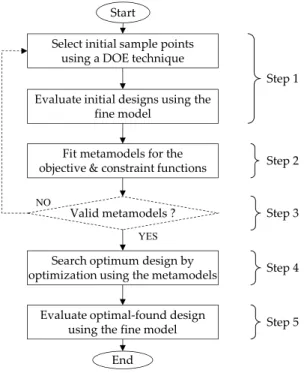
concepts which are later used within the optimization techniques and approaches developed and presented in the following chapters of the manuscript. The optimization process is only a phase, the core, of the three‐step optimal design process. Two other steps, equally important, a preliminary model analysis phase and a results interpretation and analysis, finalized with the decision making must also be accounted for within the optimal design process of complex systems.
The second chapter of the manuscript addresses a specific category of optimization techniques relevant for complex engineering design problems – the metamodel‐based design optimization approach. The simulation codes (FEA, CFD, etc.) are accurate tools for simulating the behavior of the device, allowing to account for complex physical phenomena which cannot be captured through analytical relations. The increased accuracy of these tools comes for the price of long computational time, a single evaluation of such a code taking between minutes, up to hours and even days, depending on the complexity of the model and the type of analysis required. The integration of such expensive simulations within a classical optimization process is thus prohibitive, due to the great number of successive calls of the optimization algorithm to the simulation model. For devices or systems represented by such simulation codes, a common practice consists in creating
metamodels, which benefit of a fast evaluation. The main issue with the metamodels represents the
accuracy of these representations. The integration of metamodels into the optimization process is discussed in this chapter and the purposes are sustained through both mathematical analytical test problems and a well‐known electromagnetic benchmark problem. These optimization techniques find application in the last chapter of the manuscript, which addresses the design optimization at a larger extent, considering a system as an ensemble of models or components.
The third chapter addresses the complex system optimization through means of decomposition of the system following different perspectives and the associated specific coordination techniques of the optimizations formulated for each element of the decomposed structure. Such optimization approaches represent a current practice in the automobile and aerospace industries, where they were developed and employed for more than a decade. The motivation of analyzing such optimization techniques for electromagnetic and railway applications comes from the great success that they have shown in the domains where they were introduced, showing a great potential. Several decomposition perspectives are reviewed, based on different models of the same device, the disciplines involved in the representation of the system and the different physical sub‐ systems and components of the complex system. First, the optimization of model‐based decomposed systems is introduced and addressed using a Space Mapping technique, Output Space
Mapping (OSM). A single‐phase safety isolation transformer benchmark is introduced as
application for this optimization technique. The OSM optimization approach makes use of two models of the same device, one being a high fidelity finite element model (3D FEM) and the other one a fast evaluation coarse analytical model with a limited fidelity. The synergies of the two models are exploited by the OSM algorithm, retrieving the optimal design with a much reduced call to the expensive high fidelity FE model of the transformer. Another decomposition‐based optimization approach considers the complex system by the different disciplines involved in analyzing the system. The most representative optimization technique of this category, the
Collaborative Optimization (CO) technique is introduced and its performance is analyzed through
application to the same transformer benchmark optimization problem previously mentioned. Another decomposition‐based optimization technique, this time considering the complex system through its sub‐systems and components is analyzed. The Analytical Target Cascading (ATC) is an
27
optimization technique which addresses the system decomposed into its sub‐systems and components, which are hierarchically displaced onto several levels, starting with the most global at the top of the hierarchy and the smallest component placed at the bottom level of the hierarchy. This technique was originally introduced as a specifications formalizing method, to cascade the system‐level targets down the hierarchy, to the most basic components. This optimization approach was already found to cope very well with the hierarchical organization of the Alstom Company and the way the system design specifications are imposed in the different departments of the company. The previous research studies of Moussouni [MOU 09a] and Kreuawan [KRE 08] have analyzed the basic configuration of this technique. The exploration of this technique is continued within this research study by going further into the functional mechanisms of the technique. A multi‐level railway test‐problem of Alstom Company, consisting in the optimal dimensioning of an ultra‐capacity energy storage system onboard a tramway, is introduced and used here as application of the ATC technique.
Chapter 1 Decision support tools for
complex electromagnetic systems design
In this chapter, the optimal design process is introduced and the general aspects of the complex system optimal design are addressed in general lines. The optimal design process is regarded as a three‐step process, consisting of a preliminary phase of problem definition, the main phase of optimization problem solving and a result analysis and decision making phase. The basic mathematical formulations of both the single‐ and the multi‐objective optimization are introduced and the notion of optimality in both the single‐ and the multi‐objective context is discussed. Some classical both deterministic and stochastic optimization algorithms are briefly presented for solving single‐objective optimization problems. Several techniques for transforming a multi‐objective optimization problem into a single‐objective problem are reviewed, which will be used later on within the advanced optimization techniques developed in the manuscript. A number of multi‐ dimensional data representation techniques, meant to assist the designer with the decision making, are presented towards the end of the chapter.
1.1 General aspects of an optimal design process
The optimal design approach of a device, product or system implies three main steps: ‐ Preliminary phase (problem formulation); ‐ Optimization process (algorithm run); ‐ Results visualization and analysis (decision making). These sequential steps are strongly related one to another and the result of the optimal design process depends on the appropriate addressing of all three steps. The brief description of these steps is presented next.Preliminary phase (optimization problem formulation)
The preliminary phase of the optimal design approach consists in acquiring and resembling all the necessary information about the device, system or process to be optimally designed. In this phase, the designer tries to gain as much information as possible about the object of his design, for this will help him to appropriately define the optimization problem to be solved. The result of the optimization process depends entirely on the formulation of the optimization purpose, therefore
the proper formulation of the optimization problem is crucial for the success of the optimal design process. A number of issues are addressed within this step, such as: the model (or models) of the device which are to be used within the optimization process, the parameters and design variables of the model, the type of design variables (continuous, discrete, unclassifiable), the domain of variation for the design variables, the output variables of the model, the type of optimization problem (linear, non‐linear), etc.
An important action at this stage consists in determining the kind of relationships existing between the input, output and input/output variables of the model, as well as the relative influence of the input variables over the outputs of the model (sensitivity analysis). The influence of the different design variables on the outputs of the considered model are analyzed with the goal of identifying those variables which do not (or have very little) influence upon the outputs of the model, so that they will be ignored in the formulation of the optimization problem. This way, the optimization algorithm is charged with determining the optimal values of only the influent parameters, thus alleging more or less considerably the task of optimization and saving important computational time. A few tools for the analysis of the functional relationships governing a model are presented later on, in paragraph 1.2.
Optimization process (algorithm run)
The second step of the optimal design process is represented by the optimization process itself, which represents the core of the optimal design process. Complex mathematical techniques are employed at this stage for solving the optimization problem previously formulated. During the last two decades, once with the strong development of the computational power and the appearance of the personal computers, a lot of research has been dedicated to the development of optimization algorithms and mathematical optimization techniques. These optimization algorithms make successive calls to the model of the device considered, selecting then new samples to be evaluated based on the values already calculated.
Depending on the type of optimization problem previously formulated, an appropriate optimization algorithm is selected to solve this problem. The optimization problems can be classified based on several different criteria. Thus, if the objective function can be expressed as a linear combination of the design variables, we deal with a linear optimization problem or linear programming. Otherwise, the problem is said to be non‐linear, solved using non‐linear programming techniques (NLP). If the design variables of the problem take discrete values, the optimization problem is discrete or combinatorial. A number of combinatorial techniques with application in electrical engineering are presented in [TRA 09]. If the domain of variation of variables is continuous, then the optimization problem is continuous. It often arrives that an optimization problem presents both continuous and discrete variables. In this case, it is employed the term of mixed‐integer optimization.
The optimization techniques developed and presented further on in Chapter 2 and Chapter 3 of this manuscript belong to the category of NLP techniques. Although several optimization applications addressed in this work have both discrete and continuous variables, in this work all variables of the applications are considered continuous and handled accordingly.
1.2 Variables influence and correlation 31
Results visualization and analysis (decision making)
The third and final step of the optimal design process is represented by the analysis and interpretation of the results supplied by the optimization process mentioned in the previous paragraph. When a multi‐objective formulation has been chosen for the optimization problem, the result is a set of optimal trade‐off designs between the considered objective functions. In this case, the final choice for the design to be considered remains at the latitude of the designer, engineers and/or managers, which will select one design to be conceived. Thus, the multi‐objective optimization represents a tool for decision‐making. A number of tools for the representation and visualization of the results, such as bar charts, spider diagrams, bubble plots, parallel coordinates representations, scatter plot matrix, etc. [EST 12], [NOE 12] have as goal to assist the designer with the decision‐making process. Some of these multi‐dimensional data representation techniques will be introduced later on in this chapter, in paragraph 1.4.2.
Now that the steps of the optimal design process were briefly described, the attention is turned to each of them at a time, starting with some means of analyzing the correlation between the variables of a model, in the preliminary phase of the optimal design process.
1.2 Variables influence and correlation
An important number of statistical analysis tools exist, assisting the designer in obtaining insights into the functional relationships between the variables of a model. Model analysis techniques and tools such as the screening technique [VIV 02], analysis of variance (ANOVA) [GOU 06], and response surface methodology are based on the realization of different experimental designs and represent notorious statistical tools. Therefore, these techniques will not be addressed here. Nevertheless, some techniques for the qualitative analysis of models, such as the Pearson correlation coefficient and the Spearman correlation coefficient represent powerful tools for gaining insights into the functional relationships of a model, being less employed currently. These coefficients will be next presented in the following paragraphs.
Pearson correlation coefficient
The Pearson correlation coefficient is a measure for the linear relationship between two input/output variables of a model [MAS 06]. The value of the coefficient is calculated based on a set of n samples , , for which the model has been run. Such a set of samples can be obtained using a design of experiments (DOE) technique [GOU 06], also known as experimental design. The value taken by this coefficient is always between ‐1 and 1. If the graphical representation of all pairs of samples is a straight line, it means that there is a strong linear correlation between the two variables. The slope of the straight line gives the sense of the correlation: positive slope gives positive value for the Pearson coefficient, respectively negative slope corresponds to a negative value of the Pearson coefficient. A value of zero for the Pearson correlation coefficient signifies that no linear correlation exists between the corresponding pair of variables of the model.
, ,
(1.1)
where represents the standard distribution of the values of the variable from the experimental design, represents the standard distribution of the values of and , represents the covariance between the two variables over the experimental design considered.
The expression of the covariance , between the two variables and is given in (1.2).
, 1
1 ̅ (1.2)
where ̅ represents the mean value of the variable over the experimental design considered and represents the mean value of .
Spearman rank correlation coefficient
The Spearman rank correlation coefficient [NAK 09], also known as Spearman’s rho [EST 12] is a non‐parametric statistical measure of the monotonicity of a function.
The first step in calculating the Spearman correlation coefficient consists in assigning to each value of the variables from the experimental design a rank, following a descending order, i.e.
1 where max , 1, ⋯ , .
As in the case of the Pearson coefficient, the value taken by the Spearman correlation coefficient is always between ‐1 and 1. A value close to 1 for this coefficient signifies that there is a strong direct correlation between the two variables, while a value close to ‐1 indicates a strong inverse correlation between the two variables. If the value of this coefficient is close to zero, then it means that no correlation exists between the two variables. However, in this latter case, a non‐monotonic correlation may exits. The expression of the Spearman correlation coefficient is given in (1.3). , ∑ ∙ ∑ ∙ ∑ (1.3)
where represents the mean value of the ranks of all values of the variable, calculated according to (1.4).
1
(1.4)
Correlation matrix
The correlation matrix or correlation chart [EST 12] represents a graphical tool for visualizing the values of different correlation coefficients. Once a correlation coefficient (Pearson, Spearman or other) is calculated for every pair of input/output variables of a model, these values can be represented under a matrix form. This way, the strong correlations between variables can be easily
1.2 Variables influence and correlation 33
detected, as well as variables which present a negligible correlation, being therefore considered uncorrelated. A correlation matrix tool, inspired from the correlation chart of the modeFRONTIER commercial optimization software product [EST 12], has been developed under Matlab®.
To exemplify the purpose of the correlation coefficients, a simple model consisting of four mathematical analytical relations depending on two variables is considered in (1.5). 4 4 (1.5) 1 2 4 1 with , ∈ 4,4
For the model expressed in (1.5), a design of experiments of 20 designs has been considered using the Latin Hypercube Sampling (LHS) methodology. The LHS technique, introduced by McKay et al. in [MCK 00] is very popular experimental design for computer experiments [KRE 08].
The correlation coefficients for the model considered in (1.5) have been calculated and represented using the correlation matrix shown in Figure 1.1. a) Pearson correlation coefficients b) Spearman correlation coefficients Figure 1.1 : Correlation matrix Similar values for the two correlation coefficients, Pearson and Spearman, have been obtained, as can be seen from Figure 1.1a and Figure 1.1b. In complement to the correlation coefficients, the strong correlations are represented using dark blue or red colors (for negative, respectively positive correlations), while the low correlations have a faded color. From these two correlation charts, it can be seen the level of correlation between the variables of the model ( , ) and the outputs ( , , , ). For example, a complete linear inverse correlation is immediately detected for the couple , . Also, a strong linear correlation is observed between and , which is logic if we take a look at the expression of in (1.5). Another remark is that although both and variables are present in the expression of , due to the quadratic terms, is almost completely correlated with , while no correlation is detected between and . The
correlation matrix presents itself as an easy mean of empirically validating the tendencies of the functional relationships of a model.
Once reviewed the correlation matrix as a tool for the empirical model validation prior to the optimization process run, the basic mathematical formulations of both the single‐ and the multi‐ objective general optimization problems are introduced next.
1.3 Single and multi‐criteria optimization
Most of the real life optimization problems are multi‐objective by their nature. However, the optimization problem can be expressed using a unique objective (single‐objective optimization) or several criteria can be accounted for within the expression of the optimization problem. The optimization problems may or may not present constraint functions (constrained or unconstrained optimization). There are next introduced some elementary notions about a single‐objective optimization problem formulation.
1.3.1 Single‐objective optimization
The general mathematical formulation [VEN 01] of a single‐objective constrained optimization problem is expressed in (1.6). Minimize (1.6) subject to 0 1, ⋯ , 0 1, ⋯ , with , ⋯ , , ⋯ , 1, ⋯ ,
where represents the vector of design variables, each variable being defined between a lower and an upper bound, respectively , also known as “box constraints”, represents the objective function to be minimized1, represents the i‐th inequality constraint function, represents the j‐th
equality constraint function, represents the number of design variables, represents the number of inequality constraint functions and represents the number of equality constraint functions of the optimization problem.
Within the formulation of an optimization problem, the equality and/or inequality constraint functions might be absent. If both equality and inequality constraint functions are lacking, the optimization problem is said to be “unconstrained”. However, rare is the case in practical applications where no constraint functions are formulated within the optimization problem.
1 The convention generally adopted by the research community expresses any optimization problem as a minimization
problem. When the optimization problem implies an objective function to be maximized, this is represented within the general formulation of the optimization problem by using the minus sign (Maximize ≡ Minimize ).
1.3 Single and multi‐criteria optimization 35
1.3.2 Local vs. global optimality
Two different types of optima exist in the resolution of a nonlinear optimization problem. These are illustrated graphically using an abstract single‐dimensional continuous example function presented in Figure 1.2.
A point ∗ is a local minimum of the function if the expression (1.7) is valid [MES 07].
∗ ∀ ∈ ∗ , ∗ , ∗ ⊂ , ⊂ (1.7)
where ∗ is a subdomain of , the domain of definition of the function, defining the neighborhood of the point ∗.
The function may have several local optima (minima).
A point ∗ is a global minimum of the function if the expression (1.8) is respected.
∗ ∀ ∈ , ∗ , ⊂ (1.8) As in the case of the local optima, several global optima (minima) of the function may exist. The uniqueness of the global solution is guaranteed if the relation (1.9) is respected. ∗ ∀ ∈ , ∗ , ⊂ (1.9) Hence, the global optimum of a function is necessarily also a local optimum of the function. The reverse statement is obviously not true. Figure 1.2 : Local vs. global optimality representation The example function presented in Figure 1.2 shows three distinct local optima (minima),
∗, ∗ and ∗. Among these local minima, the function presents only one global minimum, ∗,
since ∗ , ∀ ∈ , .
The main difficulty faced by an optimization algorithm is to avoid being caught in a local basin of attraction of the function to be optimized.