Biodegradation of chloroacetanilide herbicides in wetlands

(1)

HAL Id: tel-01280603

https://tel.archives-ouvertes.fr/tel-01280603

Submitted on 29 Feb 2016

HAL is a multi-disciplinary open access archive for the deposit and dissemination of sci-entific research documents, whether they are pub-lished or not. The documents may come from teaching and research institutions in France or abroad, or from public or private research centers.

L’archive ouverte pluridisciplinaire HAL, est destinée au dépôt et à la diffusion de documents scientifiques de niveau recherche, publiés ou non, émanant des établissements d’enseignement et de recherche français ou étrangers, des laboratoires publics ou privés.

Biodegradation of chloroacetanilide herbicides in

wetlands

Omniea Elsayed

To cite this version:

Omniea Elsayed. Biodegradation of chloroacetanilide herbicides in wetlands. Ecosystems. Université de Strasbourg, 2015. English. �NNT : 2015STRAJ003�. �tel-01280603�

(2)

UNIVERSITÉ DE STRASBOURG

ÉCOLE DOCTORALE des sciences de la Vie et de la Santé

UMR 7156 UNISTRA - CNRS

Génétique Moléculaire, Génomique, Microbiologie (GMGM)

THÈSE

présentée par :

Omniea ELSAYED

Biodegradation of chloroacetanilide herbicides

in wetlands

soutenue le : 23 Janvier 2015

pour obtenir le grade de:

**!"#$%&'($')*%+,-$&.,#/'($'0#&1.2!%&3**

Discipline: Sciences du Vivant

Spécialité : Aspects moléculaires et cellulaires de la biologie

THÈSE dirigée par :

M. IMFELD Gwenaël Chargé de recherche, CNRS, Université de Strasbourg, France M. VUILLEUMIER Stéphane Professeur, Université de Strasbourg, France

RAPPORTEURS :

M. BAYONA Josep M Professeur, IDAEA, Espagne

M. TRUU Jaak Professeur, Université de Tartu, Estonie AUTRES MEMBRES DU JURY :

M. MILLET Maurice Professeur, Université de Strasbourg, France Mme. NIJENHUIS Ivonne Senior scientist, UFZ, Allemagne

(3)

(4)

III

!"#$%"&'"(")+,-./0"-1"("2.'1&-(1&-3*

(5)

IV

Acknowledgments

The work of this PhD thesis was performed at the Laboratory of Hydrology and Geochemistry of Strasbourg (LHyGeS)!" #$% 7517-CNRS-Université de Strasbourg, and the laboratory &'(')*+,-"$./'0,/1*2-3"Génomique, Microbiologie (GMGM)!"#$% 7156-CNRS-Université de Strasbourg. Thanks to all the members of both laboratories. This PhD work was funded by the European Union under the 7th_{Framework Programme (Marie Curie Initial Training}

Network CSI:Environment, Contract Number PITN-GA-2010-264329).

Thank you Dr. Gwenael Imfeld and Prof. Stéphane Vuilleumier, directors of this PhD thesis for their continuous support and guidance, especially during the last year. Gwenaël3"456"7-28" grateful for the moral support and encouragement during the ups and downs (and there has been many) of this four year long journey. 456" 7-28" 921)-:,/" )." ;)'<=1(-" :.2" <.*()*(9" 6-" towards this PhD position when I first contacted him more than four years ago, it was a great opportunity for me. I would also like to thank you both for the time and effort spent on corrections and feedback of different parts of this manuscript.

I would also like to thank members of my PhD jury: Prof. Josep M Bayona, Prof. Jaak Truu, Dr. Ivonne Nijenhuis and Prof. Maurice Millet for kindly accepting to evaluate my work.

I would like to thank Dr. Ivonne Nihenhuis and all the members of the Isotope biogeochemistry in the Helmholtz Centre for Environmental Research > UFZ in Leipzig for welcoming me in your lab and helping me with the CSIA measurements. A special thanks to Mathias Gehre, Ursula Günther and Falk Bratfisch for their help with the IRMS machines (Benny). My heartfelt thanks to Sara Herrero Martin for advice and support during my stay in Leipzig and through all different organisational aspects of CSI:Environment project.

My PhD experience was a bit particular in that I had two offices, two teams and two supervisors. This experience was overall enriching, though challenging at times. This work ?.,/@(5)"=17-"A--("<.BB*A/-"?*)=.,)")=-"=-/<"1(@"B,<<.2)".:"6-6A-2B".:"A.)=")-16B at the LHyGes and the GMGM. Thanks to Elodie, Marie, Ivan, Benoit, Clio and Izabella in the LHyGeS not only for the good cooperation and scientific discussions but also for their

(6)

V welcome to the team and for the effort you made to speak in English when I first started in the /1A3"1/)=.,9="*)"@*@(5)"/1B)"/.(9C Thank you Nicolas Trottier and Yi for being great office-mates. 456"1/B."7-28"921)-:,/")."D-(.*)"1(@"E2*0":.2")=-*2")-0=(*01/"=-/<"*(")=-"/1A"1(@"9..@"0.6<1(8C"" I also thank all 3rd_{floor PhD students for always keeping a good atmosphere in the lab. I am}

lucky to have you all as friends and as colleagues. Thanks to all members of the LHyGeS for /-B").,2(.*B"@-"<')1(+,-!"1(@" /-B"fêtes @-"/1"6.,B)10=-!"?=*0="?-2-"1/?18B"1"/.)".:":,(C"F(" the other side (GMGM) I thank Christelle and Yousra for guiding me to through the tips and tricks of the lab and for preparing the agarose gels for me during the last two months of lab-work. Thank you Thierry for always accepting to help with different bits of lab-work with a welcoming attitude. Thank you Françoise for the continuous good energy and cheerfulness, it always helped to lift my mood. Thank you Farhan for showing me how things are done when I first started doing lab work at the GMGM. Thanks to all PhD students at the GMGM: Pauline, Farah who were always a good company. I also wish to express my gratitude to all the trainees who helped in different parts of this work, especially Renata, Ana and Julie. Your contributions were very valuable to my work.

To all CSI:Environment fellows: thanks for your friendship, for your cooperation and the good times we had together touring Europe while learning about isotopes!

A final and big thank you goes to my family who have encouraged me to start this project and supported me all the way. Thank you Adham for always being there and for believing in me. Thank you baby Donya for bearing up with me through the final phases of write-up and helping me keep things in perspective. My deep thanks goes to all who enjoyed the company of Donya to allow me to finish this manuscript (mama, Noura & Hend).

(7)

VI

Remerciements

Ce travail de thèse a été réalisé au Laboratoire d'Hydrologie et de Géochimie de Strasbourg (LHyGeS) UMR 7517 CNRS-Université de Strasbourg, et dans l'unité de recherche Génétique Moléculaire, Génomique, Microbiologie (GMGM) UMR 7156 Université de Strasbourg - CNRS. Merci à tous les membres de ces deux laboratoires. Ce travail de thèse a été financé par l'Union européenne au titre du 7éme programme-cadre (Réseau de formation initiale Marie Curie, CSI: Environnement, contrat Nombre PITN-GA-2010-264329).

Merci Dr. Gwenaël Imfeld et Prof. Stéphane Vuilleumier, directeurs de ce travail de doctorat pour leur soutien et leur supervision, en particulier au cours de la dernière année. Dr. Imfeld, je suis très reconnaissante pour ton soutien moral et tes encouragements pendant les hauts et les bas (et il y en a eu beaucoup) de ce voyage de quatre ans. Je suis très reconnaissante au G2.:C"H,*//-,6*-2"<.,2"6517.*2".2*-()'"7-2B"0-))-"<.B*)*.("@-"@.0).21)"+,1(@"I-"/J1*"0.()10)'"*/" 8" 1" </,B" @-" +,1)2-" 1(B3" -)" +,*" B5-B)" 2'7élée être une grande opportunité pour moi. Je tiens également à vous remercier tous les deux pour le temps et les efforts consacrés aux corrections -)"K"/5'71/,1)*.("@-B"@*::'2-()-B"<12)*-B"@-"0-"61(,B02*)C

Je tiens également à remercier les membres de mon jury de thèse: Prof. Josep M Bayona, Prof. L11M"N2,,3"O2C"47.((-"P*I-(=,*B"-)"G2.:C"$1,2*0-"$*//-)"@517.*2"A*-("7.,/,"100-<)-2"@J'71/,-2" mon travail de thèse.

L-")*-(B"K"2-6-20*-2"O2C"47.((-"P*=-(=,*B"-)").,B"/-B"6-6A2-B"@-"/5'+,*<- biogéochimie des isotopes dans le Centre Helmholtz pour la recherche environnementale - UFZ de Leipzig de 6517.*2"100,-*//*-"@1(B"7.)2-"/1A.21).*2-"-)"@-"6517.*2"1*@'"17-0"/-B"1(1/8B-B"Q;4RC"#("921(@" merci à Mathias Gehre, Ursula Günther et Falk Bratfisch pour leur aide avec la machine IRMS (Benny). Mes sincères remerciements à Sara Herrero Martin pour tous les conseils et le soutien pendant mon séjour à Leipzig ainsi que son aide pour tous les différents aspects organisationnels du projet CSI: Environnement.

Mon expérience d-" @.0).21)" ')1*)" <12)*0,/*S2-" ')1()" @.(('" +,-" I5171*B" @-,T" A,2-1,T3" @-,T" équipes et deux directeurs de thèse. Cette expérience a été stimulante et enrichissante. Ce )2171*/" (51,21*)" <1B" ')'" <.BB*A/-" B1(B" /J1*@-" -)" /-" B.,)*-(" @-B" 6-6A2-B" @-B" @-,T" '+,*<-B" 1, LHyGes et au GMGM. Merci à Elodie, Marie, Ivan, Benoît, Clio et Izabella au LHyGeS non seulement pour le bon travail en collaboration et pour les discussions scientifiques

(8)

VII globale de ce doctorat. Merci pour l'accueil chaleureux de toute l'équipe et pour l'effort que 7.,B"17-U":1*)"@-"<12/-2"-("1(9/1*B"+,1(@"I51*"0.66-(0'"@1(B"/-"/1A.21).*2-3"6V6-"B*"0-/1"(J1" pas duré très longtemps . Merci Nicolas Trottier et Yi Pan pour avoir été de merveilleux « co-bureau ». Je suis également très reconnaissante à Benoît Guyot et à Eric Pernin pour leur aide technique dans le laboratoire et leur bonne compagnie. Je remercie également tous les @.0).21()B"@,"WS6-"')19-"@517.*2"912dé toujours une bonne ambiance dans le laboratoire. Je suis très heureuse de vous avoir comme amis et collègues. Merci à tous les membres du LHyGeS pour la convivialité "des tournois de pétanque" et "des fêtes de la moustache". Du côté (GMGM), je remercie Christelle Gruffaz et Yousra Louhichi pour leurs aides précieuses et leurs conseils pratiques pour le travail au laboratoire et spécialement pour leur assistance à la préparation des gels d'agarose pendant les deux derniers mois de manips. Merci à Thierry P1@1/*9" @517.*2" ).,I.,2B" 100-<)'" @-" 651*@-2" :1*2-" /-B" 61(*<B" 17-0" 9-()*//-BB-C" $-20*" K" X21(Y.*B-"D2*(9-/"<.,2"B.("'(-29*-"-)"B1"A.((-"=,6-,23"+,*"65.()").,I.,2B"1*@'"K"912@-2"/-" 6.21/C" $-20*" K" $,=1661@" X12=1(" #/" Z1+,-" <.,2" 6517.*2" 9,*@'" 1," @'612219-" +,1(@ I51*" commencé à faire des manips au GMGM. Merci à tous les doctorants au GMGM: Pauline et X121=C"L-")*-(B"'91/-6-()"K"-T<2*6-2"61"921)*),@-"K").,B"/-B"B)19*1*2-B"+,*"65.()"1*@'"@1(B"/-B" différentes parties de ce travail, en particulier Renata, Ana et Julie. Vos contributions ont été très précieuses pour mon travail.

A tous les doctorants dans le réseau CSI: Environnement: merci pour votre amitié, votre coopération et les bons moments que nous avions passés ensemble partout en Europe, tout en découvrant les isotopes!

X*(1/-6-()3",(")2SB"921(@"6-20*"K"61":16*//-"+,*"651"-(0.,219'"K"0.66-(0-2"0-"<2.I-)"-)" 651"B.,)-(,").,)"1,"/.(9"@,"0=-6*(C"$-20*"R@=16"@JV)2-").,I.,2B"/K"-)"@-"02.*2-"-("6.*C"$-20*" A'A'"O.(81"@517.*2"B,<<.2)'"/-B"<=1B-B":*(1/-B"@-"/1"2'@10)*.("@-"/1")=SB-"-)"@-"6517.*2"1*@'"K" garder les choses en perspective et merci à tous ceux qui ont gardé Donya pour me permettre de terminer ce manuscrit (maman, Noura et Hend).

(9)

VIII

Résumé étendu

La biodégradation de chloroacétanilides dans les zones humides

Introduction

Les chloroacétanilides (métolachlore, alachlore et acétochlore ; Figure I) sont une famille d'herbicides largement utilisés pour le contrôle des graminées annuelles et des mauvaises herbes sur une grande variété de cultures, notamment maïs, tournesol et betterave sucrière (Pereira et al., 2009). Les chloroacétanilides sont des herbicides de pré-/-7'-" [05-B)-à-dire appliqués avant le développement du couvert végétal), dont la solubilité élevée dans l'eau les 2-(@B" <12)*0,/*S2-6-()" B,I-)B" K" ,(-" 6.A*/*B1)*.(" /.2B" @5'7'(-6-()B" 2,*BB-/1()B" [%-*@" et al., 2000). Les chloroacétanilides et leurs produits de dégradation sont ainsi fréquemment détectés comme contaminants dans les nappes phréatiques et les eaux de surface, soulevant des interrogations quant à leurs impacts sur les écosystèmes et la santé humaine (Baran et Gourcy, 2013).

Figure I. Structure moléculaire des herbicides métolachlore, acétochlore et alachlore. La

structure moléculaire commune des chloroacétanilides est mise en évidence en bleu clair.

La compréhension des processus de transport et de dégradation régissant le devenir des pesticides est donc essentielle pour l'optimisation de stratégies de remédiation et une meilleure évaluation des risques environnementaux de contamination par les pesticides. Cependant, les processus régissant le transport et la biodégradation des chloroacétanilides en terres agricoles, en passan)" <12" /-B" U.(-B" 2'10)*7-B3" )-//-B" +,-" /-B" U.(-B" =,6*@-B3" -)" 0-" 171()" @51))-*(@2-" /-B" écosystèmes aquatiques, restent mal connus. Les zones humides sont des écosystèmes dans lesquelles une grande variété de processus permettent la dégradation des pesticides (Stehle et

(10)

IX bactériennes et les processus biogéochimiques actifs dans les zones humides (Borch et al., 2010). La biodégradation est considérée actuellement comme le principal processus de transformation des chloroacétanilides dans l'environnement (Fenner et al., 2013), tandis que /-B" )21(B:.261)*.(B" 1A*.)*+,-B3" )-/B" +,-" /1" <=.)./8B-" .," /5=8@2./8B-3" B-6A/-nt jouer un rôle mineur (Zhang et al., 2011). Parallèlement, la composition et le fonctionnement microbiens sont impactés par l'exposition aux pesticides (Imfeld et Vuilleumier, 2012). Potentiellement, les communautés microbiennes représentent ainsi des bio-indicateurs de l'exposition aux pesticides dans les zones humides (Sims et al., 2013). Cependant, la connaissance des communautés microbiennes associées à la dégradation des chloroacétanilides dans les zones humides, et les paramètres environnementaux associés est encore rudimentaire.

Traditionnellement, les études sur l51))'(,1)*.(" @-B" <-B)*0*@-B" @1(B" /-B" U.(-B" =,6*@-B" consistent en des bilans massiques entrée-sortie des pesticides, et portent rarement sur les processus de dégradation in situ. Dans le cas des chloroacétanilides, une grande variété de processus de dégradation peut être envisagée, bien que les connaissances sur les conditions dans lesquelles chaque processus est pertinent sont encore limitées, et les approches pour l'évaluation de la dégradation in situ de chloroacétanilides manquent largement. De nouvelles approches expérimentales peuvent fournir un aperçu sur les processus de dégradation in situ des pesticides. Celles-ci comprennent notamment l'analyse isotopique composé-spécifique (CSIA) et l'analyse chirale (Milosevic et al., 2013), ainsi que les techniques moléculaires de l'écologie microbienne. Avant le début de la présente thèse, ces différentes approches n'avaient <1B"')'"@'7-/.<<'B".,"1<</*+,'B"@-"0.(I.*()-6-()"-)"@-":1Y.("0*A/'-"K"/5'),@-"@-"/1"dégradation des chloroacétanilides dans les zones humides.

Objectifs du projet de doctorat

L'objectif général de la thèse a été d'évaluer la dégradation in situ des chloroacétanilides, et de caractériser la diversité bactérienne associée dans les zones humides. Les objectifs spécifiques de cette thèse étaient les suivants:

\" @'7-/.<<-2" -)" 71/*@-2" ,(-" 6')=.@-" Q;4R" <.,2" '71/,-2" /1" @'921@1)*.(" in situ @5=-2A*0*@-B" chloroacétanilides dans l'environnement;

\"B,*72-"/-B"0.66,(1,)'B"A10)'2*-((-B"1BB.0*'-B"K"/1"@égradation des chloroacétanilides à l'aide d'outils moléculaires;

(11)

X \"'71/,-2"/1"@'921@1)*.("in situ de chloroacétanilides dans les zones humides et sa relation avec les conditions biogéochimiques;

\"'71/,-2"/J*6<10)"@-B"0.(@*)*.(B"=8@21,/*+,-B"-)"@,"6.@-"d'exposition aux herbicides sur la biogéochimie, la dissipation des chloroacétanilides et sur les communautés bactériennes dans les zones humides.

Des zones humides expérimentales ont été choisies comme systèmes-modèles pour étudier le devenir de chloroacé)1(*/*@-B"@1(B"@-B"0.(@*)*.(B"@8(16*+,-B"@5.T8@.-réduction. Ces zones humides expérimentales intègrent les principales caractéristiques des zones humides (par exemple les interactions de sédiments, eau et plantes), tout en permettant un meilleur contrôle des paramètres environnementaux (par exemple les flux de contaminants), et donc une meilleure interprétation des processus de dégradation in situ. Plusieurs outils ont été développés et combinés pour étudier la dégradation de chloroacétanilides dans les zones humides étudiées. O-B"6')=.@-B"@51(1/8B-"=8@2.9'.0=*6*+,-"-)"1(1/8)*+,-".()"')'"1<</*+,'-B"K"/5'),@-"@,"/*-(" -()2-"/-B"0.(@*)*.(B"A*.9'.0=*6*+,-B"-)"/1"@'921@1)*.("@-B"0=/.2.10')1(*/*@-BC"]51(1/8B-"Q;4R3" l'analyse des produits de dégradation et (dans le 01B"@-"6')./10=/.2-^"/51(1/8B-"@-"0=*21/*)'".()" été utilisées pour démontrer la dégradation des chloroacétanilides in situ, et pour fournir des indications sur les processus impliqués. Le génotypage T-RFLP et le pyroséquençage 454 ont été utilisés pour caractériser la diversité des communautés bactériennes dans les zones humides 0.()16*('-B" <12" /-B" 0=/.2.10')1(*/*@-B3" -)" @')-26*(-2" /-,2" 2'<.(B-" K" /5-T<.B*)*.(" 1,T" chloroacétanilides et aux conditions hydrochimiques.

Résumé des résultats obtenus au cours du projet de doctorat

La transport et la dégradation des chloroacétanilides ont d'abord été étudiés dans des zones humides à écoulement vertical au laboratoire, pour mieux comprendre les processus de dégradation du métolachlore, de l'acétochlore et de l'alac=/.2-"K"/5*()-2:10-".T*+,-_1(.T*+,-" dans les zones humides, et leur lien avec les communautés bactériennes aquatiques (Elsayed et al.3"`abcA^C"]1"@*6*(,)*.("@-"0=129-"@510').0=/.2-"-)"@J1/10=/.2-"-()2-"/J-()2'-"-)"/1"B.2)*-"@-B" zones humides ont été respectivement de 56 et 51%, alors que le métolachlore s'est montré plus persistant, avec seulement 23% de dissipation. Ceci suggère que les différences structurelles entre les trois chloroacétanilides semblent déterminer en partie leur dégradation. La dégradation des trois chloroacétanilides s'est produite en particulier dans la rhizosphère, en

(12)

XI

Figure II. Concentrations d'accepteurs terminaux d'électrons (AFE) : oxygène (cercles noirs), nitrate (triangles gris) et sulfate (carrés blancs) dans les zones humides !"#$%& '()* +,-.'()&%'#+,")$,* ,&#(.*)-/*.$ ,0123,*4)-#(.-/*.$ ,0523, (,*4)*)-/*.$ ,0623, et (D) par le contrôle sans herbicide. Les concentrations relatives des chloroacétanilides (Cx

/ Cin = concentration au point (x) divisée par la concentration d'entrée) aux différentes

profondeurs des zones humides de laboratoire sont indiquées par des barres grises, comme la moyenne ± écart-type [d"e"f^"@-"/5-(B-6A/-"@-B"71/-,2B".A)-(,-B").,)"1,"/.(9"@-"/5-T<'2*-(0-C

(13)

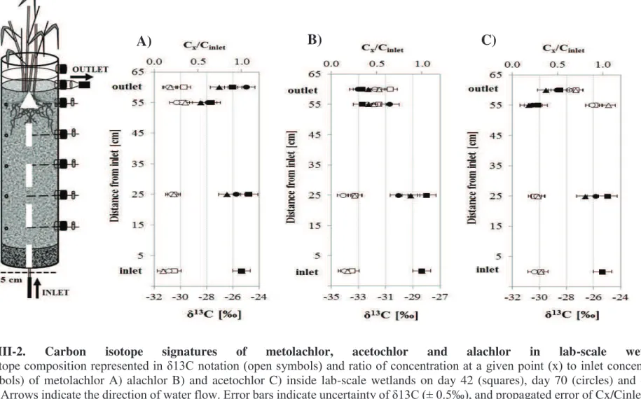
XII #(-" 6')=.@-" @51nalyse isotopique composé-spécifique (carbone) du métolachlore, de /51/10=/.2-"-)"@-"/510').0=/.2-"@1(B"/-B"'0=1()*//.(B"@J-1,"1"')'"@'7-/.<<'-C"#(":210)*.((-6-()" isotopique prononcé a été observé (Figure III), suggérant une biodégradation in situ de l'ala0=/.2-"[gbulk = -`3a"e"a3W^"-)"@-"/510').0=/.2"[gbulk = -3,4 ± 0,5).

Malgré une faible dissipation, les rapports énantiomériques du métolachlore diffèrent entre la zone oxique (0,494 ± 0,006) et la zone rhizosphérique (0,480 ± 0,005), indiquant la biodégradation préférentielle de l'énantiomère S. Les paramètres hydrochimiques, et en particulier la concentration en oxygène, corrèlent avec les profils bactériens, contrairement aux concentrations en chloroacétanilides.

La rhizosphère était dominée par des bactéries Gram-positives anaérobies affiliées aux Clostridia et aux Actinobacteria, et par des Proteobacteria. Des taxons connus pour leur capacité à réduire le sulfate comme Deltaproteobacteria (Desulfobacteraceae, Desulfovibrionaceae, et Desulfobulbaceae) et Clostridium (Peptococcaceae) ont également été détectés. Les communautés bactériennes de la rhizosphère anoxique ont probablement contribué à la dégradation des chloroacétanilides, soit directement en catalysant leur biodégradation, soit en fournissant des molécules soufrées agissant comme des nucléophiles avec les chloroacétanilides. Les résultats obtenus soulignent l'importance de la dégradation 1(1'2.A*-"@-B"0=/.2.10')1(*/*@-B3"-)"*//,B)2-()"/-"<.)-()*-/"@5.,)*/B"*((.71()B")-/B"+,-"/-"Q;4R" -)"/51(1/yse énantiomérique, en combinaison avec des approches plus traditionnelles comme les analyses hydrochimiques, la quantification de pesticides et les analyses de produits de dégradation, pour évaluer le devenir des chloroacétanilides dans les zones humides.

(14)

XIII

Figure III. Signatures isotopiques du carbone du métolachlore, de l'acétochlore et de l'alachlore dans les zones humides expérimentales.

La composition *B.).<*+,-" @-" 012A.(-" -B)" 2-<2'B-()'-" -(" (.)1)*.(" h13C (symboles blancs) et C

x / Cin: concentration au point (x) divisée par la

concentration d'entrée (symboles noirs) de métolachlore en A) alachlore en B) et acétochlor en C) à l'intérieur des zones humides en colonnes le jour 42 (carrés), le jour 70 (cercles) et le jour 98 (triangles). Les flèches indiquent la direction d'écoulement de l'eau. Les barres d'erreur indiquent /J*(0-2)*),@-"@-"h13Q"[e"a3i"j^"-)"/J-22-,2"<2.<19'-"@-"Qx/Cinlet sur la base des écarts-types des concentrations.

(15)

XIV Le régime hydraulique joue également un rôle majeur dans l'évolution biogéochimique des zones humides et influence la dégradation des contaminants organiques, y compris les pesticides (Faulwetter et al., 2009). Dans un deuxième volet de ce travail, l'impact des conditions hydrauliques et le mode d'exposition aux herbicides sur les conditions biogéochimiques, la dissipation des chloroacétanilides, et la diversité des communautés bactériennes associées a été évalué, et le transport du S-métolachlore a été suivi dans une zone humide expérimentale à ciel ouvert (Elsayed et al., 2014a). L'influence des conditions hydrauliques et hydrochimiques sur la dégradation du S-métolachlore et sur les communautés bactériennes a été caractérisée dans deux zones humides artificielles identiques, imitant pour /5,(-" @-B" 0.(@*)*.(B" @5-T<.B*)*.(" 0=2.(*+,-" -)" 0.()*(,-" [:/,T" 0.()*(,^3" -)" <.,2" /51,)2e une exposition aiguë et transitoire au S-métolachlore (bâchées).

Les deux zones humides ont montré des conditions d'oxydo-réduction distinctes, correspondant aux différents régimes hydrauliques appliqués. La zone humide à écoulement continu se distinguait par des conditions anaérobies (potentiels redox variant de -190 mV à -400 mV), tandis que le système de traitement en discontinu alternait entre conditions aérobes et anaérobes (320 mV à -400 mV). Une réduction des nitrates, du manganèse et des sulfates a été observée dans les deux zones humides, mais de manière généralement plus prononcée dans la zone =,6*@-".<'2'-"-("Ak0='-BC"O-"6V6-3"/51))'(,1)*.("@-"S-métolachlore était plus élevée dans le système en bâchées (93-97%) que dans celui en flux continu (40-79%), en accord avec des études précédentes décrivant une activité biogéochimique et une élimination des contaminants organiques plus élevées dans les systèmes alternant les phases de saturation et d'insaturation que dans les zones humides saturées en continu et fonctionnant à faible potentiel redox (Avila et al., 2013; Dytczak et al., 2008).

Les différences de composition bactérienne observées dans les deux systèmes étaient modestes bien que significatives (p = 0,008), et une corrélation entre le S-métolachlore, les nitrates, et les concentrations totales de carbone inorganique a été notée (Figure IV). La composition bactérienne des eaux interstitielles des zones humides a évolué graduellement au fil du temps dans les zones humides à flux continu, et plus brusquement dans la zone humide en discontinu, reflétant les conditions distinctes de fonctionnement hydraulique et de potentiel redox dans les deux systèmes (Figure V). Les résultats obtenus suggèrent que les profils de composition bactérienne et leur dynamique pourraient servir comme bioindicateurs de l'exposition aux herbicides et aux perturbations hydrauliques dans les zones humides

(16)

XV

Figure IV. Représentation 2D-NMDS des profils des communautés bactériennes basée sur (A) la T-RFLP et (B) le pyroséquençage de la région hypervariable V1-V3 du gène ARNr 16S des échantillons d'eau de zones humides et de la rhizosphère. Les symboles sont libellés par

jour d'échantillonnage (jours 0, 35, 42, 56 et 77). 1m, 2m, 3m: 1, 2 et 3 mètres de l'entrée, respectivement. En (A), les vecteurs correspondent aux variables qui corrèlent significativement avec la structure de la communauté bactérienne (temps, S-métolachlore, nitrate, nitrite et carbone inorganique total). Stress : (A) 0,18%, (B) 0,04%

(17)

XVI

Figure V. Abondance relative [%] des classes bactériennes dominantes (seuil d'identité de séquence = 80%) dans les échantillons d'eau des zones humides pour les différents jours d'échantillonnage (jours 0, 35 et 56) ainsi que dans les échantillons de la rhizosphère. Les

(18)

XVI prévalent des conditions biogéochimiques dans le devenir des chloroacétanilides. L'importance des conditions anaérobies pour la dégradation de chloroacétanilides dans des environnements rédox-@8(16*+,-B" 1"')'" @'6.()2'-C"O-"</,B3"0-")2171*/"1"6*B"-("'7*@-(0-"/1"71/-,2"@5.,)*/B" *((.71()B" )-/B" +,-" /-" Q;4R3" /51(1/8B-" @'énantiomères, et l'analyse moléculaire de l'ADN -(7*2.((-6-()1/" <.,2" 01210)'2*B-2" /-" @-7-(*2" @5=-2A*0*@-B" 0=/.2.10')1(*/*@-B" @1(B" l'environnement.

En perspective de ce travail, la détermination de facteurs d'enrichissement isotopique des chloroacétanilides dans différentes conditions d'oxydo-réduction ainsi que l'identification de souches bactériennes dégradant les chloroacétanilides permettront d'améliorer la compréhension mécanistique des voies de dégradation de chloroacétanilides et des gènes cataboliques correspondants. L'application de ces approches expérimentales complémentaires contribuera à améliorer l'évaluation de la biodégradation des chloroacétanilides dans des environnements contaminés, et de mieux prédire à long-terme le devenir de pesticides en évaluant les risques environnementaux associés. Du point de vue de la remédiation, l'amélioration des connaissances sur la dégradation des chloroacétanilides servira également à l'optimisation de la conception de zones humides artificielles pour le traitement et l'élimination des chloroacétanilides et de micropolluants similaires.

(19)

XVII

List of Abbreviations

(Q)-ToF Quadrupole time-of-flight mass spectrometry

2,4-D 2,4-Dichlorophenoxyacetic acid

AKIE Apparent kinetic isotope effect ANOSIM Analysis of similarities

ANOVA Analysis of variance

BLAST Basic local alignment search tool

BTEX Benzene, toluene, ethylbenzene, and xylenes

CA Correspondence analysis

CCA Canonical correspondence analysis

CSIA Compound-specific isotope analysis

DCM Dichloromethane

DDT Dichlorodiphenyltrichloroethane

DEET N,N-Diethyl-meta-toluamid

DGGE Denaturing gradient gel electrophoresis

DMSO Dimethyl sulfoxide

DNA Deoxyribonucleic acid

dNTP Deoxyribonucleotide triphosphate

EA-IRMS Elemental analyzer-isotope ration mass spectrometry

EE Enantiomeric excess

EF Enantiomer-fraction

ESA Ethane sulfonic acid

ESIA Enantiomer-specific isotope analysis

GC Gas chromatography

GC-C-IRMS Gas chromatography-combustion-isotope ratio mass spectrometry

GSH Glutathione

GST Glutathione S-transferase

HESI Heated electrospray ionization

HRMS High resolution mass spectrometry

KIE Kinetic isotope effect

LC Liquid chromatography

LC-IRMS Liquid chromatography-isotope ratio mass spectrometry MAFFT Multiple alignment using fast fourier transform

MRM Multiple reaction monitoring

MTBE Methyl tertiary-butyl ether

NMDS Nonmetric multidimensional scaling

OTU Operational taxonomic unit

OXA Oxanilic acid

PCA Principle component analysis

PCoA Principle coordinate analysis

PCR Polymerase chain reaction

PFLA PICT

Phospholipid ester-linked fatty acid Pollution-induced community tolerance

(20)

XVIII qPCR Quantitative polymerase chain reaction

RAPD Random Amplified Polymorphic DNA

RDA Redundancy analysis

RNA Ribonucleic acid

SIP Stable isotope probing

SPE Solid phase extraction

SRM Selective reaction monitoring

TEA Terminal electron acceptor

TEAP Terminal electron-accepting process

T-RF Terminal-restriction fragment

T-RFLP Terminal-restriction fragment length polymorphism U-HPLC Ultra-high performance liquid chromatography

(21)

XIX

Table des matières

Chapitre I: Introduction... 1 1. Les pesticides ... 2

2. Les herbicides chloroacétanilides ... 8

3. Evaluation de la (bio)dégradation des pesticides dans l'environnement ... 15

4. Les zones humides ... 28

5. Axes de recherche et objectifs du projet ... 35

Méthodologie ... 41 1. CSIA pour évaluer la dégradation des chloroacétanilides in situ ... 42

2. Investigation des gènes potentiellement impliqués dans la dégradation des

chloroacétanilides ... 51

(26)

XXIV La dégradation de chloroacétanilides dans des zone humides en colonnes ... 69 Se0)*.("bC"#)*/*B1)*.("@-"/51(1/8B-"*B.).<*+,-"0.6<.B'-spécifique pour évaluer la dégradation des chloroacétanilides dans des zones humides en colonnes ... 70 Résumé ... 71 1. Introduction ... 72 2. Matériels et méthodes ... 73 3. Résultats et discussion ... 78 4. Conclusion ... 85 5. Remerciements ... 86 Annexe Chapitre III - section 1 ... 86 Section 2. La dégradation des herbicides chloroacétanilides et la composition des

communautés bactériennes dans des zones humides en colonnes ... 93 Résumé ... 94 1. Introduction ... 95 2. Matériels et méthodes ... 97

(27)

XXV 4. Discussion ... 111

5. Conclusions ... 116 6. Remerciements ... 116 7. Annexe Chapitre III- section 2 ... 117 exposées au S-métolachlore ... 128 Résumé ... 129 1. Introduction ... 130 2. Matériels et méthodes ... 132 3. Résultats et discussion ... 137 4. Remerciements ... 149 5. Annexe Chapitre IV ... 150

(28)

XXVI 1. Suivi de la dégradation de pesticides dans les zones humides... 168 2. CSIA pour évaluer la dégradation des pesticides dans les zones humides ... 168 3. Composition et activité des communautés bacteriennes dans les zones humides

contaminés par les chloroacétanilides ... 172 Références ... 177

(29)

XXVII

List of figures

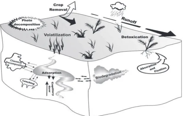
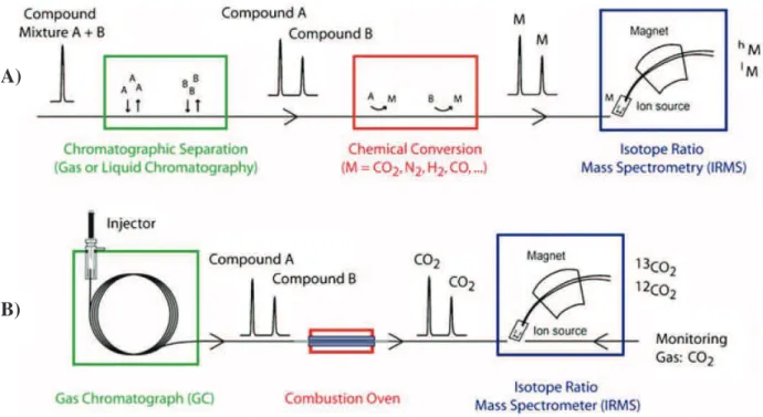
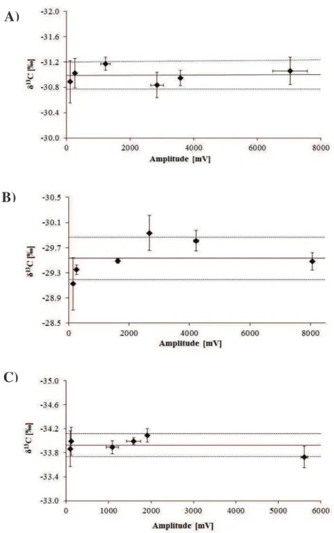
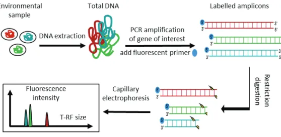
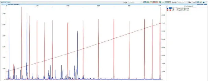
Figure I-1. Processes driving the fate of pesticides in the environment. ... 5 Figure I-4: Chloroacetanilide herbicides and their degradation products ... 14 Figure I-5: Example Rayleigh plots of carbon and nitrogen isotope fractionation during the oxidation of nitrobenzene by Comamonas sp. strain JS765 ... 21 Figure I-6: Biogeochemical cycles of nitrogen, carbon and sulphur in wetlands ... 30 Figure I-7: Processes of pesticide removal in wetlands ... 31 Figure I-8: Graphical outline representing Chapters III and IV of this PhD thesis. ... 40 Figure II-1. The principle (A) and instrumentation (B) of compound-specific isotope analysis by gas chromatography combustion isotope ratio mass spectrometry ... 43 Figure II-3. Linearity tests for (A) metolachlor, (B) acetochlor and (C) alachlor.. ... 48 Figure II-4: Pathway of acetochlor degradation by Sphingobium DC2. ... 52 Figure II-5: Main steps of the T-RFLP procedure ... 62 Figure II-6. Example T-RFLP electropherogram as visualised using PeakScanner software showing sample peaks (blue) and size marker peaks (red). ... 66 Figure III-1. Picture (A) and schematic representation (B) of the vertical flow lab-scale wetlands ... 76 Figure III-2. Carbon isotope signatures of metolachlor, acetochlor and alachlor in lab-scale wetlands ... 82 Figure III-3. Relative concentrations (Cx/Cin = concentration at point (x) divided by inlet

concentration) for metolachlor (triangles), alachlor (squares) and acetochlor (circles) and corresponding average oxygen concentrations at different depths in lab-scale wetlands ... 90 Figure III-4. Linearized Rayleigh plots for alachlor A) and acetochlor B). ... 92 Figure III-5. Concentrations of terminal electron acceptors (TEAs) oxygen (black circles), nitrate (grey triangles) and sulphate (white squares) in column wetlands.. ... 102 Figure III-6. Mean enantiomer fraction (± SD) of metolachlor along the flow path for the period between day 0 and day 112. ... 104 Figure III-7. 2D-NMDS ordination of T-RFLP bacterial profiles (A) and a posteriori fitting of environmental parameters (B). ... 106 Figure III-8. 2D-NMDS ordination of A) pyrosequencing (97% sequence identity) and B) corresponding T-RFLP bacterial community profiles of sequenced lab-scale wetland samples.. ... 108

(30)

XXVIII lab-scale wetland outlets on day 0 and day 70, and in the anoxic zone (at 45 cm from inlets) of wetlands contaminated with metolachlor (Met), acetochlor (Acet) and alachlor (Ala) on day 70... 110 Figure III-10. Chromatogram of metolachlor diastereisomers obtained with chiral GC-MS analysis. ... 123 Figure III-11. Reddish-brown ferric iron oxide precipitates along Phragmites australis root periphery in a lab-scale wetland. ... 123 Figure III-12. Load removal of metolachlor, alachlor and acetochlor between two sampling campaigns from day 0 to day 112. ... 124 Figure III-13. 2D-NMDS ordination of T-RFLP bacterial community profiles. ... 125 Figure III-14. Rarefaction curves for bacterial OTUs. ... 126 Figure IV-1. Schematic representation of (A) subsurface-flow constructed wetlands investigated in this study (B) hydraulic operation and contamination for the two wetlands. 133 Figure IV-2. Biogeochemical processes and metolachlor degradation in the two wetlands. 139 Figure IV-3. 2D-NMDS ordination of bacterial community profiles based on (A) T-RFLP and (B) pyrosequencing of the V1-V3 hypervariable region of the 16S rRNA gene in total DNA from wetland water and rhizosphere samples. ... 142 Figure IV-4. Relative abundance [%] of dominant bacterial classes (80% sequence identity threshold) in the wetland water samples on different sampling days (days 0, 35 and 56) and in the rhizosphere samples. ... 146 Figure IV-5. 2D-NMDS ordination of bacterial profiles based on T-RFLP of the 16S rRNA gene from wetland inlet, outlet and piezometer samples. ... 157 Figure IV-6. Rarefaction curves for bacterial sequences of the V1-V3 hypervariable region of the 16S rRNA gene with OTUs defined at 97% sequence identity.. ... 158 Figure V-1. Proposed approaches for improving assessments of chloroacetanilide-contaminated wetlands ... 162

(31)

XXIX

Liste de figures

Figure I-1. Processus régissant le devenir des pesticides dans l'environnement ... 5 Figure I-4: Les herbicides chloroacétanilides et leurs produits de dégradation ... 14 Figure I-5: Exemple de fractionnement isotopique du carbone et de l'azote au cours de l'oxydation du nitrobenzène par la souche Comamonas sp. JS765 ... 21 Figure I-6: Cycles biogéochimiques de l'azote, du carbone et du soufre dans les zones humides ... 30 Figure I-7: Processus de l'élimination des pesticides dans les zones humides ... 31 Figure I-8: Aperçu graphique pour les chapitres III et IV du manuscrit de thèse. ... 40 Figure II-1. Principe (A) et instrumentation (B) @-"/51(1/8B-"*B.).<*+,-"0.6<.B'-spécifique par chromatographie gazeuse > combustion-spectrométrie de masse de rapport isotopique .. 43 Figure II-3. Test de linearité pour (A) le métolachlore, (B) l'acétochlore et (C) l'alachlore.. . 48 Figure II-4: H.*-"@-"@'921@1)*.("@-"/510').0=/.2-"<12 Sphingobium sp. DC2. ... 52 Figure II-5: Principales étapes de la T-RFLP ... 62 Figure II-6. Ex-6</-" @5'/-0)2.<='rogramme de T-RFLP 7*B,1/*B'" K" /51*@-" @," /.9*0*-/" PeakScanner ... 66 Figure III-1. Photographie (A) et représentation schématique (B) des zones humides en colonnes ... 76 Figure III-2. Signatures isotopiques du carbone du métolachlore, de l'acétochlore et de l'alachlore dans les zones humides en colonnes ... 82 Figure III-3. Concentrations relatives (Cx/Cin = concentration au point (x) divisée par la

concentration d'entrée) pour le métolachlore (triangles), l'alachlore (carrés) et l'acétochlore (cercles) et les concentrations moyennes d'oxygène à différentes profondeurs dans les zones humides en colonnes ... 90 Figure III-4. Graphique de Rayleigh pour /5alachlore A) et l'acétochlore B). ... 92 Figure III-iC" Q.(0-()21)*.(B" @5100-<)-,2B" terminaux @5'/-0)2.(s: oxygène (cercles noirs), nitrate (triangles gris) et sulfate (carrés blancs) dans les zones humides en colonnes.. ... 102 Figure III-6. Fraction énantiomérique moyenne (± écart-type) du métolachlore entre les jours 0 et 112.. ... 104 Figure III-7.Représentation 2D-NMDS des profils bactériens T-RFLP (A) et des paramètres environnementaux (B). ... 106

(32)

XXX (97% d'identité de séquence) et B) la T-RFLP des échantillons des zones humides en colonnes. ... 108 Figure III-9. L'abondance relative [%] des classes bactériennes (seuil d'identité de séquence = 80%) dans les sorties des zones humides en colonnes au jour 0 et au jour 70, ainsi que dans la zone anoxique (à 45 cm de /5-()2'-) des zones humides contaminées avec le métolachlore (Met), /5acétochlore (Acet) et l'alachlore (Ala) au jour 70 et au jour 110 ... 110 Figure III-10. Chromatogramme des diastéreoisomères du métolachlore obtenu en utilisant /51(1/8B-"&Q-MS chirale... 123 Figure III-11. Précipité brun rougeâtre @-"/5oxyde de fer(II) le long des racines de Phragmites australis dans une zone humide en colonne. ... 123 Figure III-12. Réduction de masse du métolac=/.2-3" @-" /51/10=/.2-" -)" @-" /510').0=/.2e entre deux campagnes d'échantillonnage entre le jour 0 et le jour 112. ... 124 Figure III-13. Représentation 2D-NMDS de profils T-RFLP de communautés bacteriennes. ... 125 Figure III-14. Courbes de raréfaction des OTUs bactériennes ... 126 Figure IV-1. Représentation schématique des zones humides artificielles aux flux aquatique sousterrain examinés dans cette étude. (A) fonctionnement hydraulique et (B) contamination pour les deux zones humides ... 133 Figure IV-2. Processus biogéochimiques et dégradation du métolachlore dans les deux zones humides ... 139 Figure IV-3. Représentation 2D-NMDS des profils de communautés bactériennes basés sur (A) la T-RFLP et (B) le pyroséquençage de la région hypervariable V1-V3 du gène ARNr 16S de l'eau des zones humides et des échantillons de la rhizosphère ... 142 Figure IV-4. . L'abondance relative [%] des classes bactériennes dominantes (seuil d'identité de séquence = 80%) dans les échantillons d'eau des zones humides pour les différents jours d'échantillonnage (jours 0, 35 et 56) et dans les échantillons de la rhizosphère. ... 146 Figure IV-5. Représentation 2D-NMDS des profils bactériens basés sur T-RFLP du gène ARNr 16S à l'entrée des zones humides, à la sortie et aux échantillons des piézométres. ... 157 Figure IV-6. Courbes de raréfaction pour les séquences bactériennes des régions hypervariables V1-V3 du gène ARNr 16S avec les OTUs définis à ,("B-,*/"@5*@-()*)'"@-"B'+,-(0-"@-"lmn. ... 158 Figure V-1. Approches proposées pour l'amélioration de l'évaluation des zones humides contaminées par les chloroacétanilides ... 162

(33)

XXXI

List of tables

Table I-3. Approaches of evaluation of pesticide degradation ... 16 Table II-2. Target functional genes and their corresponding primer pairs. ... 56 Table II-3. Detection of target functional genes in constructed wetland samples ... 60 Table II-4. Comparison of the two T-RFLP data treatment methods. ... 67 Table III-1. Bulk enrichment factors and AKIE values calculated for alachlor and acetochlor for sampling campaigns at days 42, 70 and 98 and for data from the three campaigns combined ... 84 Table III-2. Average values (mean ± standard deviation) for hydrochemical parameters of inlets and outlets of lab-scale wetlands from day 0 to day 98. ... 88 Table III-3. Average mass removal [%] of metolachlor, alachlor and acetochlor between inlets and outlets of lab-scale wetlands between day 28 and 98, and during the three periods of isotope investigation. ... 89 Table III-cC" $-1(" 1(@" B)1(@12@" @-7*1)*.(B" .:" B)1A/-" 012A.(" *B.).<-" [h13_{C) triplicate}

measurements for two weeks old inlets (two weeks inlet), freshly spiked inlets (fresh inlet) and outlets at days 42, 70 and 98. ... 91 Table III-5. Physicochemical properties of the filling materials used for the lab-scale wetlands. ... 121 Table III-7. Diversity and richness indices calculated for lab-scale wetland water samples by T-RFLP and by 454 pyrosequencing (OTUs at 97% sequence identity) for days 0, 14, 70 and 98... 127 Table IV-1. Inlet water volumes and injected S-metolachlor concentrations and masses in both studied wetlands. ... 154 Table IV-2. Hydrochemical parameters of water samples from the inlet (tap water), outlet and piezometers of the continuous and the batch wetlands. ... 155 Table IV-3. Daughter ions and transition SRM used for GC-MS/MS quantification of S-metolachlor and LC-MS/MS quantification of its ionic degradation products ESA and OXA. ... 156 Table IV-4. ;=1((.("@*7-2B*)8"*(@-T"Z5"1(@"(,6A-2".:"FN#B calculated for wetland samples by T-RFLP (T-RFs) and by 454 pyrosequencing (97% sequence identity), and for rhizosphere samples. ... 159

(34)

XXXII

Liste des tableaux

Table I-3. Approches de l'évaluation de la dégradation des pesticides... 16 Table II-2. Les gènes fonctionnels ciblés et leurs correspondants amorces. ... 56 Table II-3. Détection de gènes fonctionnels dans 60 échantillons de zones humides artificielles ... 60 Table II-4. Comparaison de deux méthodes de traitement des données T-RFLP ... 67 Table III-1. Facteurs d'enrichissement et valeurs AKIE calculés pour /5alachlore et /5acétochlore pour les campagnes d'échantillonnage à jour 42, 70 et 98 et pour les données combinées des trois campagnes ... 84 Table III-2. Les valeurs moyennes (moyenne ± écart-type) des paramètres hydrochimiques des entrées et sorties des zones humides K"/5échelle du laboratoire du jour 0 au jour 98 ... 88 Table III-3. Réduction de masse moyenne [%] du métolac=/.2-3" @-" /51/10=/.2-" -)" @-" /510').0=/.2e entre les entrées et les sorties des zones humides en colonnes entre le jour 28 et 98, ainsi que pendant les trois périodes d'analyse des isotopes. ... 89 Table III-4. Moyennes et écarts-types des mesures isotopiques en triplicat du carbone stable [h13C) pour les entrées datant de deux semaines, les entrées fraîchement préparées et les sorties aux jours 42, 70 et 98 ... 91 Table III-5. Des propriétés physico-chimiques des matériaux de remplissage utilisés pour les zones humides en colonnes. ... 121 Table III-7. Indices de diversité et de richesse calculés pour les échantillons d'eau des zones humides en colonnes par T-RFLP et par pyroséquençage 454 (OTU à 97% d'identité de séquence) pour les jours 0, 14, 70 et 98 ... 127 Table IV-1. Les volumes d'eau @5-()2'-3" /-B" concentrations et masses de S-métolachlore injectés dans les deux zones humides étudiées. ... 154 Table IV-2. Paramètres hydrochimiques d'eau d'entrée (eau du robinet), de sortie et des piézomètres des zones humides en flux continu et en discontinu ... 155 Table IV-3. Ions fils et transition SRM utilisées pour la quantification GC-MS/MS du S-métolachlore et la quantification LC-MS/MS de produits de dégradation ionique ESA et OXA. ... 156 Table IV-4. Indices de diversité Shannon H et nombre d'OTUs pour les échantillons @5-1,"des zones humides et pour les échantillons de rhizosphère par T-RFLP (T-RFs) et par pyroséquençage 454 (identité de séquence de 97%) ... 159

(35)

(36)

1

Chapter I

Introduction

This Chapter provides background information about the main subjects of interest of this PhD work, namely reactive transport of pesticides in wetland systems. First, the relevance of studying pesticide contamination and degradation in the environment, focusing on our target family: the chloroacetanilide herbicides, is reviewed. Then, methods for monitoring pesticide degradation in the environment are presented and the advantages and limitations of each tool are highlighted. The main biogeochemical characteristics and functioning of wetlands, our 0=.B-(" o6.@-/5" -0.Bystems for studying pesticide (bio)degradation, are discussed. We then discuss wetland biogeochemical and pesticide degrading processes as well as the impact of pesticides on wetland bacterial communities. Finally, the focus and objectives of this PhD thesis are presented.

(37)

2

1. Pesticides

Use, ecological and human health impact

Since the introduction of the first synthetic organic pesticide DDT (dichlorodiphenyltrichloroethane) in the 1940s, pesticides have been increasingly used to increase agricultural crop yields. The number of pesticide molecules developed has been steadily rising along with the global pesticide production. Currently, there are more than 536 and 1,055 different registered pesticides molecules in the EU and the USA (Sierka, 2013; EU, 2014). An estimated 2.4 million tons of pesticide active ingredient is applied worldwide every year, 90% of which is applied on agricultural fields. Herbicides comprise the largest portion of the pesticides used (39%), followed by insecticides (18%), and fungicides (10%) (EPA, 2011). Due to this extensive worldwide use, pesticides became a major source of diffuse environmental pollution (Mostafalou and Abdollahi, 2013). Nine out of the twelve dangerous persistent organic pollutants of the initial list identified by the Stockholm Convention in 2004 were pesticides (Patterson et al., 2009). Numerous persistent pesticides were still detected in environment several years after the ban of their use. Organochlorine pesticides including <3<p-dichlorodiphenyltrichloroethane (DDT), hexachlorobenzene, endoslfan, and q-hexachlorocyclohexane could still be detected in soil, water, fish and even in human milk decades after the ban of their use (Kurt-Karakus et al., 2006; Darko et al., 2008; Mueller et al., 2008). Another example is atrazine that remained the most abundant pesticide in groundwater in Germany almost two decades after its ban (Jablonowski et al., 2011). A recent study revealed the extent of pesticide contamination of freshwater ecosystems in the EU by monitoring pesticide concentrations in 4,001 sites distributed in 91 European rivers. Pesticides exceeded the acute risk threshold for fish, invertebrates and algae in 81%, 87%, and 96% of the tested samples, respectively (Malaj et al., 2014). Pesticides were also found to be among the most relevant and important contaminants of ground water in Europe. The insecticide N,N-Diethyl-meta-toluamide (DEET) was detected in 84% of groundwater samples while other pesticides such as atrazine, diuron, simazine and isoproturon were detected in 20 to 56% of the samples (Loos et al., 2010). The above mentioned examples give a glimpse of the extent of the pesticide contamination in different environmental compartments.

The widespread pesticide contamination comes with consequences on the environment and human health. N=-"/1(@612M"A..M" ;*/-()";<2*(9!"A8"%10=-/"Q12B.("[blr`^"?1B")=-":*2B)")."

(38)

3 expose potential damage to the environment and human health caused by pesticides, and thereby drew public attention to the issue. Numerous scientific studies showed the detrimental impact of pesticide exposure on humans, and a wide diversity of flora and fauna (Dawson et al., 2010; Kohler and Triebskorn, 2013). For example, long-term pesticide exposure has been linked to increased incidence of prostate cancers by hindering DNA repair mechanisms in pesticide applicators and pesticide manufacturing workers (Barry et al., 2012). Another study reported the link between residential pesticide use and increased risk of melanoma cancers

(Fortes et al., 2007). Similarly, higher serum levels of DDE

(dichlorodiphenyldichloroethylene), a metabolite of the pesticide DDT, correlated with an increased risk for Alzheimer disease (Richardson et al., 2014) while an increased risk for G12M*(B.(5B" @*B-1B-" 16.(9" .)=-2" (-,2.@-9-(-21)*7-" @*B-1B-B" ?1B" /*(M-@" ?*)=" 0=2.(*03" (.(-occupational exposure to pesticides (Parron et al., 2011). Numerous pesticides have raised concerns due to their endocrine disruptive properties including: insecticides such as chlorpyrifos, chlordane, parathion, lindane, and malathion; herbicides such as diuron, prodiamine, thiazopyr, trifluralin; and fungicides such as vinclozolin, phenylphenol, and carbendazim (Murray et al., 2010). Pesticides were also associated with toxicity to aquatic organisms (Groner and Relyea, 2011), animals (Amaral et al., 2012), and plants (Andresen et al., 2012). Recently, the role of neonicotinoid insecticides in the decline of populations of pollinator bees has been demonstrated (Whitehorn et al., 2012), where imidacloprid-contaminated bumble bee colonies were found to be significantly smaller in size and produced less queens than non-contaminated colonies. Given their crucial role as pollinators, the decline of bee populations threatens crop production potentially on a global scale. In addition to their toxic effects on humans, animals, insects and aquatic organisms, pesticides also impact microorganisms in soil and water ecosystems (Imfeld and Vuilleumier, 2012), subsequently influencing nutrient and biogeochemical cycles (Kinney et al., 2005; Schafer et al., 2012). As a result of the numerous deleterious effects of pesticides on the environment and human health, the understanding of the behaviour and fate of pesticides in the environment has become a subject of main interest for the scientific community, reflecting the societal concerns.

(39)

4 Transport and attenuation in the environment

Pesticide contamination is mainly diffuse and caused by losses of intentionally applied pesticides in agricultural fields, but can also be caused by high-level point source pesticide release (e.g. accidental spills) (Vega et al., 2007). Most of the load of pesticides applied in agriculture reaches non-target compartments causing contamination of soil, water and air. During application, 1 to 75% of pesticides can be transported via drift to non-target areas (Lefrancq et al., 2013; Barbash, 2014). After application, 50 - 60% of the pesticides are typically transported to the atmosphere via volatilisation (Grégoire et al., 2009). The volatilised loads of pesticides can then contaminate soil and water bodies through water deposition (rainfall), or dry deposition (gaseous and solid particles precipitation). Once on the soil, a part of the pesticides can be attenuated by destructive processes which are mainly mediated by soil micro-organisms (Fenner et al., 2013). The non-degraded fraction of pesticides can, however, be mobilised by rain and transported through runoff to downstream water bodies, or leach through the soil until reaching groundwater ecosystems (Botta et al., 2012; Farlin et al., 2013). An estimated range of 1-10% of pesticide load applied is found in downstream surface water bodies that include streams, rivers and lakes in areas surrounding agricultural catchments (Schulz, 2004).

The contribution of the different routes of transport and degradation on the fate of pesticides in the environment depends on a number of extrinsic factor (e.g. climate conditions, agricultural landscape and practices, additives in pesticide formulations), and intrinsic factors specific to each pesticide molecule (e.g. volatility, hydrophobicity, solubility). For instance, highly volatile pesticides are mostly influenced by spray drift and volatilisation. Pesticides with relatively high organic carbon water coefficients (Koc s"cba^"have a strong tendency to sorb to

organic material in soil and sediment and more likely to persist for long periods of time with low perspective of degradation (De Wilde et al., 2009), and are mainly transported by soil erosion or by transport on soil particles (Maillard et al., 2011). On the contrary, polar pesticides with higher water solubility are more likely to be transported via rainfall-runoff and leach to receptor water bodies. Their high bioavailability increases their risk to aquatic and soil organisms as well as their potential for biodegradation (Yu et al., 2006). Likewise, pesticide degradation products which are typically more polar than their precursors are thus more prone to mobilisation (Escher and Fenner, 2011). Their high mobility makes degradation products

(40)

5 relevant contaminants of surface and ground water (Huntscha et al., 2008). Pesticide degradation products are of particular relevance if they are formed in large amounts and/or are persistent, if they are more mobile than the parent compounds, and/or if they are highly toxic (Escher and Fenner, 2011). Unlike physical attenuation processes (e.g. sorption, volatilisation), degradation processes are the only true means of removal of pesticide contamination in the environment. Generally, microbial degradation is considered to be the dominant process of pesticide degradation (Fenner et al., 2013). Yet, abiotic degradation processes can also be of relevance under certain circumstances. For example, photodegradation contributed considerably to the degradation of several pesticides in surface prairie lakes water (Zeng and Arnold, 2013)C"F)=-2"o@12M5"1A*.)*0"@-921@1)*.("<2.0-BB-B".00,2"1)"7-28"/.?"21)-B"1(@")=-2-:.2-" usually of little importance. However, this trend can be reversed under specific conditions, e.g. in environments with high pH (e.g. hydrolysis 1)"<Z""s"t (Zhang et al., 2013b)) , or in the presence of suitable catalysts (e.g. chloroacetanilide herbicides degradation in sulphidic environments (Zeng et al., 2011)). The interplay between the different transport and degradation processes determine the fate of pesticides in the environment and consequently the levels of exposure to pesticide contamination in downstream ecosystems (Rice et al., 2007).

Figure I-1. Processes driving the fate of pesticides in the environment (Andreu and Picó,

(41)

6 Several factors add to the severity of the issue of pesticide contamination. One of these factors is the increasing proportion of chiral pesticides with the introduction of pesticides with more complex molecular structures. More than 30% of currently used pesticides are chiral compounds, including pyrethoids, organophosphate insecticides, imidazolinone and metolachlor (Liu et al., 2005). Chiral molecules contain at least one stereo-centre that is often an asymmetrically substituted carbon atom giving rise to two or more enantiomers which are non-superimposable mirror images of each other. Figure I-2 shows stereoisomers of the chiral pesticide metolachlor. Enantiomers of chiral pesticides have identical physicochemical properties (solubility, vapour pressures, and partition coefficients among air, water and octanol) and transport processes (advection, deposition, volatilisation, diffusion) and abiotic reactions (photolysis, hydrolysis) will not change enantiomer proportions (Bidleman et al., 2013). On the contrary, enantiomers may differ in their binding to stereo-sensitive biological receptors and naturally occurring chiral biomolecules because of their different molecular configurations (Hegeman and Laane, 2002).

Accordingly, enantiomers may exhibit different biological activities, toxicities, and degradation processes in organisms and the environment (Ye et al., 2010). In many of the chiral pesticides that are commercialised as racemates, only one of the enantiomers possesses the target activity (e.g. herbicidal) while the other enantiomer is present in the commercial formulation as a by-product of the pesticide synthesis process (Diao et al., 2010; Ye et al., 2013). Enantiomers of pesticides need therefore to be assessed separately for toxicity, and environmental fate. Likewise, additives (e.g. surfactants) are concomitantly released in the environment with pesticides and represent new potential contaminants with different environmental behaviour and toxicity, and therefore need to be taken into account for the approval of pesticide commercial formulations (Schenker et al., 2007; Oliver-Rodríguez et al., 2013). Pesticide degradation products are also increasingly being considered in pesticide risk assessments, in particular if they prove to be more toxic, more persistent or more mobile than their parent compounds (Escher and Fenner, 2011). Finally, the emerging nanopesticide technology present a new challenge for pesticide risk assessments (Kah and Hofmann, 2014). Nanopesticides refer to an emerging class of pesticides in which nanotechnology (e.g., use of materials that have a physical form with at least one size dimension in the range of 1>100 nm) is employed to enhance the efficacy or reduce the environmental footprint of a pesticide active

(42)

7 ingredient. For example, the encapsulation of pesticide active ingredient in nanocapsules for controlled release or targeted delivery of pesticide active ingredient. New risk assessment procedures will be needed to take into consideration the impact of the use of such nanoformulations on the activity and toxicity of known pesticide active ingredients (Kookana et al., 2014).

Figure I-2. Stereoisomers of metolachlor. Chiral centres are denoted by asterisks. Also indicated are the diastereomeric and enantiomeric relationships between isomers.

(Muller et al., 2001).

In spite of decades-long use of pesticides, predictions of pesticide fate in the environment remain elusive. It is therefore important to understand the interplay of processes that control fate of pesticides in the environment; transport routes (e.g. via aerial deposition, erosion, runoff) phase transfer processes (e.g. sorption and volatilisation) and degradation processes. Pesticide degradation is of particular importance since it is the only process that effectively eliminates pesticide molecules from the environment. The type and rate of degradation processes of pesticides in a given environment is determined by intrinsic factors to the pesticide molecule (e.g. molecular structure, hydrophobicity) and environmental factors (e.g. redox, pH, temperature) (Knabel et al., 2012; Fenner et al., 2013b). Traditionally studies of pesticide degradation in the environment mainly depend on concentration analysis and mass balance approaches to demonstrate pesticide attenuation, but these approaches provide little information on in situ removal processes. Consequently, new approaches are needed to i) demonstrate the occurrence of in situ pesticide degradation, ii) identify conditions under which

(43)

8 degradation takes place, and iii) when possible, quantify the extent of degradation. Methods for assessing pesticide degradation in the environment are discussed in section 3. In the following section we focus on the properties and environmental fate the target family of herbicides of this PhD thesis work: chloroacetanilide herbicides.

2. Chloroacetanilide herbicides

Properties and use

Chloroacetanilide herbicides form a sub-group of amide herbicides. They share a chloroacetanilide core moiety and mainly differ in their alkoxyalkyl group attached to the nitrogen atom of the amide group, and the methyl or ethyl benzene ring substituents (Figure I-3). They are widely used to control annual grasses and broad-leaved weeds on a variety of crops including maize, sugar beet and sunflower (Zhang et al., 2011). Chloroacetanilides act by inhibiting the elongation of C16 and C18 to C20 fatty acids to very long chain fatty acids in susceptible weeds, leading to imbalance in fatty acid composition and thus to the weakening of cell membranes (Gotz and Boger, 2004). Chloroacetanilides include metolachlor, acetochlor, alachlor, propachlor and butachlor among others. Alachlor was widely used in the 1990s until the EU banned its use in 2006 due to concerns regarding elevated human exposure due to extensive ground water contamination and potential carcinogenicity (Heydens et al., 1999). Alachlor was largely replaced by acetochlor that was also banned in the EU in 2012. The ban came after evidence of the high human exposure of acetochlor and its metabolite t-norchloroacetochlor, and the high risk of acetochlor to aquatic organisms and birds (European food safety authority, 2011). Metolachlor is a chiral molecule containing two stereogenic centres; an asymmetrically substituted carbon and a chiral axis giving rise to four stereoisomers; two pairs of enantiomers and two pairs of diastereoisomers (Figure I-2). Metolachlor was first introduced in 1979 as a racemic mixture, containing equal ratios of the two enantiomers, which was later replaced in 1990s by a formulation enriched with the herbicidally active S-enantiomer (S-metolachlor) (Ma et al., 2006). S-metolachlor and acetochlor were the fourth and fifth most commonly used pesticides in the USA between 2001 and 2007 (EPA, 2011).

(44)

9

Figure I-3. Molecular structure of the chloroacetanilide herbicides metolachlor, acetochlor and alachlor. The chloroacetanilide common moiety is highlighted in pale blue.

S-metolachlor is currently the most widely used chloroacetanilide herbicide despite its higher persistence and recalcitrance to degradation in soil and water compared to other chloroacetanilides, as was demonstrated in several studies (Graham et al., 1999; Zhang et al., 2011a). In addition to differences in herbicidal activity, metolachlor enantiomers exhibit different toxicities towards earthworms (Xu et al., 2010), aquatic organisms (Liu and Xiong, 2009), and rice and maize roots (Liu et al., 2012a). Preferential degradation of the S-enantiomer was observed in soil and sludge (Muller et al., 2001; Ma et al., 2006), whereas another study reported the absence of enantioselective degradation of metolachlor in soil (Klein et al., 2006). The environmental conditions under which enantiomer-specific degradation of metolachlor is occurs, the microbial populations, pathways and enzymes involved in this enantioselective degradation process remain unknown.

Environmental fate of chloroacetanilide herbicides

Chloroacetanilide herbicides are pre-emergence herbicides (i.e. applied before the development of a vegetal cover) to inhibit seed germination which, along with their relatively high water solubility, makes them prone to mobilisation by runoff and to contaminate aquatic ecosystems (Reid et al., 2000). Indeed, chloroacetanilides and their degradation products are frequently detected in ground and surface water which raises concerns about their environmental and human health impacts (Baran and Gourcy, 2013b; Postigo and Barcelo, 2014). Chloroacetanilides are characterised by low volatility (Henry constants > 10-3_{Pa m}3