The Current Feedback to the Atmosphere : Implications for the Ocean Dynamics, Air-Sea interactions, and How to Best Force an Ocean Model

(1)

HAL Id: tel-02084330

https://hal.archives-ouvertes.fr/tel-02084330v2

Submitted on 2 Oct 2020

HAL is a multi-disciplinary open access archive for the deposit and dissemination of sci-entific research documents, whether they are pub-lished or not. The documents may come from teaching and research institutions in France or abroad, or from public or private research centers.

L’archive ouverte pluridisciplinaire HAL, est destinée au dépôt et à la diffusion de documents scientifiques de niveau recherche, publiés ou non, émanant des établissements d’enseignement et de recherche français ou étrangers, des laboratoires publics ou privés.

The Current Feedback to the Atmosphere : Implications

for the Ocean Dynamics, Air-Sea interactions, and How

to Best Force an Ocean Model

Lionel Renault

To cite this version:

Lionel Renault. The Current Feedback to the Atmosphere : Implications for the Ocean Dynamics, Air-Sea interactions, and How to Best Force an Ocean Model. Ocean, Atmosphere. Université Paul Sabatier - Toulouse 3, 2018. �tel-02084330v2�

(2)

THÈSE P

RÉSENTÉE POUR OBTENIR

L’HABILITATION À DIRIGER DES

RECHERCHES

SPÉCIALITÉ: OCÉANOGRAPHIEPHYSIQUE

The Current Feedback to the

Atmosphere : Implications for the Ocean

Dynamics, Air-Sea interactions, and How

to Best Force an Ocean Model

October 12, 2018

Author

Lionel RENAULT

Jury

Eric CHASSIGNET: Rapporteur

Hervé GIORDANI: Examinateur

Patrick MARCHESIELLO: Président

Sebastien MASSON: Examinateur Sabrina SPEICH: Rapporteure Anne-Marie TREGUIER: Rapporteure

(3)

Table des matières

Introduction 6

1 A Description of the Data, Experiments and Methods 11

1.1 Data . . . 13

1.2 Current Feedback in a Coupled Model . . . 13

1.3 Numerical Experiments . . . 14

1.4 A Simplified Kinetic Energy Budget . . . 24

1.5 A Full KE budget . . . 26

1.6 Spectral Flux of Surface Ocean Geostrophic Kinetic Energy . . . 27

1.7 Coupling Coefficients . . . 27

1.8 Miscellaneous . . . 29

2 A Direct Control of the Oceanic Circulation, from the Large Scale to the Subme-soscale 32 2.1 A Large Scale Effect: A Slow Down of the Gyre . . . 33

2.2 At the Mesoscale: An "Eddy Killer" . . . 38

2.3 At the Submesoscale: A Catalizer but Still a Killer, the case of the California Current System . . . 48

2.4 Conclusion of the Chapter . . . 58

3 Control of the Western Boundary Currents by the Current Feedback 61 3.1 The Case of the Gulf Stream . . . 63

3.2 The Case of the Agulhas Current . . . 65

3.3 Reduction of the Eddy-Mean Flow Interactions . . . 71

3.4 Conclusion of the Chapter . . . 74

4 On the Atmospheric Response to the Current Feedback 77 4.1 Coupling Coefficient between Current and Stress . . . 78

(4)

4.2 Coupling Coefficient between Current and Wind . . . 85 4.3 Indirect Effect on the Precipitation over the Agulhas Current . . . 88 4.4 Conclusion of the Chapter . . . 91

5 Disentangling the Mesoscale Thermal and Current Feedbacks 92

5.1 Disentangling The Current Feedback . . . 95 5.2 Disentangling The Thermal Feedback . . . 98 5.3 Conclusion of the Chapter . . . 105

6 Perspectives 108

6.1 Toward a New Paradigm: Recipes How to Best Force an Ocean Model . . . 109 6.2 On the Biogeochemical Response . . . 117 6.3 Control of the Precipitation by Mesoscale Air-Sea Interactions . . . 118 6.4 A Missing Piece of the Puzzle: the Wave Feedbacks to the Atmosphere and

the Ocean . . . 119

7 Conclusion 124

8 Projects and Mentoring 127

8.1 Implication in Research Project . . . 128 8.2 Mentoring and Research Team . . . 132 8.3 Referring activities and outreach . . . 134

9 Publications and Divulgation 136

List of Figures 142

List of Tables 155

(5)

Résumé

Les interactions entre l’océan et l’atmosphère influencent largement le cli-mat de la Terre ainsi que les écosystèmes à l’échelle des bassins océaniques. Les principaux modes de variabilité climatique (ex : Oscillation Madden-Julian, El Niño, Oscillation Nord-Atlantique) sont des modes couplés entre ces deux milieux. Les écosystèmes ont une forte réponse à ces variations à travers l’in-fluence physique des vents, de la lumière et de la température, sur le réser-voir de nutriments et donc sur la production primaire et la chaine trophique. Les biais en température de surface de la mer dans les modèles globaux ont mis en lumière les limites d’une approche globale et ont ainsi fait surgir une nouvelle ligne de recherche basée sur une approche régionale des interactions entre l’océan et atmosphère permettant de mieux comprendre et prévoir la variabilité dans des régions clefs de l’océan. Il a donc récemment été montré qu’à l’échelle régionale, les interactions fines échelles entre l’océan et l’atmo-sphère peuvent aussi grandement moduler la variabilité et l’état moyen de l’océan et de l’écosystème associé. Le changement climatique a et aura une influence sur les interactions entre l’océan et l’atmosphère et donc sur l’éco-système aussi bien d’un point de vue global que régional. Comprendre quels sont les processus clés qui gouvernent l’état moyen et la variabilité physique et biogéochimique, et quel est et sera l’impact du changement climatique sur ces processus, s’avère donc primordial. C’est ce qui a motivé ma recherche dans ce domaine et a orienté mon parcours. Comme je vais le présenter dans ce manuscrit, ma ligne de recherche part du postulat suivant (que j’étaye en-suite par certains de mes travaux) : afin de comprendre l’évolution de l’océan, et ainsi l’impact du changement climatique, il est nécessaire d’avoir une ap-proche intégrée basée sur la compréhension des phénomènes physiques. Je me suis donc toujours attaché à caractériser les fines échelles océaniques et at-mosphériques à partir des observations, puis à les modéliser et analyser leurs interactions et impacts sur la variabilité et l’état moyen de l’océan et, quelques fois, de l’écosystème. Ma démarche s’est tout d’abord appliquée principale-ment aux Systèmes d’Upwelling de Bord-Est, mais, de par mes expériences professionnelles en Espagne et aux Etats-Unis, ainsi que les projets, étudiants, et postdocs que j’ai supervisés, j’ai pu l’étendre sur de diverses régions, allant de la Mer Méditérannée aux courants de Bord-Ouest.

(6)

En particulier, j’ai rédigé plusieurs études sur l’origine et les conséquences de la diminution du vent à l’approche du continent (le «drop-off» du vent) dans les Courants de Bord-Est. J’ai démontré son importance dans la détermination de la circulation moyenne et mésoéchelle mais aussi de la production primaire nette. Cependant, dans ce manuscrit, j’ai décidé de me concentrer sur un autre aspect de ma recherche qui a été très inspirant pour moi, et qui, comme discuté dans ce qui suit, pourrait (et je pense devrait) conduire à un changement de pa-radigme sur la façon de forcer un modèle océanique : l’influence des courants océaniques de surface sur le vent et la réponse océanique associée. Je présente aussi à la fin de ce manuscrit une réfléxion sur ma carrière ainsi qu’une pré-sentation des principaux projets de recherche et des étudiants supervisés.

(7)

Abstract

The Ocean-Atmosphere interactions have a large influence on the climate and on the ecosystems at the basin scale. The main climatic modes of vari-ability (e.g., El Niño, NAO, ...) are coupled modes between the Ocean and the Atmosphere. The ecosystems have a strong response to those variations through the influence of the wind, the light, and the temperature on the nu-trient stock and, thus, on the primary production and the oxygen concentra-tion. Systematic biases in sea surface temperature in global models have high-lighted the limitations of studies based on the global models and have, thus, spurred the investigation of the Ocean-Atmosphere interactions based on the regional modeling approach. In the past few years,it has been demonstrated that the regional Ocean-Atmosphere interactions can strongly modulate the variability and the mean physical and biogeochemical state of the ocean. My line of research starts from the following postulate: in order to understand the evolution of the ocean and ecosystems and thus the impact of climate change, it is necessary to have an integrated approach based on the understanding of physical phenomena and their interactions with the ecosystem at relevant spa-tial and temporal scales. I have always focused on characterizing fine oceanic and atmospheric scales from observations and then modeling them and ana-lyzing their interactions and impacts on the ocean variability and mean state. I applied my approach over different regions of the world, including East-ern and WestEast-ern Boundary Current Systems, the Mediterranean Sea, and also more recently a large tropical channel (45◦S - 45◦N).

Since my PhD, I have always focused on the air-sea interactions. In partic-ular, I wrote several studies on the origin and the consequences of the slack-ening of the wind (the wind "drop-off") in Eastern Boundary Upwelling Sys-tem. I demonstrated its importance in determining the mean and mesoscale circulation, and, overall, the net primary production However, in this HDR manuscript, I have decided to focus on another aspect of my research that has been very inspiring for me, which could lead to a change of paradigm on how to force an ocean model: the current feedback to the atmosphere. In this manuscript, I will try to synthesize my research on that topic. I also present at the end of this manuscript part of my on-going and future research line and my experience in projects management and supervision.

(8)

Introduction

While climate models (GCMs) generally agree globally and are relatively realistic, there is a large regional dispersion or common biases (Cai et al., 2009). Eastern Bound-ary Upwelling System (EBUS) and Western BoundBound-ary Currents (WBCs) are among the strongest bias areas (e.g., Wang et al. 2014, Figure 1). Part of those biases arise because of a poor representation of the regional oceanic, atmospheric and biogeochemical dynam-ics. Those biases have thus created a new line of research based on a regional approach to the interactions between the ocean and the atmosphere and aiming to understand and predict variability in key areas of the ocean. Thus, it has recently been demonstrated (e.g., Chelton and Xie (2010); Renault et al. (2016a,d,c, 2017b,a)) that at the regional scale, fine interactions between the ocean and the atmosphere can greatly modulate the variability and mean state of the ocean and its associated ecosystem.

My line of research starts from the following postulate: in order to understand the evolution of the ocean and ecosystems and thus the impact of climate change, it is nec-essary to have an integrated approach based on the understanding of physical phenom-ena and their interactions with the ecosystem at relevant spatial and temporal scales. I have always focused on characterizing fine oceanic and atmospheric scales from observa-tions and then modeling them and analyzing their interacobserva-tions and impacts on the ocean variability and mean state. I applied my approach over different regions of the world, including Eastern and Western Boundary Current Systems, the Mediterranean Sea, and also more recently a large tropical channel (45◦S - 45◦N).

I conducted my thesis (2005-2008) at the Laboratory of Geophysical and Oceanographic Space Studies (LEGOS, Toulouse) in the ECOLA team (Echanges Cote- LArge), under the direction of B. Dewitte (IRD / LEGOS) and Y. duPenhoat (IRD / LEGOS). My research aimed at studying the impact of mesoscale atmospheric structures on the ocean variabil-ity. My approach combined the use of observed data (satellites and in situ) and oceanic and atmospheric modeling based on the Regional Ocean Modeling System (ROMS, Shchep-etkin and McWilliams (2005)) and the Weather Research and Forecast model (WRF,

(9)

Ska-Figure 1: Mean Biases in Sea Surface Temperature in climate models. Ska-Figure from Wang et al. (2014). The black squares represent the regions where at least 19 of the 22 models have the same SST bias sign.

marock et al. (2008)). During my thesis I developed a collaboration with the University of Chile (Department of Meteorology, Team of René Garreaud) where I spent nine months, which allowed me to deepen my culture on the EBUS off Peru-Chile. I also had the op-portunity to join the IRD collaborative network in Peru by training a Peruvian student on the atmospheric model WRF (Miguel Saavedra). I then did a post-doc in Spain, at SOCIB / IMEDEA, where I took the responsibility of the Modeling Department. Through this experience, I extended my knowledge and skills in coupled modeling (air-sea and physical-biogeochemical). I also got the opportunity to transpose my methodology to another region, i.e., the Mediterranean Sea, while maintaining collaborations with Chile (CEAZA). During that period, I maintained a sustained training activity by supervising master and PhD students and a post-doc (See Chapter 8). My expertise and the problems I have tackled have naturally led me to extend my network of international collaborations (Rutgers University, USGS, CEAZA), and to France (MIO and LEGI).

Finally, from June 2013, after 4 years in Spain, I moved to the United States to take a position of Researcher at the University of California, Los Angeles (UCLA) within J.C. McWilliams’ team. In 2014, I obtained a large NSF project (3 M$, PI) on the impact of the climate change on the ecosystem of the 4 main Eastern Boundary Upwelling System (i.e., California, Benguela, Canary Islands, Chile). I was also Co-PI of a project on the acidi-fication and deoxygenation of the Upwelling of California (PI, J.C. McWilliams), which allowed me to deepen my knowledge and skills in biogeochemistry and to develop new collaborations with the University of Washington (C. Deutsch). These projects have been

(10)

a great opportunity for me as I got to manage a small Research Team, by supervising one researcher and 3 post-doctorals, and collaborating with 2 students. It also developed my research line on air-sea interactions. I recently integrated the IRD as a "Chargé de Recherche". My research project naturally follows the research line I developed through-out my career and aims to better understand the Ocean-Land-Atmosphere interactions and their impact on the oceanic circulation and, thus, on the biogeochemical variability.

As stated above, since my PhD, I have always focused on the air-sea interactions. In particular, I wrote several studies on the origin and the consequences of the slackening of the wind (the wind "drop-off") in Eastern Boundary Upwelling System. I demonstrated its importance in determining the mean and mesoscale circulation, and, overall, the net primary production (see Renault et al. 2012, 2009, 2016b,a). However, as discussed in Chapter 7, in this manuscript, I have decided to focus on another aspect of my research that has been very inspiring for me, which, as discussed in the following, could lead to a change of paradigm on how to force an ocean model: the current feedback to the atmosphere. In this manuscript, I will try to synthesize my research on that topic.

The Effect of the Current on the Atmosphere: The Current Feedback

Interactions between the ocean and the atmosphere largely influence the Earth’s cli-mate and ecosystems at the level of ocean basins. The main modes of clicli-mate vari-ability (e.g., Madden-Julian Oscillation, El Niño, North-Atlantic Oscillation) are ocean-atmosphere coupled modes. Ecosystems have a strong response to these variations through the physical influence of winds, light and temperature on the nutrient reservoir and there-fore on the primary production and the trophic chain.

The ocean feedback to the atmosphere has been recently studied, mainly focusing on the thermal feedback (e.g., Chelton et al. 2004, Chelton et al. 2007, Spall 2007, Perlin et al. 2007, Minobe et al. 2008, Park et al. 2006, Cornillon and Park 2001). Small et al. (2008) provides a review of the different processes involved. Sea Surface Temperature (SST) gra-dients induce gragra-dients in the lower-atmospheric stratification, hence, gragra-dients in ver-tical momentum flux in the atmospheric boundary layer. Gradients in the surface wind and stress are induced beneath an otherwise more uniform mid-tropospheric wind. The thermal feedback has therefor a "top-down" effect: it modifies the Atmospheric Boundary Layer (ABL) turbulence and the wind, which in turn alter the surface stress. In that case, the surface stress induced anomalies are directly related and positively correlated to the wind induced anomalies (Chelton et al., 2004). The thermal feedback has a linear effect on the stress and wind curl, divergence, and magnitude (Small et al., 2009; O’Neill et al.,

(11)

gion also highlighted how a mesoscale SST front may have an impact all the way up to the troposphere (Minobe et al., 2008). Hogg et al. (2009), by using an ideal configuration of a high-resolution quasi-geostrophic ocean model coupled to a dynamic atmospheric mixed layer, suggest small-scale variation in wind stress induced by ocean-atmosphere inter-actions could modify the large-scale ocean circulation. Ma et al. (2016) and Seo (2017) have recently suggested that the mesoscale thermal feedback to the atmosphere, by caus-ing wind velocity and turbulent heat fluxes anomalies, could regulate Western Boundary Currents.

The current feedback to the atmosphere is another aspect of the interactions between atmosphere and ocean. Although generally much weaker than winds, the surface oceanic currents interactions with the surface stress and wind influences both the atmosphere and the ocean (e.g., Bye (1985); Rooth and Xie (1992); Dewar and Flierl (1987); Duhaut and Straub (2006); Renault et al. (2016d)). In a coupled model, when estimating the surface stress, the current feedback is taken into account by using the relative wind to the oceanic motions instead of the absolute wind. Under the assumption the oceanic motions are much weaker than the wind, the current feedback has been generally ignored although it has been shown in the past a possible consequent effect on the mesoscale and large scale oceanic circulation. My recent research contributes to have a better understanding of that interaction and highlights the necessity to take it into account to better understand and represent the ocean energy budget and the circulation (from submesoscale to large scale) of the ocean.

Contrarily to the thermal feedback, the current feedback modifies directly the surface stress (Bye, 1985) and has a "bottom-up" effect on the wind: a negative stress anomaly causes a positive Ua anomaly (Renault et al., 2016d; Takatama and Schneider, 2017). At the mesoscale, the ocean currents are mainly rotational and very nearly geostrophic (i.e., non-divergent), so that the mesoscale current feedback mainly affects the stress (wind) curl but not its magnitude nor divergence (O’Neill et al., 2003; Chelton et al., 2004; Re-nault et al., 2016d). Previous studies shows that the current effect on the surface stress can lead to a reduction of the Eddy Kinetic Energy (EKE) of the ocean via a "mechani-cal dampening" (Duhaut and Straub, 2006; Dewar and Flierl, 1987; Dawe and Thompson, 2006; Hughes and Wilson, 2008; Eden and Dietze, 2009) and hence a reduction of the wind work. Yet, in those studies the atmospheric response to the current feedback is neglected. In oceanic numerical modeling the surface stress is usually estimated as a function of the wind speed, ignoring the current feedback, i.e., the fact that the ocean surface current also has a drag force on the atmosphere. Scott and Xu (2009) shows such a

(12)

simplifica-tion can lead to an overestimasimplifica-tion of the total energy input to the ocean by wind work and suggests the current should be included when estimating the surface stress. To my knowledge, the effects of surface currents on the surface wind speed were ignored in the literature. This will be one of my research topics.

In my recent research, using different sets of coupled and partially coupled simula-tions, the focus is therefore on this surface current feedback to the atmosphere. The main objectives are:

— To assess how the current feedback modifies the wind work

— To address how it alters the oceanic circulation, from the submesoscale to the mesoscale and to the large scale circulation

— To study the Western Boundary Currents response to a possible upscaling effect — To disentangle the thermal feedback from the current feedback

— To address the atmospheric response and try to derive parameterizations to force an ocean model

In this manuscript, I will synthesize my contribution to the understanding of the current feedback to the atmosphere and its various consequences on the ocean and at-mosphere. I will also present part of my on-going and future research line. This HDR manuscript is organized as follow: Chapter 1 aims to present a brief sum-up of the cou-pled configurations and of the main methods I will use all along this manuscript. The objective of Chapter 2 is to characterize the direct effects of the current feedback on the oceanic circulation. In Chapter 3, I will demonstrate the current feedback, via an upscal-ing effect, has a strong control on the Western Boundary Currents dynamics. I choose to dedicate Chapter 4 to the atmospheric response to the current feedback. In this chapter, I will introduce the definition of two new coupling coefficients. These coupling coefficients raise the questions on (1) how to disentangle the thermal feedback from the current feed-back and (2) how to parameterize the surface stress and wind responses to the current feedback. Chapter 5 aims to respond to the first question. Finally, I will sump up part of my on-going and future research in Chapter 6 and will conclude in Chapter 7. At the end of the manuscript (Chapter 8) , I will also present my experience in projects management and supervision. The very last chapter (Chapter 9) simply lists my publications.

(13)

Chapter 1 A Description of the Data, Experiments

and Methods

The surface stress and Equivalent Neutral Wind (ENW) are obtained from the QuikSCAT gridded product from Ifremer (Bentamy et al., 2013) for the period 2000-2008. It has a spa-tial resolution of 0.25◦. I will also use the the Scatterometer Climatology of Ocean Winds (SCOW; Risien and Chelton 2008) product based on the QuikSCAT satellite scatterometer. It provides monthly data at a 0.25◦resolution.

1.1.2 AVISO Altimetry

The daily Absolute Dynamic Topography fields are obtained from the AVISO product (Ducet et al., 2000) for the period 2000-2008. The Sea Level Anomaly data is based on a square grid of 0.25◦. The daily Absolute Dynamic Topography maps are then produced by adding the Mean Dynamic Topographic data to the Sea Level Anomaly (Rio et al., 2014).

1.1.3 Sea Surface Temperature

The daily SST fields used here have a spatial resolution of 0.25◦and are obtained from the OI SST analysis version 2 over the time-period 2000-2008. A full description of the complete analysis procedure can be found in Reynolds et al. (2007).

1.2 Current Feedback in a Coupled Model

In a coupled model the current feedback to the atmosphere is simply represented by using a bulk formulae for stress with the surface wind relative to the oceanic current:

Ur =Ua−Uo, (1.1)

where Ua and Uo are the surface wind and the surface current at the closest model grid

levels to the surface (≈ 10 m in my simulations), respectively. When neglecting the cur-rent feedback, the wind Ua is used instead of the relative wind Ur. As described by Lemarié (2015), because of the implicit treatment of the bottom boundary condition in most atmospheric models, the use of relative winds involves a modification of both the surface-layer vertical mixing parameterization (MYNN2.5 or YSU, depending on the sim-ulations used, see the next section on the experiments description) and the tridiagonal matrix for vertical turbulent diffusion.

(16)

1.3 Numerical Experiments

Table 1.1 summarizes the various experiments used in this manuscript to assess the impact of the oceanic currents on the surface stress, wind, and oceanic circulation. The experiments take into account various degrees of coupling. Figure 1.1 illustrates the do-mains configuration. To assess the different effects of the current feedback (i.e., from the submesoscale to the large scale), I developped or used configurations over regions charac-erized by weak mean dynamic but a relatively large mesosale and submesoscale activity (as the US West coast), and over regions characterized by both large mean and mesoscale activities and characterized by the presence of a strong Western Boudary Current (i.e., the Gulf Stream and the Agulhas Current). I finally used the PULSATION (ANR from S. Masson) tropical chanel configuration that helped me to have a quasi-global picture of the CFB effects.

1.3.1 The US West Coast configuration The Ocean Model

The oceanic simulations were performed with the Regional Oceanic Modeling Sys-tem (ROMS) (Shchepetkin and McWilliams, 2005) in its CROCO (Coastal and Regional Ocean COmmunity model) version (Debreu et al., 2012). ROMS is a free-surface, terrain-following coordinate model with split-explicit time stepping and with Boussinesq and hydrostatic approximations. ROMS is implemented in a configuration with two offline nested grids. The coarser grid extends from 170◦W to 104◦W and from 18◦N to 62.3◦N along the U.S. West Coast and is 322 x 450 points with a resolution of 12 km. Its purpose is to force the second domain. The second domain grid extends from 144.7◦W to 112.5◦W and from 22.7◦N to 51.1◦N (Fig. 2.5). The model grid is 437 x 662 points with a resolution of 4 km. The boundary condition algorithm consists of a modified Flather-type scheme for the barotropic mode (Mason et al., 2010) and Orlanski-type scheme for the baroclinic mode (including T and S; Marchesiello et al. 2001).

Bathymetry for all domains is constructed from the Shuttle Radar Topography Mission (SRTM30 plus) dataset based on the 1-min Sandwell and Smith (1997) global dataset and higher-resolution data where available. A Gaussian smoothing kernel with a width of 4 times the topographic grid spacing is used to avoid aliasing whenever the topographic data are available at higher resolution than the computational grid and to ensure the smoothness of the topography at the grid scale. Also, in order to avoid pressure gradient errors induced by terrain-following (sigma) coordinates in shallow regions with steep bathymetric slope (Beckmann and Haidvogel, 1993), we apply local smoothing of the

(17)

bottom topography, such as the maximum difference between adjacent grid cell depths divided by their mean depth (r = ∆h/h). Here local smoothing is applied where the

steepness of the topography exceeds a factor r =0.2.

Lateral oceanic forcing for the largest domain as well as surface forcing for all simu-lations are interannual. Temperature, salinity, surface elevation, and horizontal velocity initial and boundary information for the largest domain covering the whole North Amer-ica West Coast are taken from the monthly averaged Simple Ocean Data Assimilation (SODA) ocean inter-annual outputs (Carton and Giese, 2008). A bulk formulae (Large, 2006) is used to estimate the freshwater, turbulent, and momentum fluxes using the at-mospheric fields derived from the uncoupled Weather Research and Forecast (WRF) sim-ulation. In the coupled simulations, the fluxes are computed by WRF and then given to ROMS using the same bulk formulae.

The 12 km domain is first spun up from the SODA initial state,1st January 1994, for a few months, then run for an additional period until end of 1999. Kinetic energy in the domain is statistically equilibrated within the first few months of simulation. The second grid (4 km resolution) is then nested in the parent grid from 1st June 1994. Results ob-tained after a 6-month spin-up are then used in our analysis. All domains have 42 levels in the vertical with the same vertical grid system concentrating vertical levels near the surface (Shchepetkin and McWilliams, 2009), with stretching surface and bottom param-eters hcline = 250 m, θb = 1.5, and thetas = 6.5. Finally, vertical mixing of tracers and momentum is done with a K-profile parameterization (KPP; Large et al. 1994). In this study only the period 1995-1999 is analyzed.

The Atmospheric Model

The Weather Research and Forecast (WRF) (version 3.6, Skamarock et al. 2008) is im-plemented in a configuration with two nested grids. The largest domain covers the North American West Coast with a horizontal resolution of 18 km (not shown); the inner domain covers the U.S. West Coast, with a horizontal resolution of 6 km (see Renault et al. 2016b), which is slightly larger than the ROMS 4 km grid. The coarser grid (WRF18) reproduces the large-scale synoptic features that force the local dynamics in the second grid, each using a one-way offline nesting with three-hourly updates of the boundary conditions. The coarser grid simulation (WRF18) is first run independently. It is initialized with the Climate Forecast System Reanalysis (CFSR) (≈ 40 km spatial resolution; Saha et al. 2010) from 1st January 1994 and integrated for 6 years with time-dependent boundary condi-tions interpolated from the same three-hourly reanalysis. Forty vertical levels are used,

(18)

with half of them in the lowest 1.5 km. The nested domain (WRF6) was initialized from the coarse solution WRF18 on 1st June 1994 and integrated for 5.5 years.

A full set of parameterization schemes is included in WRF. The model configuration was setup with the following parameterizations: the WRF Single-Moment 6-class micro-physics scheme (Hong and Lim, 2006a) modified to take into account the droplet concen-tration (Jousse et al., 2015); the Tiedtke cumulus parameterization (Zhang et al., 2011); the new Goddard scheme for shortwave and longwave radiation (Chou and Suarez, 1999b); the Noah land surface model (Skamarock et al., 2008); and the MYNN2.5 planetary bound-ary layer (PBL) scheme (Nakanishi and Niino, 2006).1

1.3.2 A High Resolution Configuration of the US West Coast The Ocean Model

The oceanic simulations were performed with ROMS (Shchepetkin and McWilliams, 2005; Shchepetkin, 2015) in its CROCO (Coastal and Regional Ocean Community) version (Debreu et al., 2012). CROCO is a free-surface, terrain-following coordinate model with split-explicit time stepping and with Boussinesq and hydrostatic approximations. The model is implemented from the 4km configuration presented above. The coarser grid extends from 170◦W to 104◦W and from 18◦N to 62.3◦N along the U.S. West Coast and is 322 x 450 points with a resolution of 12 km. Its purpose is to force the second domain. The second domain grid extends from 144.7◦W to 112.5◦W and from 22.7◦N to 51.1◦N (Figure 2.13). The model grid is 437 x 662 points with a resolution of 4 km. Both the third and fourth domain grids encompass the Central California region. The high resolution grid has 1000 x 1520 points with a resolution of 500 m (NOCRT500 and CRT500). As in Capet et al. (2008c), the assumption underlying this approach is that SMCs developing at higher resolutions do not have significant upscaling effects on the mesoscale or mean circulation outside the Central California domain. The model have a similar configuration to Renault et al. (2016d) and to the description of the US West configuration provided above, with 60 vertical levels for the 500 m grid; the vertical grid is stretched for increased boundary layer resolution using stretching surface and bottom parameters of hcline =250 m, θb =1.5, and

θs =6.5.

Initial and horizontal boundary data for T, S, surface elevation, and horizontal ve-locity are taken from the quarter-degree, daily-averaged Mercator Glorys2V3 product

1. Other WRF PBL schemes were tried (e.g., Yonsei University, (Hong et al., 2006a), University of Wash-ington, Park and Bretherton (2009)). The MYNN2.5 gave, in general, more realistic features, especially in terms of cloud cover.

(19)

(http://www.myocean.eu). The 12 km and the 4 km domains are run for 5.5 years from June 1995 to June 2000, using interannual lateral oceanic and surface forcing. The 500 m domains is run from June to September 2000. Only the summer period (July-September) is analyzed. Vertical mixing of tracers and momentum is done with a K-Profile Parame-terization (KPP; Large et al. 1994). The diffusive part of the advection scheme is rotated along the isopycnal surfaces to avoid spurious diapycnal mixing (Lemarié et al., 2012).

The atmospheric fields are simulated using the Weather Research and Forecast (WRF) model. The Fairall et al. (2003) bulk formulae is used to estimate the freshwater, turbulent, and momentum fluxes provided to the ocean model. Two sets of simulations are done. In the first set (NOCRT500), WRF gives the ocean model hourly averages of freshwater, heat, and momentum fluxes; whereas, the ocean model sends WRF the hourly SST. In the second set (CRT500), the ocean model sends WRF both SST and surface currents, and the surface stress is estimated using the relative wind to the ocean motions: Ur =Ua−Uo.

WRF

WRF (version 3.7.1, Skamarock et al. 2008) is implemented in a configuration with three grids. The domains is slightly larger than the ocean domains to avoid the effect of the WRF sponge (4 points). They have a horizontal resolution of 18 km, 6 km, and 2 km. The 18 km and 6 km domains are initialized with the Climate Forecast System Reanalysis (CFSR) (≈ 40 km spatial resolution; Saha et al. 2010) from 30th December 1994 and integrated for 5.5 years with time-dependent boundary conditions interpolated from the same six-hourly reanalysis. Forty vertical levels are used, with half of them in the lowest 1.5 km, as in Renault et al. (2016b). The parameterizations used are the same as Renault et al. (2016d). Note WRF has a slight coarser spatial resolution than the ocean model mainly because of the computational cost, which is much higher for an atmospheric model. Moreover, when coupling a 500-m oceanic model, having a 2-km atmospheric model is enough because (1) as shown by Renault et al. (2017a), sτ depends

on the large scale wind, and (2) in the atmospheric model, the Planet Boundary Layer (MYNN2.5) response to the current and thermal feedbacks is basically 1D and the CROCO effective resolution is about 4δx (i.e.,≈2.5km for a 500m solution), thus, a 2-km resolution in the atmospheric model is enough to reproduce the atmospheric response to the current and thermal feedbacks.

(20)

1.3.3 The North Atlantic Configuration The Ocean Model

The oceanic simulations were performed with ROMS (Shchepetkin and McWilliams, 2005; Shchepetkin, 2015) in its CROCO (Coastal and Regional Ocean Community) version (Debreu et al., 2012). ROMS is a free-surface, terrain-following coordinate model with split-explicit time stepping and with Boussinesq and hydrostatic approximations. The main grid covers the full North Atlantic Gyre and Subpolar Gyre, extending from 133.7◦W to 21.7◦W and from 0.4◦N to 73.2◦N, and is 1152 x 1059 points with a resolution of 6−

7 km.

As the US West coast configuration, bathymetry is constructed from the Shuttle Radar Topography Mission (SRTM30 plus) dataset based on the 1-min Sandwell and Smith (1997) global dataset and higher-resolution data where available. A Gaussian smoothing kernel with a width 4 times the topographic grid spacing is used to avoid aliasing when-ever the topographic data are available at higher resolution than the computational grid and to ensure the smoothness of the topography at the grid scale. Also, to avoid pres-sure gradient errors induced by terrain-following coordinates in shallow regions with steep bathymetric slope (Beckmann and Haidvogel, 1993), we apply local smoothing of the bottom topography where the steepness of the topography exceeds a factor r =0.2.

The domain is initialized using the SODA climatological state of Jan. 1st and spun up for 14 years using climatological monthly surface fluxes and lateral oceanic boundary conditions. It is then run for an additional period, from year 2000 to 2004, using interan-nual lateral oceanic forcing for the largest domain as well as interaninteran-nual surface forcing for all simulations. Temperature, salinity, surface elevation, and horizontal velocity initial and boundary information for the domain are taken from the monthly averaged Simple Ocean Data Assimilation (SODA) ocean interannual outputs (Carton and Giese, 2008).

In the coupled simulations the atmospheric fields are simulated using the Weather Research and Forecast (WRF) model. The Fairall et al. (2003) bulk formulae is used to estimate the freshwater, turbulent, and momentum fluxes provided to ROMS. The very same atmosphere and bulk formulae are used in the uncoupled simulations.

The boundary condition algorithm consists of a modified Flather-type scheme for the barotropic mode and Orlanski-type scheme for the baroclinic mode (including T and S; Marchesiello et al. 2001). The domain has 50 levels in the vertical with a vertical grid sys-tem concentrating vertical levels near the surface (Shchepetkin and McWilliams, 2009). The stretching surface and bottom parameters are hcline =300 m, θb =2, and θs =7.

(21)

Fig-function used in Shchepetkin and McWilliams (2009) with a similar set of parameters. Fi-nally, vertical mixing of tracers and momentum is done with a K-profile parameterization (KPP; Large et al. 1994).

WRF (version 3.7.1, Skamarock et al. 2008) is implemented in a configuration with one grid. The domain is slightly larger than the ROMS domain to avoid the effect of the WRF sponge (4 points). It has a horizontal resolution of 20 km. The model is initialized with the Climate Forecast System Reanalysis (CFSR) (≈ 40 km spatial resolution; Saha et al. 2010) from 30th December 1999 and integrated for 5 years with time-dependent bound-ary conditions interpolated from the same six-hourly reanalysis. Forty vertical levels are used, with half of them in the lowest 1.5 km, as in Renault et al. (2016b). The model config-uration was setup with the following parameterizations: the WRF Single-Moment 6-class microphysics scheme (Hong and Lim, 2006a), modified to take into account the droplet concentration (Jousse et al., 2015); the new Arakawa-Shubert cumulus parameterization (Han and Pan, 2011); the new Goddard scheme for shortwave and longwave radiation (Chou and Suarez, 1999b); the Noah land surface model (Skamarock et al., 2008); and the MYNN2.5 planetary boundary layer scheme (Nakanishi and Niino, 2006).

1.3.4 The Greater Agulhas Region The Ocean Model

The oceanic simulations were performed with ROMS (Shchepetkin and McWilliams, 2005; Shchepetkin, 2015) in its CROCO version. ROMS is a free-surface, terrain-following coordinate model with split-explicit time stepping and with Boussinesq and hydrostatic approximations. The grid covers the south African region, including the Mozambique Channel, Madagascar, the AC retroflection, and the Benguela, extending from 11.5◦W to 50.0◦E and from 44.4◦S to 5.0◦S, and is 1031 x 749 points with a spatial resolution between 4.5 km to 6 km (4.8 km over the Agulhas Basin region). As in Loveday et al. (2014), al-though the southern boundary is relatively close from the Agulhas Current retroflection, it is far enough to not interact with it (not shown). This configuration has 50 vertical levels; the vertical grid is stretched for increased boundary layer resolution using stretch-ing surface and bottom parameters of hcline = 300 m, θb = 2, and θs = 7. The domain is initialized using the Simple Ocean Data Assimilation (SODA) climatological state of Jan. 1st and spun up for 5.5 years using climatological monthly surface fluxes and lateral oceanic boundary conditions, reaching an equilibrium state. It is then run for an

(22)

addi-tional period, from June 1999 to 2004, using interannual lateral oceanic forcing as well as interannual surface forcing for all simulations. Temperature, salinity, surface elevation, and horizontal velocity initial and boundary information for the domain are taken from the monthly averaged SODA ocean interannual outputs (Carton and Giese, 2008). Ver-tical mixing of tracers and momentum is done with a K-profile parameterization (KPP; Large et al. 1994). The diffusive part of the advection scheme is rotated along the isopyc-nal surfaces to avoid spurious diapycisopyc-nal mixing (Lemarié et al., 2012). As in Penven et al. (2006) and Loveday et al. (2014), excess western boundary current variability is selectively damped via a horizontal viscosity parameterization Ah(Smagorinsky, 1963):

Ah =0.025× ∆x∆y

2 × |deformation tensor|, (1.2) where ∆x, and∆y are the zonal and meridional scales. Only the period 2000-2004 is ana-lyzed.

WRF (version 3.7.1, Skamarock et al. 2008) is implemented in a configuration with one grid. The Climate Forecast System Reanalysis (CFSR) (≈ 40 km spatial resolution; Saha et al. 2010) is used to initialize the model and to force it at the open boundary conditions from June 1, 1999 for 5.5 years. The domain has a horizontal resolution of 18 km and is slightly larger than the ROMS domain to avoid the effect of the WRF sponge (4 points). The parameterizations used here are similar to the one described above for the North Atlantic Basin. A bulk formulae is used (Fairall et al., 2003) to estimate the freshwater, turbulent, and momentum fluxes provided to ROMS.

1.3.5 The Tropical Chanel Configuration

The numerical models and configurations are the same to the ones employed in Sam-son et al. (2017), and the following models descriptions are derived from there. The oceanic simulations were performed with the Nucleus for European Modelling of the Ocean (NEMO) v3.4. A complete description of this model can be found in Madec et al. (2015). The atmospheric component is the WRF version 3.3.1, which solves compressible, non-hydrostatic Euler equations with the Advanced Research WRF (ARW) dynamical solver (Skamarock et al., 2008). NEMO and WRF are coupled through the OASIS3-MCT coupler (Craig et al., 2017).

The oceanic (atmospheric) component uses an Arakawa-C grid, based on a Mercator

(23)

a tropical channel extending from 45◦ S to 45◦ N, with the oceanic grid being a prefect subdivision by 3 of the atmospheric grid. The ocean vertical grid has 75 levels, with 25 levels above 100 m and a resolution ranging from 1 m at the surface to 200 m at the bottom. The atmospheric grid has 60 eta-levels with a top of the atmosphere located at 50 hPa. The WRF default vertical resolution has been multiplied by three below 800 hPa. Thus, the first 33 levels are located below 500 hPa with the first theta base-level located at 10m over the ocean.

As in Samson et al. (2017); the physical package we use in WRF is the longwave Rapid Radiative Transfer Model (RRTM; Mlawer et al. (1997), the "Goddard" Short Wave (SW) radiation scheme (Chou and Suarez, 1999a), the "WSM6" microphysics scheme (Hong and Lim, 2006b), the Betts-Miller- Janjic (BMJ) convection scheme (Betts and Miller (1986); Janji´c (1994)), the Yonsei University (YSU) planetary boundary layer scheme (Hong et al., 2006b), the unified NOAH Land Surface Model (LSM) with the surface layer scheme from MM5 (Chen and Dudhia, 2001). WRF lateral boundary conditions are prescribed from the European Centre for Medium-Range Weather Forecasts ERA-Interim 0.75◦resolution reanalysis (Dee et al., 2011) at 6 hourly intervals.

The ocean physics used in NEMO corresponds to the Upstream-Biased Scheme (UBS, Shchepetkin and McWilliams (2009)) advection for the tracers and the dynamics with no explicit diffusivity and viscosity. The vertical eddy viscosity and diffusivity coefficients are computed from a TKE turbulent closure model (Blanke and Delecluse, 1993). The oceanic open boundary conditions are prescribed with an interannual global 1₄◦DRAKKAR simulation (Brodeau et al., 2010). In order to benefit, at a limited coast, from a fully spun-up meso-scale circulation in the initial conditions of the ₁₂1◦ocean, we first run a 5-year long ocean forced simulation initialized from 1₄◦DRAKKAR simulations and using the exact same NEMO ₁₂1◦configuration than in our coupled simulations.

As described in Table 1.1, three main 5 years coupled simulations are performed with this setup over the 1989-1993 period, only differing by the degree of coupling they con-sider. In the control run (PULS_CTRL), WRF gives NEMO hourly averages of freshwater, heat, and momentum fluxes; whereas, the ocean model sends WRF the hourly Sea Surface Temperature (SST) and surface currents. In PULS_CTRL, the surface stress is estimated using the relative wind to the ocean motions: Ur =Ua−Uo. In PULS_NOCRT, the ocean model sends WRF only the SST. In the third simulation, called hereafter PULS_SMTH, NEMO sends to WRF the surface currents and a smoothed SST. The smoothed SST fields are obtained using the filter described hereafter.

(24)

ro-bustness of the spatial filter, an additional coupled simulation called PULS_SMTH_NOCRT has been carried out. In such a simulation, the ocean model sends WRF only the smoothed SST (the CFB is ignored). The comparison between PULS_SMTH and PULS_SMTH_NOCRT shows that some of the mesoscale stress (and wind) signal in SMTH is still due to the TFB as it can not be attributed to the CFB (See Chapter 5). To remove all the mesoscale signal, a much larger filter should be used. However, such a filter would suffer from the drawback that it could also modify the large scale signal, which would complicate the comparison of the simulations.

(25)

T able 1.1: Numerical Experiments. (Period does not account for the spin up) Experiments SST Feedback Curr ent feedback Region OCN dx A TM dx Period Models U S _ N O C R T Y es No California 4km 6km 1995-1999 CROCO-WRF U S _ C R T F No Y es, for ced California 4km 6km 1995-1999 CROCO-WRF U S _ C R T Y es Y es California 4km 6km 1995-1999 CROCO-WRF C T R L 500 Y es No California 0.5km 2km 3-months CROCO-WRF N O C R T 500 Y es Y es California 0.5km 2km 3-months CROCO-WRF G S _ N O C R T Y es No NA TL 5-6km 18km 2000-2005 CROCO-WRF G S _ C R T Y es Y es NA TL 5-6km 18km 2000-2005 CROCO-WRF A G H _ N O C R T Y es No Gr eater Agulhas 5-6km 18km 2000-2005 CROCO-WRF A G H _ C R T Y es Y es Gr eater Agulhas 5-6km 18km 2000-2005 CROCO-WRF P U L S _ C T R L Y es Y es 45 ◦ S 45 ◦ N 1/12 ◦ 1/4 ◦ 1989-1993 NEMO-WRF P U L S _ N O C R T Y es No 45 ◦ S 45 ◦ N 1/12 ◦ 1/4 ◦ 1989-1993 NEMO-WRF P U L S _ S M T H Smoothed Y es 45 ◦ S 45 ◦ N 1/12 ◦ 1/4 ◦ 1989-1993 NEMO-WRF P U L S _ S M T H _ N O C R T Smoothed No 45 ◦ S 45 ◦ N 1/12 ◦ 1/4 ◦ 1989-1993 NEMO-WRF

(26)

Figure 1.1: Illustration of the domains assessed in this manuscript. The color field represents a snapshot of the mesoscale activity as simulated by PULS_CTRL.

1.4 A Simplified Kinetic Energy Budget

In this manuscript, all quantities are decomposed into the mean indicated with an overbar (-) and estimated over the whole period as a long-term mean, or a seasonal mean (and sometimes a spatial mean). Their deviations from this mean are referred to using primes (’).

As in e.g., Stern (1975) and following closely the description in Renault et al. (2016d), the total wind work is defined as

FK= 1

ρ0

(τxuo+τyvo), (1.3) where uo and vo are the zonal and meridional surface currents, τx and τy are the zonal and meridional surface stresses, and ρ0is mean seawater density.

The two main pathways of mechanical energy from the surface to the deeper ocean are wind forcing of near inertial oscillations and wind forcing of surface geostrophic flows. Previous estimates of the wind power input to the oceanic general circulation (e.g., Wun-sch 1998, von Storch et al. 2007, Scott and Xu 2009) use Eq.(1.3) and support the assump-tion that wind power to ageostrophic moassump-tions does not feed into the general circulaassump-tion. In this study the oceanic simulations are forced by a high frequency wind forcing (hourly) that produces large inertial oscillations and thus a large ageostrophic wind work that is not significantly impacted by the current feedback (Renault et al., 2016d). The current feedback causes a deflection of energy on eddy-time-scale from the ocean geostrophic currents to the atmosphere. The current feedback effect on the geostrophic wind work and its consequences on the oceanic circulation is the focus of this study.

The oceanic geostrophic surface currents are estimated using the geostrophic approx-imation and the daily average sea surface height from the simulations:

(27)

and

vog = g f

∂h

∂x, (1.5)

where uogand vogare the zonal and meridional geostrophic currents, respectively; g is the gravitational acceleration, f the Coriolis parameter, and h the daily average sea surface height from the simulation.

The oceanic surface currents can then be split into their geostrophic and ageostrophic parts:

uo =uog+uoa, (1.6)

and

vo =vog+voa, (1.7)

with uog, vog, uoa, and voathe zonal and meridional geostrophic and ageostrophic currents, respectively.

Substituting the decomposition of Eq.(1.6) into Eq.(1.3), the total wind work on the geostrophic flow is

FKg = 1

ρ0

(τxuog+τyvog). (1.8) FKgcan be split into its mean (FmKmg) and eddy parts (FeKeg) using a simple Reynolds decomposition that leads to:

— The mean geostrophic wind work: FmKmg= 1

ρ0

(τxuog +τyvog). (1.9) — The mean geostrophic eddy wind work:

FeKeg = 1

ρ0

(τx0 u0og+τy0v0og) (1.10) and

As in Marchesiello et al. (2003), I will also focus on the following relevant energy source and eddy-mean conversion terms:

— Barotropic (Reynolds stress) conversion KmKe: KmKe = Z z −(u0 ou0o ∂uo ∂x +u 0 ov0o ∂uo ∂y +u 0 ow0 ∂uo ∂z +v 0 ou0o ∂vo ∂x +v 0 ov0o ∂vo ∂y +v 0 ow0 ∂vo ∂z ), (1.11) where w is the vertical velocity and x, y, and z are the zonal, meridional, and vertical coordinates, respectively.

(28)

— Baroclinic conversion PeKe: PeKe = Z z− g ρ0 ρ0w0, (1.12)

where g is the gravitational acceleration.

FmKmg represents the transfer of energy from mean surface wind-forcing to mean Kinetic Energy. It is the main source of energy of the ocean at basin scale (Fig. 2.1 and e.g., Scott and Xu (2009)). FeKeg represents the transfer of energy between the surface stress anomalies and the geostrophic currents. KmKe represents the barotropic conversion from mean kinetic energy to EKE, and PeKe represents the baroclinic conversion from eddy available potential energy to EKE. We computed those conversion terms at each model grid point. The wind work is estimated at the free surface, whereas the barotropic and baroclinic conversion terms are integrated over the whole water column.

Cross-shore sections are evaluated using d as the cross-shore distance.

1.5 A Full KE budget

Following Capet et al. (2008e) and Marchesiello et al. (2011), a spectral decomposi-tion of the KE balance for the Primitive Equadecomposi-tions has been computed. To that end, the co-spectrum between velocity and the term that enters the momentum equations is com-puted on each 6-hours snapshots and, then, averaged over the 3 months-period consid-ered here and over 100m depth (note similar results are found when considering only e.g., 70m depth). It is expressed as:

T(k) = C(k) +P(k) +V(k) +A(k) +R(k) (1.13) C(k) = Rhw_b∗bi (1.14) P(k) =R " [− 1 ρ0b u∗·d∇p # (1.15) V(k) =R " c u∗_h· d ∂Kv∂u_∂zh ∂z # (1.16) A(k) =R " −cu∗_h· (u_h·∇)b u_h−cu∗_h·w d ∂uh ∂z # (1.17) where b is buoyancy (b = −g_ρρ

(29)

Hanning window Jenkins and Watts (1968), which has the effect to symmetrize the signal and suppressing the advective horizontal fluxes through the boundary. ∗ denotes the complex conjugate operator; R represents the real part operator; indicates an average over the 3-months considered here and over 100m depth, (at 100m depth the vertical flux is small, choosing 70m depth does not qualitatively change the results). C represents an injection of energy by baroclinic conversion; P is the 3D pressure work; V corresponds to the wind and vertical mixing work; A represents the horizontal and vertical advection contribution; and the horizontal mixing (H).

1.6 Spectral Flux of Surface Ocean Geostrophic Kinetic Energy

As in Marchesiello et al. (2011) and Arbic et al. (2013), the spectral fluxes π of surface ocean geostrophic kinetic energy in the isotropic wavenumber k domain is computed as the energy transfer rate in k space, which is the integral in k of the surface geostrophic ad-vective term of the KE balance A(k), assuming the flux vanishes at the highest wavenum-ber kmax.

A(k)is first estimated as:

A(k) = AH(k) +AV(k) = < " −uc∗_h·(u_hd· 5)u_h−uc∗_h· d w∂uh ∂z # (1.18) where the caret denotes a horizontal Fourier transform after removing the areal mean and performing the symmetrization which has the effect of suppressing the advective horizontal fluxes through the lateral boundaries. The asterisk notation ∗ indicates the complex conjugate operator; the symbol< represents the real part operator; the overbar represents an average in time over whole period of the simulation (5 years).

Then π(k)computed as:

Π(k) =

Z k_max

k A dk (1.19)

The π(k)associated error is assessed using a bootstrap method; π(k)is computed 10 000 times using random samples from the distribution. The error bars are defined as plus or minus the standard deviation of the obtained π(k).

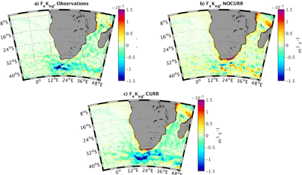
The Gulf Stream is assessed over the region: [76.2W - 38W; 31.8N 41.7N] and the Agulhas Current over the region:[2.5W - 48E; 43.2S 37.6S].

1.7 Coupling Coefficients

(30)

1.7.1 Current Feedback Coupling Coefficients

As in Renault et al. (2016d, 2017b), sτis defined as the slope of the robust regression (Li,

1985) between surface stress curl and oceanic current vorticity. It is evaluated at each grid point for both the simulations and the observations. The fields are first temporally aver-aged using a 29−day running mean to suppress the weather-related variability (Chelton et al., 2007), and the large-scale signal is removed using a high-pass Gaussian spatial filter with a 250 km cutoff (roughly corresponding to the eddy scale, as in e.g., Seo (2017), see filter description bellow). Note a e.g., 15−day running mean does not efficiently suppress the the weather-related variability.

sw is defined as the slope of the robust regression between 10-m (or ENW) wind curl and oceanic current vorticity. It is evaluated at each grid point for both the simulations and the observations. As for sτ, the fields are first temporally averaged using a 29−day

running mean and spatially filtered.

Table 1.2: Coupling Coefficients. sτ Surface current vorticity and surface stress curl

sw Surface current vorticity and wind curl sCstr Cross-wind SST and surface stress curl sCu Cross-wind SST and 10-m wind curl

sDstr Down-wind SST and Surface stress divergence sDu Down-wind SST and 10-m wind divergence sstr SST and Surface stress magnitude

su SST and 10-m wind magnitude

1.7.2 Thermal Feedback Coupling Coefficients based on Derivatives

Consistent with Chelton et al. (2007) and Wang and Castelao (2016), the following cou-pling coefficients have been estimated for the summer period of each hemisphere 10-m (or ENW): wind curl and cross-wind SST gradient (sCu); 10-m (or ENW) wind divergence and down-wind SST gradient (sDu); wind stress curl and cross-stress SST gradient (sCstr); wind stress divergence and down-stress SST gradient (sDstr). The method used here is similar to the one applied by Chelton et al. (2007) and Wang and Castelao (2016). Daily SST is used (a 3-day average does not change the result). The cross-wind (cross-stress) and down-wind (down-stress) components of the SST gradient is computed within each daily QuikSCAT wind UENWr (surface stress) and the daily SST. To remove the

(31)

atmo-and down-wind (cross-stress atmo-and down-stress) SST gradients, wind atmo-and surface stress curl and divergence. Anomalies of each variable are finally computed using a the spatial Gaussian high-pass filter (250−km cutoff, see above). Following such a method allows to reproduce, e.g., the Figure 1 from Wang and Castelao (2016). The same method is applied on the model fields.

1.7.3 Thermal Feedback Coupling Coefficients based on Mesoscale Anomalies

The coupling coefficients defined by ONeill et al. (2012) have been computed. They are based on mesoscale SST and the magnitude of wind (su) or surface stress (sstr). As in O’Neill et al. (2017), the influence of the storm have been damped out by removing large wind speed or surface stress magnitude with values greater than two standard deviations

σfrom the time mean at each grid point. This procedure allows removing potential biases

in the TFB response estimate that can be induced by the storm (atmospheric forcing vs. SST feedback). It removes less than 10 % of the points. The mesoscale anomalies are then estimated using the spatial filter described below.

1.8 Miscellaneous

1.8.1 10-m wind and Equivalent Neutral Wind

As described in the main text, we define 3 different sorts of wind:

— The relative wind Ur = Ua−Uo, with Uo being the oceanic surface current. Be-cause the first vertical level is often not defined around 10m, the 10-m wind is often diagnosed from the friction velocity and some atmospheric parameters. However, such a definition does not allow to estimate the absolute 10-m wind but rather the relative Ur.

— the 10-m wind Ua is defined as the first vertical level of the atmospheric model, which has been defined at≈10m.

— Satellite scatterometers (such as QuikSCAT) provide a 10m-wind, however it does not correspond to Ua: it is estimated from the pseudo-stress and is reported as the so-called Equivalent Neutral stability Winds (ENW, Bentamy et al. (2013)), i.e., the wind that would exist if the conditions were neutrally stable (Ross et al. (1985)). As confirmed in the manuscript, it actually represents the relative ENW to the surface current rather than the absolute ENW (UENWr). As in, e.g., Perlin et al. (2014), the UENWr is computed as:

UENWr = u∗ k (ln

10 z0

(32)

where the friction velocity u∗and roughness length z0(in meters) are taken at each output interval, and k =0.4 is the von Karman constant.

1.8.2 Submesoscale characterization

As in Capet et al. (2008c), the submesoscale is isolated from the signal using a high-pass spatial filter that consists of a five-point operator with a 12-km smoothing length and 2-days smoothing. Note, the use or not of the 2-days smoothing does not change qualitatively the results.

1.8.3 Spectrum

To compute the spectrum the area mean is first removed and a symmetrization is per-formed using an Hanning window Jenkins and Watts (1968).

1.8.4 Available Potential Energy

The mesoscale APE is estimated as Fox-Kemper et al. (2008); Srinivasan et al. (2017): APE = 1

2H 2

b|∇hbME|z, (1.21)

where bMErepresents the mesoscale component estimated using a spatial low-pass filter of 250 km, and the depth average is computed over the mixed layer depth Hb. Hb is estimated using the classic approach of the depth at which the density is 0.03 ◦C below that at 10 m depth (de Boyer Montégut et al. (2004)).

1.8.5 Surface Stress Induced Ekman Pumping

The Ekman pumping induced by the surface stress is computed as: wτ =k· ∇ ×

τ

ρ0 f , (1.22)

where f is the Coriolis frequency.

1.8.6 Spatial Filter

As described in Renault et al. (2017b), the mesoscale anomalies are isolated from the large scale signal by using a spatial filter. A field φ is smoothed using a Gaussian spatial filter with a standard deviation of 4 grid points. Gaussian weight of points located at a distance larger than 3σ are considered zero. The Gaussian filter is thus applied on a

(6σ+1)x(6σ+1)window which makes 25x25 points (≈6◦x 6◦) in our case. The cutoff of this filter is about 250 km. Land points are treated as missing data and the weights of windows including land points are renormalized over the remaining oceanic points.

(33)

field. Note the use of a larger filter cut-off would lead to similar results as this filter is applied on both SMTH and to the coupling coefficients described hereafter. Note the choice of the filter characteristics can also affect the strength of the coupling coefficient (in particular the one based on the mesoscale wind speed anomalies), however, it would not change the conclusion of this study.

(34)

Chapter 2 A Direct Control of the Oceanic

Circulation, from the Large Scale to the

Submesoscale

2.1 A Large Scale Effect: A Slow Down of the Gyre . . . . 33 2.2 At the Mesoscale: An "Eddy Killer" . . . . 38 2.2.1 A Dampening of the Mesoscale Activity . . . 38 2.2.2 Energy Conversion and Large Scale Sink of Energy . . . 40 2.3 At the Submesoscale: A Catalizer but Still a Killer, the case of the

Cali-fornia Current System . . . . 48 2.3.1 Dampening of the Submesoscale Activity . . . 50 2.3.2 A Submesoscale Sink of Energy . . . 51 2.3.3 A Catalizer of Submesoscale Baroclinic Instability . . . 55 2.3.4 Discussion . . . 55 2.4 Conclusion of the Chapter . . . . 58

(35)

The objectives of this Chapter are to assess how the current feedback direct effects on the ocean dynamic. In my recent research, I focused on 3 main direct effects: on the large scale, on the mesoscale, and on the submesoscale. The chapter is organized as follows: In Sec. 2.1 the direct effect of the current feedback on the mean circulation is assessed. I will use two examples: the North Atlantic Basin and the Greater Agulhas System. In Sec. 2.2, I will show how the current feedback plays a crucial role in determining the mesoscale activity. Finally, the submesoscale response will be addressed by focusing on the California Upwelling System in Sec. 2.3. The results are discussed and summarized in Sec. 2.4.

2.1 A Large Scale Effect: A Slow Down of the Gyre

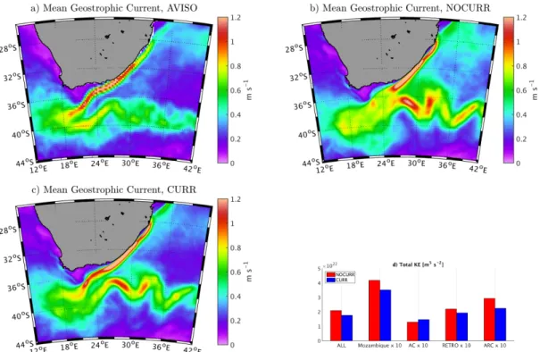
To illustrate the influence of the current feedback on the large scale circulation, I will consider in this section two different regions: the North Atlantic Basin, and the Greater Agulhas region (it encompasses the Mozambique channel, The Agulhas Current, and the Benguela Upwelling System). Both regions are characterized by an intense mean dynamic and by the presence of a Western Boundary Current: the Gulf Stream and the Agulhas Current, respectively. The results presented in this section have been published in the Journal of Physical Oceanography (JPO) (Renault et al. 2016c and Renault et al. 2017b).

The observed mean surface stress from the SCOW product (Scatterometer Climatol-ogy of Ocean Wind, Risien and Chelton 2008), is illustrated in Fig. 2.1a for the North Atlantic Basin. The surface stress is driven by the mean atmospheric circulation that is characterized by the presence of westerly and easterly winds in the north and south of the North Atlantic Basin, respectively. GS_CRT and GS_NOCRT have a good general representation of the mean surface stress, however, they both have a bias in the surface stress direction in the northwestern part of the domain, with a northward component overestimated with respect to the SCOW product (Fig. 2.1b). Because the mean cur-rents are moving in the same direction as the wind, from GS_CRT to GS_NOCRT, the current feedback reduces the mean surface stress up to 0.3 N m−2, where the currents are the strongest (τ = Cdρa(Ua−Uo)2 < Cdρa(Ua)2, where Cd is the drag coefficient). The weakening of the surface stress is realistic and reduces the biases with respect to the SCOW product (Fig. 2.1c).

The presence of the GS has a very clear effect on the surface stress curl. By weakening the surface stress, in GS_CRT, the current feedback reduces both the large scale negative and positive stress curl with respect to GS_NOCRT, improving the realism of the simula-tion (Fig. 2.2). In GS_NOCRT, consistent with the literature, the SST feedback produces a band of positive surface stress curl that is situated westward of the GS path (Fig. 2.2b).

(36)

There is an eastward positive SST gradient from the coast to the GS path (not shown). It induces a decrease of the surface stress (Chelton et al., 2004), and thus a positive stress curl, which is clearly overestimated with respect to SCOW (Fig. 2.2a). In GS_CRT, the SST feedback is still active, however, the current feedback produces an increase of the surface stress: the current vorticity is positive (Fig. 2.2a,b) and creates a negative surface stress curl (Renault et al., 2016d). It thus counteracts and dampens the SST feedback ef-fect, reducing the intensity of the positive band of surface stress curl along the U.S. East Coast. In the observations and in GS_CRT along the GS path, there is a band of positive stress curl that is not present in GS_NOCRT. Here, again, due to the current feedback, the surface stress is decreased along the GS path (Fig. 2.2ab), inducing a positive surface

Figure 2.1: Mean FmKmg(colors) and surface stress (arrows) estimated from the observations (a), GS_NOCRT (UNCOUPLED) (b), and GS_CRT (COUPLED) (c) for the period 2000-2004. In (c) the arrows represent the difference of mean surface stress between GS_NOCRT and GS_CRT (d) FmKmgaveraged over the whole domain (NATL), Gulf Stream (GS), and Center of the domain (CENTER), see black boxes on (a). The current feedback to the atmosphere decreases the surface stress and reduces FmKmg over the whole North Atlantic by 30%. Figure from Renault et al. (2016c).

(37)

stress curl.

Figure 2.2: The colors represent the mean surface stress curl from SCOW and from GS_NOCRT (UNCOUPLED) and GS_CRT (COUPLED) (for the period 2000-2004). The black contour shows the negative vorticity of the surface currents from AVISO and the simulations (contour of−3.10−7m s−1). The current feedback weakens the large scale surface stress curl and improves its realism. Due to the current feedback, the surface stress is decreased along the GS, inducing a positive surface stress curl collocated over the GS. Figure from Renault et al. (2016c).

Figure 2.1 depicts the FmKmg as estimated from the observations (using AVISO and SCOW) and the GS and AC simulations. The larger FmKmgvalues are situated along the westerlies and easterlies winds, where the current is also the strongest. Both GS_CRT and GS_NOCRT reproduce the main spatial pattern of FmKmg. By weakening the large scale surface stress, the current feedback induces a reduction of FmKmg (Fig. 2.1), in average by 30%. The main reduction occurs where the current is largest, i.e., the southwestern part of the gyre (including the Gulf of Mexico Loop Current), and the GS. GS_CRT still overestimates FmKmgwith respect to the observation estimates; this could be due partly to models biases but also to the spatial resolution and smoothing used in AVISO. The FmKmg reduction in GS_CRT is consistent with the Scott and Xu (2009) findings. Using the obser-vations, they suggest that ignoring the current feedback in the estimation of the surface stress leads to a systematic overestimation of FmKmg of 10% to 30%. The overestimation of FmKmg in GS_NOCRT compared to GS_CRT is about 50%, which is larger than the estimate by Scott and Xu (2009). However, although Scott and Xu (2009) uses the obser-vations that by definition include all the feedback Scott and Xu (2009) could not estimate the FmKmg for a non-active atmosphere that results in stronger oceanic currents. Figure 2.3 shows the depth integrated Kinetic Energy (KE) for GS_CRT and GS_NOCRT. The