Updating Failure Probability Of A Welded Joint In Offshore Wind Turbine Substructures

UPDATING FAILURE PROBABILITY OF A WELDED JOINT IN OFFSHORE WIND

TURBINE SUBSTRUCTURES

Aalborg University 9000 Aalborg Denmark Email: [email protected] Philippe Rigo Department of ArGEnCo/ANAST University of Liege 4000 Liege Belgium Email: [email protected] ABSTRACT

The operation and maintenance cost of offshore wind tur-bine substructures contributes significantly in the cost of a kWh. That cost may be lowered by application of reliability- and risk-based maintenance strategies and reliability updating risk-based on inspections performed during the design lifetime. Updating the reliability of a welded joint can theoretically be done using Bayesian updating. However, for tubular joints in offshore wind turbine substructures when considering a two dimensional crack growth and a failure criterion combining brittle fracture and ma-terial strength, the updating is quite complex due to the wind turbine loading obtained during operation. This paper solves that updating problem by using the Failure Assessment Diagram as a limit state function. It is discussed how application of the updating procedure can be used for inspection planning for off-shore wind turbine substructures, and thus also for reducing the required safety factors at the design stage.

NOMENCLATURE

FAD Fatigue Assessment Diagram

DFF Design Fatigue Factor

LEFM Linear Elastic Fracture Mechanics SIF Stress Intensity Factor

SCF Stress Concentration Factor

LSF Limit State Function

POD Probability Of Detection

⇤_{F.R.I.A. Ph.D. Student}

a Crack depth

c Semi crack length

t Plate thickness

KI Stress Intensity Factor in mode I

DK Stress Intensity Factor Range

Kmat Fracture Toughness

DKth Threshold value forDK

S Stress Range

C, m Parameters in Paris’ law CSN_,mSN _{Parameters in SN curves}

cd Detectable Crack Length

sY Yield Strength

su Ultimate Tensile Strength

sre f Reference Stress

Pb Primary Bending Stress

Pm Primary Membrane Stress

µ Mean

CoV Coefficient of Variation INTRODUCTION

For offshore wind turbines, the support structure contributes to a significant part of the Levelized Cost Of Energy (LCOE). LCOE is the total cost to build and operate a whole offshore wind turbine structure over its lifetime divided by the total energy out-put of the wind turbine over that lifetime. That total expected cost of operation & maintenance may be lowered by application Proceedings of the ASME 2016 35th International Conference on Ocean, Offshore and Arctic Engineering

OMAE2016 June 19-24, 2016, Busan, South Korea

of reliability- and risk-based maintenance strategies and updat-ing of the reliability based on e.g. inspections performed durupdat-ing the design lifetime. This maintenance strategy is also known as the conditioned maintenance that is optimized based on risk and pre-posterior Bayesian decision theory. Details about applying this cost optimal inspection and maintenance strategy to offshore wind turbines can be found in [1]. Basically it maximizes the final benefit of a wind turbine structure after considering all the costs (i.e. fabrication, inspection, repair, maintenance, strength-ening, and failure costs) and it is subjected to the condition that the failure probability at a certain year is not larger than a maxi-mum annual failure probability. In order to do that, the updated failure probability of the structure or component must be calcu-lated considering various decisions taken modelled by decision rules — possible repair/maintenance actions.

Updating the reliability (or alternatively the failure probability) of a welded joint in the wind turbine support structure can theo-retically be done using Bayesian updating. However, for tubular joints of offshore wind turbine substructure, when considering a two dimensional crack growth and a failure criterion combining brittle fracture and material strength, the updating is quite com-plex due to the wind turbine loading obtained during operation. In [2], the authors used the Failure Assessment Diagram (FAD) as a limit state function and successfully performed the relia-bility updating based on inspections and repairs. However, the geometry function was assumed constant for crack propagation and an assumption of lognormal distribution for crack size was made in calculating reliability index using First Order Reliability Method.

This paper considers how the reliability (or the probability of failure) of welded steel details can be updated in the case where the fatigue failure is modelled by a fracture mechanics approach and a FAD is used to define the limit state equation. A two di-mensional bi-linear model is considered for the crack growth. Calculation of the crack depth and the crack length are cou-pled. The stress intensity factor is calculated following the BS 7910:2005 [3] sophisticated procedure. The initial crack size, the yield and ultimate strengths of steel, the fracture toughness, the stress intensity factor, and the stress-ranges are considered as uncertain and modelled by random variables. The probability of detection is used to represent the uncertainty in crack inspec-tions. By using Monte Carlo simulations, stress-range histories are generated randomly and together with the calculated stress intensity factors to check the limit state condition using the FAD approach. The result of failure probability from FAD approach is compared with the one from the conventional limit state function. The updating of the failure probability is done for three inspec-tion scenarios: No crack detected; Crack detected and repaired; Crack detected and not repaired.

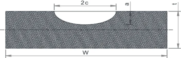
a

2 c t

W

FIGURE 1: ILLUSTRATION OF CRACK DIMENSIONS

CRACK GROWTH MODELLING

In damage tolerant design, welded joints are considered as imperfect even before they are put in service. This is because of the uncertainty/imperfections in material properties and man-ufacturing. Those imperfections work as initial cracks that may grow under the hash environmental loading and become critical for the failure of the joints as well as the whole structure.

To model the crack growth over time, this paper will use the Paris-Erdogan law [4]. Although Paris-Erdogan law is only valid for long cracks in LEFM and uniaxial loading conditions, it is widely used in offshore practice (e.g. as in DVN-GL, BS 7910, IIW, HSE [3, 5–7] ) thanks to its simplicity in input parameters and sufficient accuracy.

The crack growth of an initiated crack due to an imperfection is assumed to be a ‘long crack’, corresponding to the stable crack region in the Paris-Erdogan law as in Eqn. (1), where C and m are treated as material parameters for a given mean stress and environmental condition. DK is the stress intensity factor range at the crack tip, corresponding to the applied nominal stress range S, see next section.

da dN =Ca(DKa)m forDKa>DKth (1) dc dN =Cc(DKc) m _forDK c>DKth (2)

Equation (1), which is used for a surface crack to find the crack depth a, will be coupled to equation Eqn. (2), which is another crack front direction to find the crack length 2c — the end points of the crack at the surface. It is important to have accurate values for two random variables a and c since the crack length is what can be measured during inspections while the crack depth a is what is usually considered in the failure criteria. Figure 1 illus-trates crack depth and crack length for a surface crack, where t and W are thickness and width of the steel plate. DKth in

Eqns. (1) and (2) is the threshold value below which the crack is assumed to be non-propagating.

Stress Intensity Factor (SIF) Range

Although many problems for welded joints are of the mixed mode type, mode 1 is considered as the dominant mode for fa-tigue propagation and fracture. The SIF range is calculated from Eqn. (3) for crack depth and from Eqn. (4) for crack length, where Yaand Ycare stress intensity correction factors calculated

following BS 7910 [3].

DKa=SYappa (3)

DKc=SYcppa (4)

Stress Ranges

Normally, stress-range is considered as a constant value named “Weighted Average Stress Range” as calculated in Eqn. (5) from its distribution. This is based on linear damage accumulation principle and can be used for fatigue life calcula-tion in both SN approach and FM approach [8].

SemSN=SmSN= • Z 0 SmSN f (s)ds (5)

In this paper, we consider the crack propagation in a “realistic” loading condition, i.e. the stress ranges are generated randomly based on the operating characteristics of wind turbines to be used as representative constant values for short periods of time.

For offshore structures, the long term stress ranges are of-ten represented by a two-parameter Weibull distribution. As the joint considered in this paper is in a jacket support structure of an offshore wind turbine, it is reasonable to assumed the Weibull shape parameter to be 0.8 as suggested in [5]. The scale parame-ter is assumed normally distributed with CoV=15% and the mean value is calibrated based on the design fatigue factor (DFF) of the joint.

PROBABILITY OF DETECTION

The probability of detection, POD, expresses the probability of detecting a crack of a given length (2c). It is a parameter to evaluate the accuracy of an inspection technique. Three different POD curves [9] are illustrated in Fig. 2. Curve 1 incorporates the possibility of non-detection of large cracks. Curve 2 incor-porate false call probability — it is the fraction of time that an un-cracked joint will be incorrectly classified as being cracked. Curve 3 ignores the possibility of false calls and non-detection of large cracks and normally used as a cumulative distribution function in Bayesian updating for failure probability of a joint.

Curve 1: Incorporate the possibility of non-detection of large cracks Curve 2: Incorporates false call probability Curve 3: Ignores the possibility of false calls

and non-detection of large cracks 1 POD( a) 0 Crack size a 3 2 1

FIGURE 2: TYPES OF POD CURVE

Although Curve 1 and Curve 2 are not in the form of a cumu-lative distribution function, they can easily be incorporated in updating the failure probability.

POD(cd) =1 exph c_ld

i

(6) For illustration purpose, this paper uses the POD — a function of the smallest detectable crack length in [mm] — as in Eqn. (6), with the parameter l = 1.95 corresponding to a quite good in-spection technique for tubular joints in sea water [10].

LIMIT STATE EQUATION

Limit state equations for fatigue assessment of a surface crack can be defined in both serviceability and ultimate limit sates. Two examples of failure criteria can be considered [11] as shown in Eqn. (7) and Eqn. (8) .

ac a  0 (7)

Kmat KI 0 (8)

A critical crack size acis selected in the first case, Eqn. (7),

e.g. based on serviceability considerations. In the second case, Eqn. (8), the fracture toughness Kmat of material is used as a

critical value for the stress intensity factor KI. When Eqn. (8)

happens, the crack growth becomes unstable and rapid failure oc-curs. It is worth mentioning that the stress intensity factor is used for fracture assessment while the stress intensity factor range is used for crack propagation. The stress intensity factor is calcu-lated similar toDKaas in Eqn. (3) but the stress range is replaced

by the maximum applied stress.

For redundant structural systems like jacket platforms, finding ac

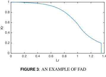
based on serviceability is time consuming but assuming failure in the full plate thickness may be too conservative. Another ap-proach would be using the interactive diagram combining two failure criteria: linear elastic fracture mechanics (LEFM) and plastic collapse — the Fatigue Assessment Diagram of BS 7910 [3]. According to this standard, there are three assessment levels in terms of available information. While Level 1 is a conservative assessment with limited information about material and applied stresses, Level 3 is a complex assessment for ductile materials. The normal assessment route for general application is Level 2. Depends on the availability of the stress/strain data, this level is subdivided into Level 2A and Level 2B. The assessment in this paper follows the procedure for Level 2A — assuming that the stress-strain curve is not available. Following this procedure, the assessment line is given by the equation of a curve and a cutoff as illustrated in Fig. 3. If the assessment point lies within the area bounded by the axes and the assessment line, the crack is acceptable, otherwise it is unacceptable. The cutoff is to prevent localized plastic collapse and it is set at Lr=Lmaxwhere Lmaxis

defined as in Eqn. (9).

Lmax=sY_2s+su

Y (9)

The equations describing the assessment line (Fig. 3) are the fol-lowing: For Lr<1 : Kr= 1 0.14L2r h 0.3 + 0.7exp⇣ 0.65L6r ⌘i (10) For 1 < Lr Lrmax: Kr=Kr(Lr=1)L(N 1)/(2N)r (11) where N = 0.3⇣1 sY su ⌘

is the strain hardening exponent estimated from the yield to tensile strength ratio,sY/su.

For Lr>Lrmax:

Kr=0 (12)

The assessment point is positioned by the two coordinates Krand

Lras in Eqns. (13 ) and (14). Kr= KI Kmat (13) Lr 0 0.2 0.4 0.6 0.8 1 1.2 1.4 Kr 0 0.2 0.4 0.6 0.8 1

FIGURE 3: AN EXAMPLE OF FAD

Lr=s_sre f

Y (14)

wheresre f is obtained from Eqn. (15) for a weld toe crack

sre f= Pb+ n P2 b+9Pm2(1 a00)2 o0.5 3(1 a00₎2 (15)

with Pm, Pbare primary membrane stress and primary bending

stress, respectively; and: ( a00_{= (a/t)/{1 + (t/c)} for W 2(c +t)} a00_{= (2a/t)(c/W ) for W < 2(c +t)} (16) UNCERTAINTIES

Beside the uncertainties associated to the detectable crack length and stress ranges, other variables need to be considered as uncertain. These are initial crack sizes, yield and ultimate strengths, fracture toughness, SIF, and threshold value of SIF. Initial Crack Size

The initial defects in modern fabricated welds are assumed to be extremely small, typically less than 10 µm (0.01 mm). These cracks are too small that LEFM is not applicable. Before reaching a depth of 100 µm, they grow faster than LEFM pre-dicts. Normally the time for a crack depth reaches 100 µm is con-sumed in short crack propagation, and it is about 20 % to 30 % of the fatigue life [8]. For welded joints in substructures of offshore wind turbines, it is sufficient to consider only crack depths above 100 µm — long crack propagation — where LEFM is applicable to model the propagation phase until failure is reached.

However, it is mentioned in [12,13] that the mean value and stan-dard deviation of initial crack depth a0 can be estimated to be

0.15 mm and 0.10 mm, respectively, for ”sound” quality welds. It has been fitted to weld defect data using Lognormal, exponen-tial and Weibull distributions. For the iniexponen-tial crack length, it is suggested to use initial defect aspect ratio, which is defined as the ratio of initial crack depth to semi crack length (a/c). This quantity may also be modelled as a lognormal random variable with a mean of 0.62 and CoV of 0.4 as suggested in [12]. For cracks that need to be repaired after inspection, this paper considers two cases for the new initial crack depth — either crack is repaired perfectly or as after-fabricated state.

Yield and Ultimate Strengths

Uncertainties of Yield and Ultimate Strengths are often as-sumed to follow a normal, lognormal, or a Weibull distribution [14–16]. By fitting an extensive data set of the yield strength from the English Health and Safety Executive materials database to normal, lognormal, and Weibull distributions, it was found that the lognormal distribution was the most appropriate one [16]. According to [15, 17], the parameters of the lognormal distribu-tion for yield and ultimate tensile strengths can be calculated in two cases:

If only measured mean values for yield strength (µsY)and

ultimate tensile strength (µsu)are available, the standard

de-viation values are determined as: - yield strength:

ssY =0.03µsY (17)

- ultimate tensile strength:

ssu =0.05µsu (18)

If only standardized values for yield strength (Re)and

ulti-mate tensile strength (Rm)are available, the mean and

stan-dard deviation values are determined as: - yield strength:

µsY =Re+70MPa and ssY =30MPa (19)

- ultimate tensile strength:

µsu =Rm+70MPa and ssu=30MPa (20)

In JCSS [12], the mean and coefficient of variation values of yield and ultimate tensile strengths are calculated as:

- yield strength:

µsY =fysp· a · exp( u ·CV) C (21)

CoVsY=0.07 (22)

- ultimate tensile strength:

µsu=Bt· E[ fu] (23)

CoVsu=0.04 (24)

where

fysp the code specified or nominal value for the yield

a spatial position factor (a = 1.05 for webs of hot rolled sec-tions anda = 1 otherwise)

u is a factor related to the fractile of the distribution used in describing the distance between the code specified or nom-inal value and the mean value; u is found to be in the range of 1.5 to 2.0 for steel produced in accordance with the relevant EN standards; if nominal values are used for fysp,

the value of u needs to be appropriately selected.

C is a constant reducing the yield strength as obtained from usual mill tests to the static yield strength; a value of 20MPa is recommended.

Bt is a factor, Bt=1.5 for structural carbon steel; Bt=1.4 for

low alloy steel; Bt=1.1 for quenched and tempered steel.

This paper considers the method suggested by JCSS [12] to cal-culate parameters of the lognormal distributions of yield and ul-timate tensile strengths. fysp=350MPa is chosen as the nominal

value of the yield strength, E[ fu] =500MPa,a = 1, u = 1.5,

and B = 1.5 implies that:µsY =368.75MPa andµu=750MPa.

Fracture Toughness

Fracture toughness is a property describing the ability of a material containing a crack to resist fracture. The fracture tough-ness can be represented either by KIc- the critical stress intensity

factor for a brittle failure or by JIc- the critical energy for a

duc-tile failure. For weld-toe cracks of offshore structures, the KIcis

of interest. When the stress intensity factor K exceeds fracture toughness, the crack growth becomes unstable and rapid failure occurs. Fracture toughness is found by doing laboratory tests at various temperatures. At each temperature, there are a lot of samples tested to find the fracture toughness. In the lower shelf and transition region, Wallin [18] and others have argued for the

use of Weibull distribution for the tested results.

A three-parameter Weibull distribution is proposed to describe fracture toughness related to cleavage fracture [12, 17, 19]

FKmat(k) = 1 exp " ✓ k K0 Ak ◆Bk# (25) where:

Bk is the shape parameter, taken as 4 on the basis of experiments

[17];

K0 is the threshold parameter, a recommended value is

20 MPa m1/2_[19];

Ak is the scale parameter and can be calculated from Eqn. (26)

[12]. Ak= ⇢ 11 + 77  exp✓ T T27J+T0 52 ◆ _{✓ 25} t ◆1/4 (26) T is operating temperature ( C), chosen to be e.g. 5 C. T27J is temperature ( C) corresponding to a Charpy V-Notch of

27 J, chosen to e.g. 50 C

T0 is modelling variability of T27J: e.g. Normal distributed with

mean of 18 C and standard deviation of 15 C; t is plate thickness in mm.

SIF, SCF and SIF Threshold

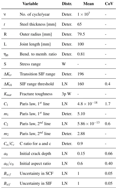
Since these parameters are established from finite element analyses and experiments, SIF, SCF and SIF threshold should be considered as uncertainties in calculating the failure probability of the joint. Using the suggestion of JCSS [12], the stochastic models in Tab. 1 are used.

APPLICATION

To demonstrate the failure probability updating procedure using the FAD as a limit state function, a tubular joint with all the input data as shown in Tab. 1 is chosen. The joint is assumed to be placed in air conditions, and is designed using the SN ap-proach with DFF = 3 for a service life of 20 years. The bi-linear SN curve is used for fatigue design of the joint, taken from [20] and shown in Tab. 2.

The uncertainty in assessment of the stress ranges is represented by the scale parameter (k) of the Weibull distribution for the long term stress range distribution. It is normally distributed with CoV = 15% and the mean value is calibrated from the DFF value in SN approach (µk= 6.5766 MPa). Randomly generated values of

the stress ranges will be considered as a constant value during a short period of time for crack propagation. This generated stress

TABLE 1: INPUT VARIABLES FOR CRACK PROPAGATION

Variable Distr. Mean CoV

n No. of cycle/year Deter. 1 ⇥ 107

-t Steel thickness [mm] Deter. 65

-R Outer radius [mm] Deter. 79.5

-L Joint length [mm] Deter. 100

-hs Bend. to memb. ratio Deter. 0.81

-S Stress range W -

-DKtr Transition SIF range Deter. 196

-DKth SIF range threshold LN 160 0.4

Kmat Fracture toughness 3p W -

-C1 Paris law, 1stline LN 4.8 ⇥ 10 18 1.7

m1 Paris law, 1stline Deter. 5.10

-C2 Paris law, 2ndline LN 5.86 ⇥ 10 13 0.6

m2 Paris law, 2ndline Deter. 2.88

-Ca/Cc C ratio for a and c Deter. 0.9

-a0 Initial crack depth LN 0.15 0.66

a0/c0 Initial aspect ratio LN 0.6 0.40

Bsc f Uncertainty in SCF LN 1 0.05

Bsi f Uncertainty in SIF LN 1 0.05

Note: Deter. = Deterministic; W = Weibull distribution; 3p W = Three parameter Weibull distribution; LN = Lognormal distribution;

range history will be used together with other results of simula-tion i.e. a, c,DKa,DKc, Kmat to assess failure of the joint using

the FAD.

For illustration, inspections will be performed at years 5, 10, and 15. Three scenarios will be considered: no crack detected; crack detected and repaired; crack detected and not repaired.

TABLE 2: THE DESIGN SN CURVE SN Curve N 1 ⇥ 10 7_{cycles N >1 ⇥ 10}7_cycles mSN 1 logC1SN mSN2 logC2SN T 3.0 12.164 5.0 15.606

RESULTS AND DISCUSSION

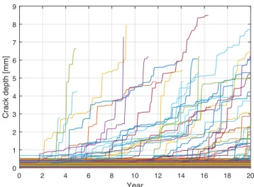
1 ⇥ 106_{samples of crack propagations are simulated for the}

chosen joint (see Fig. 4) for assessment of the failure probability. Figures 5 and 6 show that the solution converges for the chosen number of samples. In this section, results are shown to compare the FAD limit state function and the conventional one; to indi-cate the importance of doing inspections during the service life; to show the effects of repair quality; and to predict conditional failure probability if crack detected and not repaired.

Realizations of the crack propagation are ‘filtered’ during the simulations using three conditions:

- Crack depth is not larger than the steel thickness. Due to the way stress range is generated, it may happen that the crack depth in the next month will be larger than the thickness. Since we consider only surface cracks, the result of crack propagation will be reported up to the current month, even if the crack depth is still smaller than the critical value. - The second condition is a restraint on the crack length. It is

required that the crack length be not larger than 80% of the tubular perimeter so that the formulation of bulging effects is applicable [3].

- The third condition is about fracture toughness. It can be seen that when K Kmathappens, the assessment point will

be in the failure region of the FAD. From that point on, the results of crack propagations will be classified in the failure region. This condition helps to save the simulation time.

Advantages of FAD Limit State Function

The failure probability is calculated using two approaches on the ‘filtered’ set of samples:

- The conventional approach — using the critical crack depth and fracture toughness as criteria as shown in Eqns. (7) and (8).

- The FAD approach — using the assessment line as shown in Fig. 3 to check whether the sample point stays in the safety region. Year 0 2 4 6 8 10 12 14 16 18 20 Crack depth [mm] 0 1 2 3 4 5 6 7 8 9

FIGURE 4: ILLUSTRATION OF CRACK PROPAGATION

Number of sample 100 101 102 103 104 105 106 Probability of failure #10-3 0 0.2 0.4 0.6 0.8

1 Convergence of the MCS solution

FIGURE 5: CUMULATIVE PFAFTER THE FIRST YEAR

Using FAD on the safety region of the conventional limit sate function gives additional failures as shown in Tab. 3. This table indicates number of samples failed in additional to those found by the conventional LSF. Two failure criteria are differen-tiated (i.e. Kr Krcrit and Lr Lmaxr ) in order to find the cause

of failure. Table 3 shows that Lris always smaller than the Lmaxr

for the whole life, but the fracture ratio (i.e. Kr=KI/Kmat) is

not always smaller than the critical value in FAD. All the assess-ment points are in the safety region of the conventional LSF (i.e. KI<Kmat and a < ac) but some of them are classified as failure

in the FAD approach since they lie above the assessment curve. It means that FAD is stricter than the conventional limit state

func-TABLE 3: ADDITIONAL FAILURE FOUND BY USING FATIGUE ASSESSMENT DIAGRAM Criteria Year 1 2 3 4 5 6 7 8 9 10 11 12 13 14 15 16 17 18 19 20 Kr Krcrit 0 0 0 0 0 0 0 0 0 0 0 2 1 3 1 0 0 1 0 0 Lr Lmaxr 0 0 0 0 0 0 0 0 0 0 0 0 0 0 0 0 0 0 0 0 Number of sample 103 104 105 106 Probability of failure 0.05 0.055 0.06 0.065

0.07 Convergence of the MCS solution

FIGURE 6: CUMULATIVE PF AFTER THE YEAR 20th

tion in defining a safety region.

In addition, a crack depth that is larger than the plate thickness does not necessarily indicate that a failure happens since the re-maining cross-section may still be able to carry the load. How-ever, in assessing failure of joints with those cracks, the conven-tional LSF would not be applicable. On the other hand, FADs are available for assessing various crack types [3], so using FAD as a limit state function would help to assess the failure probability of larger crack sizes.

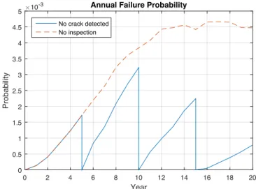
No Crack Detected

Figure 7 shows the annual failure probability of two cases: when ‘no inspection is performed’ and ‘with inspection but with-out any crack detected’. If the maximum allowable annual failure probability of the joint is 5 ⇥ 10 3_{then the chosen joint may be}

in the risk of violating this Pf value. In order to prevent that, we

perform inspections at years 5, 10, and 15. The result shows that

Year 0 2 4 6 8 10 12 14 16 18 20 Probability #10-3 0 0.5 1 1.5 2 2.5 3 3.5 4 4.5

5 Annual Failure Probability

No crack detected No inspection

FIGURE 7: ANNUAL PF— NO CRACK DETECTED

the maximum annual failure probability is reduced from near-critical value to about 3.2 ⇥ 10 3_{. The accumulated failure}

prob-ability is reduced a lot thanks to the inspections as shown in Fig. 8.

Crack Detected & Repaired

If during an inspection, a crack length is larger than or equal to the detectable size then that crack is detected. Depending on the decision rule, that crack may be let to grow or it is repaired by grinding or welding. To see the importance of welding quality, we compare the updated failure probability for ‘normal’ repair and ‘perfect’ repair. ‘Normal’ repair makes the weld back to the state as after manufacturing, i.e. there is a possibility of having other initial cracks, while ‘perfect’ repair makes the weld be as good as crack-free. In incorporating the effects of repair to the simulations, the remaining part of a sample from where a crack is detected will be replaced by a new one for ‘normal’ repair or

Year 0 2 4 6 8 10 12 14 16 18 20 Probability 0 0.01 0.02 0.03 0.04 0.05 0.06

0.07 Cumulative Failure Probability

No crack detected No inspection

FIGURE 8: CUMULATIVE PF— NO CRACK DETECTED

Year 0 2 4 6 8 10 12 14 16 18 20 Probability #10-3 0 0.5 1 1.5 2 2.5 3

3.5 Annual Failure Probability

Normal Repair Perfect Repair

FIGURE 9: ANNUAL PF— DETECTED & REPAIRED

will not be counted in calculating failure probability for ‘perfect’ repair. Figures 9 and 10 show that ‘perfect’ repair helps to a larger reduction of the failure probability after each inspection than ‘normal’ repair. This effect can be seen more clear at the end of the service life.

Crack Detected & Not Repaired

Updating the failure probability of the joint when a crack is detected but not repaired is performed on the realizations of crack propagation. In this event, the updated failure probability is conditioned on a certain detected and measured crack size (e.g. a=2 cm in the first inspection). The magnitude of the result is

Year 0 2 4 6 8 10 12 14 16 18 20 Probability 0 0.005 0.01 0.015 0.02

0.025 Cumulative Failure Probability

Normal Repair Perfect Repair

FIGURE 10: CUMULATIVE PF— DETECTED & REPAIRED

about 10 6_{for the conditionally updated failure probability after}

5 years, so it requires much more samples to converge. Another approach to update failure probability when crack detected and not repaired can be FORM as in e.g. [2]. However, in order to use FORM with the FAD limit state function, one will need to know in advance the distribution of crack size because it is an important variable to calculate fracture factor (Kr) and the reference stress

in FAD. It should be mentioned that even if the updated failure probability conditioned on this observation (i.e. crack detected and not repaired) can be found, it is difficult to use that result to plan future inspections because of very large computational times.

CONCLUSION

In this paper, fatigue failure probabilities of tubular joints in substructures of offshore wind turbine are updated after in-spections. Failure probabilities are calculated using the Fatigue Assessment Diagram and compared with the conventional limit state function. The crack propagations are calculated using a bi-linear Paris’ law with stress range values vary with time. Calcu-lations of crack length and crack depth are coupled. The FAD limit state function is used successfully with the simulation ap-proach to update the failure probability of the joint in two in-spection scenarios: ‘no crack detected’, ‘crack detected and re-paired’. For the ‘case crack detected but not repaired’, updating failure probability looks to be too much time consuming with simulation approach.

Results of calculations show that for surface cracks, FAD and the conventional LSFs give similar failure probabilities. However, FAD is stricter than the conventional one in defining a safety re-gion and can be used to assess failure for crack depths larger than

plate thickness. The FAD approach showed to work well in up-dating failure probability of a joint.

This FAD approach can be used further in inspection planning for offshore wind turbine support structures, to include systems effects and thus also for reducing the required safety factors at the design stage.

ACKNOWLEDGMENT

This research is funded by the National Fund for Scientific Research in Belgium — F.R.I.A - F.N.R.S.

REFERENCES

[1] Sørensen, J., 2009. “Framework for Riskbased Planning of Operation and Maintenance for Offshore Wind Turbines”. Wind energy, 12(5), pp. 493–506.

[2] Yeter, B., Garbatov, Y., and Soares, C. G., 2015. “Fatigue Reliability of an Offshore Wind Turbine Supporting Struc-ture Accounting for Inspection and Repair”. In Analysis and Design of Marine Structures, G. Soares and Shenoi”, eds., Taylor & Francis Group, London, pp. 737–747. [3] BS-7910, 2005. Guide to Methods for Assessing the

Ac-ceptability of Flaws in Metallic Structures. British Standard Institution (BSi).

[4] Paris, P., and Erdogan, F., 1963. “A critical analysis of crack propagation laws”. Journal of Basic Engineering,85, pp. 528–534.

[5] DNVGL-RP-0001, 2015. Probabilistic Methods for Plan-ning of Inspection for Fatigue Cracks in Offshore Struc-tures. Det Norske Veritas & Germanischer Lloyd Group (DNV GL), May.

[6] Hobbacher, A., 2008. Recomendations for Fatigue Design of Welded Joints and Components. Tech. Rep. IIW doc-ument IIW-1823-07 ex XIII-2151r4-07/XV-1254r4-07, In-ternational Institute of Welding (IIW).

[7] Aker Offshore Partner A.S, 1999. Target Levels for Reliability-based Assessment of Offshore Structures Dur-ing Design and Operation. Tech. Rep. 1999/060, Health & Safety Executive (HSE).

[8] Lassen, T., 1997. “Experimental Investigation and Stochas-tic Modelling of the Fatigue Behaviour of Welded Steel Joints”. Ph.d. thesis, Aalborg University, Aalborg.

[9] Simonen, F. A., 1995. “Nondestructive Examination Reli-ability”. In Probabilistic Structural Mechanics Handbook, C. R. Sundarajan, ed., Springer, pp. 238–260.

[10] Moan, T., and V˚ardal, O., 1997. “In-service Observations of Cracks in North Sea Jackets. A Study on Initial Crack Depth and POD Values”. In Proceeding on 16th OMAE conference, Yokohama, Japan., American Society of Me-chanical Engineers (ASME), pp. 189–198.

[11] Madsen, H. O., Krenk, S., and Lind, N. C., 2006. Methods of Structural Safety. Courier Dover Publications.

[12] JCSS, 2001. Probabilistic Model Code: Part 3 Resistance Models. Joint Committee on Structural Safety (JCSS). [13] Kountouris, I., and Baker, M., 1989. Reliability of

Non-destructive Examination of Welded Joints. Imperial College of Science and Technology Engineering Structures Labora-tories.

[14] British Energy, 2001. R6: Assessment of the Integrity of Structures Containing Defects, revision 4 ed. British En-ergy Generation Ltd., Gloucester.

[15] Dillstrom, P., 2000. Probabilistic Safety Evaluation-Development of Procedures with Applications on Compo-nents Used in Nuclear Power Plants. Tech. Rep. 00:58, Swedish Nuclear Power Inspectorate (SKI).

[16] Burdekin, F., and Hamour, W., 1998. “SINTAP, Contribu-tion to Task 3.5, Safety Factors and Risk”. UMIST, 25p. [17] Wallin, K., 1998. “Probabilistisk sakerhetsvardering

propse-materialparametrar”. Rapport VALC444, VTT Tillverkningsteknik, p. 22.

[18] Wallin, K., 1999. “The Master Curve Method: a New Con-cept for Brittle Fracture”. International Journal of Materi-als and Product Technology, 14(2-4), pp. 342–354. [19] Burdekin, F., and Hamour, W., 2000. Partial Safety Factors

for the SINTAP Procedure. Health and Safety Executive (HSE).

[20] DNVGL-RP-0005, 2014. RP-C203: Fatigue Design of Off-shore Steel Structures. Det Norske Veritas & Germanischer Lloyd Group (DNV GL), June.