Inequality in Exposure to Air Pollution in France: Measurement and Impact of a City-Level Public Policy

(1)

HAL Id: dumas-03045169

https://dumas.ccsd.cnrs.fr/dumas-03045169

Submitted on 7 Dec 2020

HAL is a multi-disciplinary open access archive for the deposit and dissemination of sci-entific research documents, whether they are pub-lished or not. The documents may come from teaching and research institutions in France or abroad, or from public or private research centers.

L’archive ouverte pluridisciplinaire HAL, est destinée au dépôt et à la diffusion de documents scientifiques de niveau recherche, publiés ou non, émanant des établissements d’enseignement et de recherche français ou étrangers, des laboratoires publics ou privés.

Inequality in Exposure to Air Pollution in France:

Measurement and Impact of a City-Level Public Policy

Pascale Champalaune

To cite this version:

Pascale Champalaune. Inequality in Exposure to Air Pollution in France: Measurement and Impact of a City-Level Public Policy. Economics and Finance. 2020. �dumas-03045169�

(2)

MASTER THESIS N° 2020 – 01

Inequality in Exposure to Air Pollution in France:

Measurement and Impact of a City-Level Public Policy

Pascale Champalaune

JEL Codes: I14, Q53, Q56, R23

Keywords: Air pollution, Environmental Economics, Inequality, Spatial

autocorrelation

(3)

Inequality in Exposure to Air Pollution in France:

Measurement and Impact of a City-Level Public Policy

Master’s Thesis Pascale Champalaune

M2 APE, Paris School of Economics September 2020

Supervisors: Lucas Chancel & Thomas Piketty

Abstract

I combine measures of neighbourhood characteristics with high-resolution remote-sensing data

to provide the first national-scale study of cross-sectional and longitudinal inequality in ex-posure to fine particulate matter (PM_2.5) in France. Descriptive evidence indicates that,

at the national level, there is a U-shaped relationship between income and PM2.5 exposure,

which is not reflected within urban areas. Fixed-effect models confirm that on average, higher

neighbourhood income is associated with lower exposure. Longitudinal inequality measures suggest that recent air quality improvements accrued predominantly to areas that had a lower

initial exposure, and intermediate income. I then exploit a change in air quality schemes at the level of urban areas in an event-study framework, so as to shed light on potentially

un-equal benefits from the induced reduction in exposure. I find that initially lower-income areas received smaller benefits from the policy change, and quantile regression estimates suggest

that exposure decreased more in less polluted areas. As some results are sensitive to formally accounting for spatial autocorrelation, this study also underlines the need to pay specific

attention to this issue when measuring environmental inequality.

JEL Codes: I14, Q53, Q56, R23

Keywords: Air pollution, Environmental Economics, Inequality, Spatial autocorrelation

I thank François Fontaine, François Libois, and Louis Sirugue for their time and very helpful comments and suggestions. I am particularly grateful to Lucas Chancel and Thomas Piketty, who supervised this Master’s Thesis, and to Camille Hémet, who accepted to act as referee, for their support.

(4)

1 _Introduction

As public goods, environmental amenities are an integral part of the real income of households. This makes their distribution part of the general panorama of inequality. More specifically, unequal

access to clean air may reinforce preexisting health inequalities, both across space and across income groups. Despite both policy-makers and the general public showing growing concern about it, the

French economic literature on the issue is still in its infancy. In addition, over the last two decades, the country recorded substantial air quality improvements, driven in part by long-term technological

development, and in part by dedicated policies. It is thus necessary to evaluate whether the latter benefitted all individuals to the same extent.

1.1 _{Main contributions}

The contribution of this study to the academic literature is threefold. First, I provide the first nationwide evidence of cross-sectional and longitudinal inequality in exposure to fine particulate matter (PM_2.5). In mainland France, the associated health burden was recently estimated to 48,000

early deaths a year, which is equivalent to 2-year reduction of life expectancy at 30 on average (Medina et al., 2016). Albeit these detrimental health impacts, this pollutant has been overlooked

by the French literature on environmental inequality, partly due to the fact that there were very few PM_2.5 monitors in France prior to the 2010s. I thus contribute in filling this gap by exploiting

high-resolution satellite data, coupled with census block-level INSEE data. This allows the study not only to cover the whole of metropolitan France, but to do so at a fine spatial granularity. This

is particularly crucial so as to limit the risk of ecological fallacy, i.e., to avoid making erroneous inference on individual correlations based on neighbourhood correlations (Banzhaf et al., 2019).

I show that, at the national level, there is a U-shaped relationship between PM2.5 exposure

and income, which is not reflected within urban areas, where only the lowest income deciles face

a disproportionate burden of exposure. I tackle the omitted variable bias related to unobserved neighbourhood heterogeneity using fixed-effect models, and confirm that there is indeed a negative

relationship between the two variables of interest in France. The results also suggest that the share of immigrants is positively associated with PM_2.5concentration, hinting at an ethnic gap in exposure

reminiscent of that observed in the United States. I also contribute to the literature by providing longitudinal measures of inequality, and present evidence that census blocks that benefitted from

(6)

located either at the lower or upper end of the distribution of income. This study thus uncovers

that despite the fact that PM2.5 exposure dropped throughout the country between 2006 and 2016,

there is growing inequality in its distribution.

My second contribution consists in taking advantage of a policy change that occurred at the level of urban areas, in order to investigate whether new PM_2.5 regulation played a role in this

evolution. In France, since the 1996 LAURE law, part of the regulation of air quality is effected by the local authorities of the largest cities, through Plans de Protection de l’Atmosphère. Following

the 2008 EU Directive on ambient air quality and cleaner air for Europe, urban areas had to revise their schemes so as to newly include measures aimed at reducing PM_2.5 concentration. Given that

the years of implementation vary from 2012 to 2016, I make use of an event-study design in order to analyse how inequality in exposure to air pollution evolved as a consequence of this change. In line

with the abovementioned findings, I demonstrate that these revised plans predominantly benefitted initially advantaged neighbourhoods, i.e., those whose income lay above the median. In addition, I

provide quantile regression estimates which suggest that lower quantiles of exposure received larger air quality improvements.

As a third contribution, throughout this study, I pay specific attention to the robustness of

the results to formally accounting for spatial autocorrelation, as opposed to most of the economic literature in the field of environmental inequality. Concomitantly, I provide a concise review of

the methods used in Public Health studies, and argue that the spatial lag model, which seems the most widespread, relies on arbitrary parametric assumptions that may threaten the validity of

the estimates. I thus rely on a non-parametric approach to model spatial autocorrelation, using a smoothing spline of census block geographic coordinates. I show that after controlling for

neighbour-hood location, while the pollution-income relationship remains similar, there is a stronger positive correlation between the share of immigrants and PM2.5 exposure. Hence, the sensitivity of the

results to controlling for neighbourhood location is consistent with observed segregation patterns.

1.2 _{Contextual elements}

Ever since the publication of a seminal report that brought to light significant racial disparities in exposure to toxic industrial waste, at the disadvantage of Blacks (Chavis and Lee, 1987), and the

(7)

inequality has flourished in the United States. A considerable body of literature has unambiguously

shown that there is pervasive racial and ethnic inequality in exposure to various environmental risks and hazards, be it from air, water or soil pollution (see, e.g., reviews by Hajat et al., 2015; Mohai

et al., 2009). Focusing on the former, it was demonstrated that ethnic minorities face a higher burden of exposure to air pollutants, from those of the Toxics Release Inventory (TRI) (Boyce

et al., 2016; Downey, 2007; Zwickl et al., 2014), to particulate matter or ozone (Bell and Ebisu, 2012; Brochu et al., 2011). Lower-income individuals or neighbourhoods were also repeatedly shown

to have a significantly higher likelihood of being exposed to high levels of pollution, although this discrepancy was generally found to be less acute than racial and ethnic differences (Bell and Ebisu,

2012; Boyce et al., 2016; Muller et al., 2018).

But as opposed to the US, where the notion of environmental inequality has been part of

the public debate and the policy arsenal for several decades, the French literature on the issue is considerably scanter. The topic was mostly addressed by Public Health scholars, who provided

cross-sectional evidence of inequality in exposure to air pollution based on the level of neighbourhood deprivation, an index which encapsulates both objective and subjective poverty measures (Pornet

et al., 2012). Their results suggest that patterns of inequality may be heterogeneous across French cities. While it was found that disadvantaged neighbourhoods were relatively more exposed to air

pollution in Marseille (Padilla et al., 2014), Strasbourg (Havard et al., 2009), Brittany (Bertin et al., 2015) or Dunkerque (Occelli et al., 2016), the relationship appeared to be reversed in Paris, and

U-shaped in Lyon and Grenoble (Padilla et al., 2014; Morelli et al., 2016). These mixed results may be attributed to the fact that segregation levels are lower (Quillian and Lagrange, 2016) and urban

design is more diverse in France than in the US, where most cities are built on a Black-centre/White-suburb structure,1 which favours both racial and income gaps in exposure to air pollution.

One of the main limitations of most of these Public Health studies relates to their spatial scope.

Indeed, the aforementioned papers focused on one administrative region (e.g., Bertin et al., 2015), specific urban areas (e.g., Padilla et al., 2014), or even one single municipality (e.g., Havard et al.,

2009). This limited spatial extent has the benefit of bringing to light heterogeneous patterns of inequality in exposure to air pollution. Nonetheless, it also implies that not only does a number

1

According to recent work, this historical structure is evolving, as urban centres attract more and more Whites and college-educated workers, which helped reduce the racial gap in fine particulate matter exposure between 2000 and 2015 (Currie et al., 2020).

(8)

urban areas and rural localities await to be studied, but national trends also remain to be identified.

To my knowledge, two studies provided inceptive evidence of nationwide disparities in exposure to ambient air pollution. First, Ouidir et al. (2017) exploit the precision of the ELFE mother-child

cohort data and link it to pollution and deprivation measures. They find that particulate matter (PM₁₀), nitrogen dioxide (NO₂) and PM_2.5 exposure during pregnancy is positively correlated with

deprivation in urban areas, while the relationship is U-shaped in rural areas. Second, Lavaine (2015) investigates the extent to which socioeconomic characteristics and NO₂, PM₁₀ and ozone (O₃)

con-centrations affect the total mortality rate of French départements, and finds that a higher NO2

concentration has a greater impact on mortality in poorer areas than in wealthier ones. So far as

I am aware, it is the only French study related to environmental inequality that aims to determine a causal impact: the low spatial resolution is concomitantly a weakness and a strength, as it may

conceal large heterogeneity within départements, but allows to limit bias linked to residential sorting.

Indeed, the fact that substantial gaps are yet to be filled in terms of measurement and

under-standing of environmental inequality in France is at least partly attributable to how challenging it is to circumvent the endogeneity bias of the pollution-income relationship. As framed by Laurent

(2009), the spatial dimension of social inequality already implies that it is not straightforward to discern it from local inequalities; adding environmental considerations further muddies the waters.

Banzhaf et al. (2019) provide a summary of potential explanations to the disproportionate exposure of disadvantaged populations to pollution in a recent review: selective firm siting, selective

neigh-bourhood sorting, or a market-like combination of the two. On the one hand, selective siting assumes that factories and other polluting economic activities disproportionately choose to locate within or

in the vicinity of poorer areas. On the other hand, selective neighbourhood sorting may occur if better air quality translates into higher housing prices, with poorer (resp., wealthier) households

self-selecting into more (resp., less) polluted areas. There is evidence favouring the siting hypothesis in the US (Mohai and Saha, 2015; Pastor et al., 2001), as well as in France in the context of

inciner-ator building (Laurian and Funderburg, 2014) during the 1960-1990 period. One may imagine that nowadays, in part due to greater awareness of environmental issues, the sorting hypothesis may play

a greater role. However, very few US studies were able to tackle this endogeneity issue, and have diverging conclusions (Gamper-Rabindran and Timmins, 2011; Mohai and Saha, 2015; Voorheis,

2017), while, to the best of my knowledge, there exists none in France. Although the study of environmental inequality is intrinsically interdisciplinary, the focus that Economics places on causal

(9)

relationships gives it an advantage in disembroiling the mechanisms at stake here (Banzhaf et al.,

2019). The tools developed by economists are also key to the evaluation of the causal impact of specific policies on environmental inequality patterns, which is what this study proceeds to do.

In particular, inequality in exposure to fine particulate matter (PM2.5), and the influence that

public policies have over it, are worth investigating. Indeed, the French literature has for now mostly

focused on nitrogen dioxide (NO2), which is often considered as an indicator for traffic (e.g., Bertin

et al., 2015; Lavaine, 2015; Padilla et al., 2014), or particulate matter (PM₁₀) (e.g., Havard et al.,

2008; Lavaine, 2015). This is partly due to data availability reasons, since PM2.5 concentration

was not regulated prior to 2009, which implies that the number of appropriate monitors likely

was insufficient prior to the mid 2010s (Le Moullec, 2018). The fact that fine particulate matter was listed as a controlled pollutant quite recently does not entail that it is quite innocuous and

uncommon; it is in fact harmful and ubiquitous. Indeed, it is constituted of aerosol particles whose diameter is smaller than 2.5 µm, hence their name, that are emitted through combustion, which

implies that they are produced by various sources, from domestic wood burning to traffic, from industrial facilities to agriculture. Their small size implies that they penetrate and remain deep

in the lungs, thus causing asthma and other cardiovascular and respiratory diseases, and making them the fifth-leading mortality risk factor worldwide (Cohen et al., 2017). It was also shown that

they have detrimental impacts on short-term worker productivity (Graff Zivin and Neidell, 2012; Chang et al., 2016), even for indoor employees, as they easily enter buildings (Chang et al., 2019).

Ebenstein et al. (2016) also provide evidence that early exposure to PM2.5 is associated with lower

human capital attainment and earnings.

This Master’s Thesis is organised as follows. Section 2 presents the data on neighbourhood

characteristics and fine particulate matter concentration. Section 3 describes the cross-sectional patterns of inequality in exposure to PM2.5 in France, first using graphical evidence, then

turn-ing to fixed-effect models and their robustness to controllturn-ing for spatial autocorrelation. It also provides evidence on the evolution of these inequalities, using both vertical and horizontal equity

measures. Section 4 focuses on the differential effects of the adoption of revised Plans de Protection de l’Atmosphère. After providing some elements on the regulative context, it describes the event-study and quantile regression approaches and discusses the results, as well as their sensitivity to

(10)

2 _Data

2.1 _{Income and neighbourhood characteristics}

I make use of IRIS-level data made publicly available by INSEE, the French National Institute for Statistics and Economic Studies. IRIS (Ilôts Regroupés pour l’Information Statistique, or aggregated

units for statistical information) were designed by INSEE so as to prepare for the dissemination of the data collected through the 1999 Census. They were built using criteria based on both

adminis-trative boundaries and demographic characteristics, so as not only to be tractable in the long-term, but also to constitute a sufficiently homogeneous fraction of a municipality in terms of housing and

land use. There are 3 categories of IRIS, starting with residential IRIS, which are home to between 1,800 and 5,000 inhabitants and make up 92% of the total number of IRIS. Business IRIS cluster at

least 1,000 workers, and no less than twice as many workers as inhabitants. Finally, miscellaneous units are large and specific areas that are sparsely populated, such as parks, forests or harbours,

and represent 3% of IRIS. To this day, all cities that are home to more than 10,000 inhabitants, and the majority of municipalities with 5,000 to 10,000 inhabitants are divided into IRIS. By extension,

and so as to cover the entire French territory, every municipality that is not divided into IRIS is considered as an IRIS.2 In 2016, there were on average 1,379 inhabitants per IRIS when counting all

municipalities, and 2,860 when focusing on IRIS cities. Putting restricted-access databases aside, this is the finest spatial unit of observation available in French data.

The data used in this study is obtained by merging 77 year- and theme-specific IRIS-level files

covering the period between 2006 and 2016. In addition to income, the main variable of interest that I extract from INSEE data, I select several neighbourhood characteristics listed in Table 6

in Appendix. These variables were first selected based on theoretical grounds, in the sense that they could be potential confounders in the pollution-income relationship that I study in Section 3. Moreover, epidemiological studies on social disparities in health and on environmental inequality

generally rely on the European Deprivation Index (EDI) as a measure for the degree of neighbour-hood precariousness (e.g., Morelli et al., 2016; Ouidir et al., 2017; Padilla et al., 2014). The variables

2

Hereafter, I use the terminology of “IRIS cities” for those that are divided into IRIS and that were home to more than 10,000 inhabitants throughout the entire study period, while I call “non-IRIS municipalities” those that are either not divided into IRIS or those that are, but had less than 10,000 inhabitants at least once during the study period (for which I use weighted means of characteristics). However, the word “IRIS” or “census block” (the equivalent of IRIS in the American context) is used to define the observation level, regardless of the type of municipality it refers to.

(11)

included in this index are those that are the best predictors of both objective and subjective poverty

measures within each European country. I thus add as controls those found by Pornet et al. (2012) to best mirror individual deprivation in France. In addition to the descriptive list provided in Table

6, summary statistics of all neighbourhood characteristics for year 2016 are available in Table 7 in Appendix. Note that the 2016 median of IRIS median incomes amounts to e20,252, which is approximately equal to the 2016 French median income ofe20,500. However, due to the difference in observation level, the first decile of income is equal to e16,162 in 2016 in my data, as opposed to e11,040 based on individual-level data (Argouarc’h and Picard, 2018).

There are several issues arising with the use of a panel of yearly IRIS datasets: 1. Some IRIS boundaries (slightly) changed over time;

2. There was a large wave of mergers of towns during the study period; 3. Some cities were newly divided into IRIS during the period;

4. Income data at the IRIS level is provided only for municipalities with more than 10,000

inhabitants, and not for those with 5,000-10,000 inhabitants that are divided into IRIS. These issues are dealt with step by step. Regarding the first issue, I construct a matching file of IRIS identifiers for IRIS that changed boundaries over time. This is arguably not problematic per

se, since, according to INSEE, IRIS boundaries changed only slightly over the period. Still, part of this work has to be performed by hand, due to missing conversion tables.3

Second, there was a large wave of mergers of towns during the study period. A rather substantial

fraction of these mergers occurred in 2015 and 2016, after the 2015-292 Law passed, which facili-tated the creation of new merged cities if it would take place during this period. This is particularly

problematic since data for year t is provided using the geographic breakdown of year t + 2. In addi-tion, other mergers occurred before 2015. In this case, it is not possible to only rely on a matching

file. When towns are merged, it is the identifier of the chosen “head municipality” (commune siège) that becomes the identifier of the new merged town. As such, characteristics associated with the

identifier before the merger are simply not comparable to characteristics associated with the same identifier after the merger. Hence, there are 2 available options: 1) using observations that were

available at the initial pre-merger level for soon-to-be-merged municipalities, and considering the new merged municipality as a new entity, or 2) setting 2006 as a “fake” merger date, and thus

3

(12)

computing the weighted average of the characteristics of the merged municipalities to assign it to

the single identifier. The first option directly entails that these towns would be missing from all the parts of this study that exploit the longitudinal dimension of the data, and is thus discarded. I

opt for the second option, although it presents two main disadvantages. First, it is not possible to compare, not even for a single year, the weighted average with the actual value for the new merged

municipality, and second, this increases measurement error, especially in pollution, since the sur-face areas of merged towns are very large.4 Nonetheless, this last issue is slight, since municipality

merging mostly occurs in rural and rather sparsely populated areas. They do not carry very large weights in the following computations, since the latter are based on population weights.

Third, some (though few) municipalities were divided into IRIS during the period. This issue is

tightly linked with the fourth one listed above in terms of consequences. This one implies that for the 915 municipalities of 5,000-10,000 inhabitants, while I observe socio-demographic characteristics at the IRIS level, I observe income at the municipality level. Hence, in both cases, I eventually observe

some characteristics at the municipality level, and some at the IRIS level. In such a case, I keep all variables at the municipality level, and compute weighted means of IRIS-level variables. As a direct

consequence, there is a need to assess the degree of validity of the weighted means. INSEE provides

Figure 1: Kernel density of p-value of the difference between actual value and weighted mean – 2015, 2016

Variables tested: shares of each occupation, shares of French, immigrants and foreigners, share of unemployed, share of homeowners, tenants and subsidised housing tenants, share of each education level, share of single-parent families.

4

For instance, 4 of the 10 largest municipalities in metropolitan France in terms of surface area are newly merged municipalities. All of them are located in Maine-et-Loire, where municipality merging was particularly frequent during the 2010-2016 period.

(13)

municipality-level information for the characteristics that were selected only for years 2015 and 2016,

which is the reason why one cannot simply replace the IRIS-level observations by the municipality-level observations. Still, this allows me to assess how close the weighted means I computed are from

the true value for these specific years. I present the results of this exercise in Figure 1, which plots the density of the p-value of the difference between the INSEE municipality-level value and the

weighted mean I computed for each municipality in question. For any variable tested, the weighted means are not significantly different from the actual value for most observations.

2.2 _{Exposure to fine particulate matter}

I use PM_2.5 concentration data from the Atmospheric Composition Analysis Group (ACAG) in

Dal-housie University, Canada. The researchers exploited both remote-sensing sources and ground-level monitor data gathered by the European Environment Agency (EEA) in order to deduce the spatial

distribution of fine particulate matter throughout the whole of Europe. They make use of GEOS-Chem, a recent chemical transport model that was jointly developed by the ACAG and Harvard

University researchers.5 I observe PM2.5 concentration for years 2001 to 2016. The yearly files are

made available to the public in raster format in grids of .01 × .01 degrees, i.e., approximately 1 km2

at the equator. Note that the degree of precision of this data appears to be primarily adapted to large-scale studies like this one.

I infer pollution concentration at the IRIS level by computing the weighted average of the level

of pollution associated with each raster grid that (at least partly) overlaps with each IRIS, using the Zonal Statistics plugin of QGIS. This implies that exposure is defined as the mean of the values

of the raster grids at least part of which are inside the boundaries of each IRIS, weighted by the proportion of the area of the grid present within the area of the IRIS. I also extract the number of

grid values used to compute the mean pollutant concentration for each IRIS. The latter measure is important because it is reflective of the level of measurement error of the pollution exposure

variable. Indeed, as exposed in Section 2.1, not all French municipalities are divided into IRIS, and the average surface area of a French commune is 14.88 km2 (14.83 in my data). This is small

compared to most European countries, but remains an issue in this context: on average, 17.71 grid points were used to compute average concentration for non-IRIS municipalities, while only 2.15

(14)

were used in the case of IRIS municipalities. Therefore, the independent variable is subject to

measurement error, which reduces the power of the statistical tests conducted in following sections, or, in other words, increases the risk of Type-II error.

I define average exposure as the population-weighted mean PM2.5 concentration within a given

IRIS. IRIS-level data, including population data, are not available for years prior to 2006. These

data constraints imply that this analysis focuses on the 2006-2016 time period. According to the data, average exposure to fine particulate matter is equal to 9.54 µg/m3 in 2016, which complies

with both the European limit value of 25 µg/m3 and the World Health Organisation (WHO) guide-line of 10 µg/m3, on average. However, the distribution of PM2.5 concentration ranges from 4 to

15.1 µg/m3 at the IRIS level (see the first row of Appendix Table 7).

The Atmospheric Composition Analysis Group also provides estimates of ground-level PM2.5

concentration at a larger scale of .1 × .1 degrees, that cover almost the whole world surface (Van Donkelaar et al., 2016). These were used in the context of the Global Burden of Disease

Study of 2015 (Cohen et al., 2017), and are channelled on OECD’s website (OECD, 2018), making its higher-definition counterpart likely reliable. Nonetheless, I proceed to evaluate the consistency of

the ACAG data using the few national-scale sources of information on fine particulate matter con-centration. I compare the map of average of 2007-2008 exposure provided in a study by researchers

of Santé publique France6 with the one that I obtain using ACAG data in Figure 17 in Appendix. The two maps are very similar, which confirms the validity of the data used in this study; the

minor differences may be attributed to the difference in air transport models (Gazel’Air for Medina et al., while the ACAG uses GEOS-Chem) and to the threshold effect of the caption, which is not

continuous, but uses a 5-µg/m3 increment. I also look at the consistency of ACAG data with the evolution of average PM_2.5 concentration provided in the 2017 Report on Air Quality.7 Figure 18

in Appendix thus displays the 2009 base-100 index of PM2.5 concentration in mainland France.

While the index values at the end of the period are similar, there is up to a 7-point discrepancy

between the two estimates in the 2011-2013 period. This might again be explained by the fact that Le Moullec uses another air transport model, or by a significant initial divergence between the two

estimates, but the author only provides indices.

6_{See Figure 6 in Medina et al. (2016).} 7

(15)

3 _{Descriptive evidence}

3.1 _{Patterns of inequality}

Starting with macro-scale patterns of inequality in exposure to fine particulate matter, Figure 2 de-picts PM_2.5concentration by decile alongside a map of median income by decile and by département.

The latter administrative division roughly corresponds to the county-level of the United States or the United Kingdom. Comparing these two maps allows to confirm that, in France, even focusing

on the regional scale and avoiding delving into urban area-specific heterogeneity, the relationship between PM_2.5 exposure and income is not at all monotonic. Île-de-France (excluding

Seine-Saint-Denis) and the former Rhône-Alpes region combine some of the highest levels of both fine particulate matter exposure and income, while, unsurprisingly, the association is reversed for the rural areas of

central France. On the other hand, the northern départements of Nord, Pas-de-Calais, Aisne and Ardennes belong to the highest decile of exposure and the two lowest deciles of income. On the

other side of both spectra, the Atlantic South-West and Brittany compound relatively high income and low exposure. These differences cannot simply be explained by the presence of large cities,

which couple comparatively higher pollution and higher income, as the situation in the north of France strongly contradicts this argument.

Figure 2: Exposure to PM_2.5 and median income by decile – 2016

(a) PM2.5 (b) Median income

(16)

I now turn to neighbourhood-level information, and split the data into two groups: the top 50%

of the distribution (i.e., those that could be roughly defined as middle- and upper-class IRIS), and the bottom 50% of the initial income distribution. Recall that the median of census block-level

income is roughly equal to the median of individual-level income (Argouarc’h and Picard, 2018). Average exposure is roughly equal between the two groups in 2016: the bottom 50% have a mean

exposure of 9.49 µg/m3, while that of the top 50% is equal to 9.58 µg/m3. Throughout the study period, the gap between the exposure of the top 50% and the bottom 50% of neighbourhood income

was equal to .3 µg/m3 on average, only reaching .5 µg/m3 in 2008-2009. This is further discussed in Section 3.4, which is dedicated to the evolution of (inequality in) PM2.5 exposure.

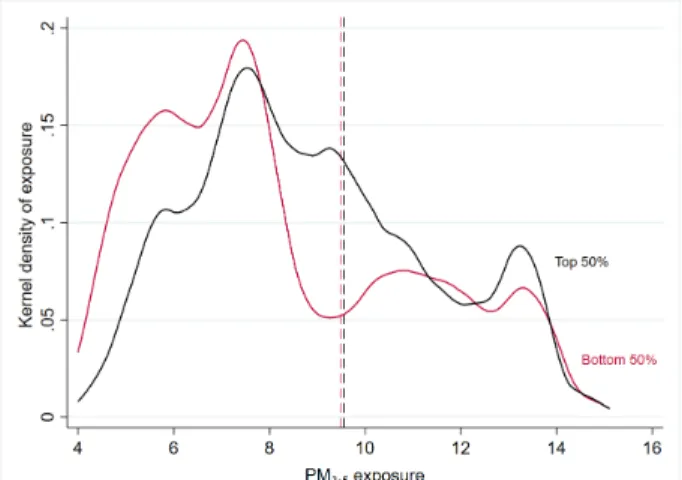
This small difference in average exposure between the two groups masks specific patterns, as shown in Figure 3. The latter displays the distribution of exposure to PM2.5 within the two halves

of the national distribution of IRIS (median) income. Given that the number of observations is identical between the two groups, I can directly interpret gaps in the probability density functions as an occurrence of over- or under-representation. It seems that one can split these two

distribu-tions into three parts. At “very low” levels of exposure, between 4 and 7 µg/m3, the bottom 50% of income is over-represented, in all likelihood due to the fact that rural areas usually combine low

income and low pollution levels. At middle-range levels (7-10 µg/m3), the top 50% of income is over-represented. Finally, focusing on levels of exposure above the WHO guideline of 10 µg/m3, the

top and bottom 50% are quite similarly represented, with a slightly higher proportion of top-50% neighbourhoods. This pattern is likely attributable to the characteristics of French urban areas:

Figure 3: Distribution of exposure to PM2.5, top and bottom 50% of income – 2016

Note: The dashed vertical lines represent the mean value of exposure for each group. The median level of income is equal toe20,252.

(17)

albeit different levels of residential segregation, statistically more polluted city centres and inner

suburbs usually compound both high- and very low-income neighbourhoods, and peri-urban areas are increasingly well-off (Aerts et al., 2015; Floch, 2014, 2017).

Figure 4 relies on a finer group definition: Figure 4a compares the distribution of exposure of

the top 10% to that of neighbourhoods between the 8th and the 9th decile of income, while Figure 4b compares the exposure of the bottom 10% to that of neighbourhoods between the 1stand the 2nd

decile of income. It appears that the likelihood of experiencing very high levels of exposure is indeed considerably higher for the top 10% IRIS than for any of the three other groups. On the other hand,

a large fraction of neighbourhoods whose income lies between the 8th and the 9th decile are exposed to PM2.5 levels that are below the national average of 9.54 µg/m3. The patterns of distribution of

exposure are very different in Figure 4b, which suggests that the neighbourhoods located below the 1st decile of IRIS-level income (i.e., whose median income is belowe16,162) are substantially more likely to be exposed to high PM_2.5 levels: 60% of these low-income neighbourhoods are above the

WHO standard, while, conversely, 80% of the neighbourhoods of the next 10% comply with this standard (see the CDFs in Appendix Figure 19). This is consistent with the fact that, in France in

2012, 65% of individuals living below the poverty line lived in large urban centres (INSEE’s grands pôles urbains), and 20% in the Paris urban area (Aerts et al., 2015).

Figure 4: Distribution of exposure to PM2.5 – 2016

(a) 8-9th _{decile and top 10%} _{(b) Bottom 10% and 1-2}nd _decile

Note: The 8th decile of income is equal to e23,627, and the 9th decile is equal toe26,286 (left). The 1st decile of income is equal toe16,162, and the 2nd decile of income is equal toe17,738 (right).

(18)

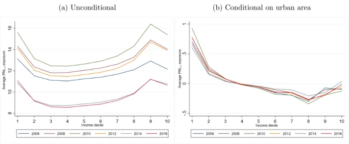
Figure 5a displays the unconditional average exposure to PM_2.5 as a function of a

neighbour-hood’s decile of income, for all even-numbered years of the study period, and rather corroborates previous evidence. As a consequence of the aforementioned phenomena relating income and location

in France, there appears to be a U-shaped relationship between unconditional average exposure and income. However, the average exposure of the top 10% of IRIS income is lower than that of those

located at the 9th decile of income, and similar to that of the bottom 10% of IRIS-level income. Conditioning PM_2.5 exposure on urban area yields a completely different story: within urban areas,

neighbourhoods with very low income are substantially more polluted than their wealthier coun-terparts. Average exposure roughly decreases with income up to the 7th decile, and then slightly

rises with income at the right end of the distribution. Notice also that conditionally on urban area, the exposure of neighbourhoods whose income lies between the 4th and the 9th decile is lower than

average, while the top 10% have average exposure.

Figure 5: Average exposure to PM2.5 based on (national-level) income decile

(a) Unconditional (b) Conditional on urban area

3.2 _{Fixed-effect models}

I provide a more formal analysis of the correlation between fine particulate matter exposure and neighbourhood income by running IRIS-level fixed-effect models. By doing so, I exploit the variation

in income and PM2.5 concentration within census blocks, and thus difference out the potentially

confounding effect of unobserved census block-level characteristics which could influence the location

(19)

characteristics (listed in Appendix Table 6), it remains that I do not observe the quality of the

amenities present within or in the vicinity of neighbourhoods. These are particularly important in this study due to the fact that households likely substitute away air quality for other amenities, such

as cultural facilities, schools or proximity to large business districts. Although not discussed, this omitted variable bias is present in any of the abovementioned cross-section analyses (e.g., Ouidir

et al., 2017; Zwickl et al., 2014) whose model identification relies on variations across study areas. The corresponding equation is the following:

ln(PMit) − ln(PMi) = α + βIN C(ln(INCit) − ln(INCi)) + βX(Xit− Xi) + λt+ (εit− εi) (1)

PM_2.5 exposure is right-skewed, so I take its natural logarithm in all regressions. ln(PM_it)

corre-sponds to the (log) average exposure in IRIS i, during year t. ln(INCit) is the median income of

IRIS i in year t. X_it includes the covariates taken from the list displayed in Table 6 in Appendix. I

include the share of inhabitants that undertook higher education, since more educated individuals may attach a higher value to air quality than less educated individuals, and thus hold a different

view of the trade-off between amenities and air pollution, which influences their residential choice. For similar reasons, I select the shares of population by occupation, divided in 8 categories (see

Appendix Table 6). Moreover, homeowners and subsidised housing tenants, i.e., those who live in HLM (Habitation à Loyer Modéré), may have more stringent residential mobility constraints than

tenants of privately owned dwellings, which would prevent them from leaving polluted areas. I also control for the share of dwellings that are not equipped with electric heating, since domestic

wood burning is one of the main sources of PM2.5 in France (Citepa, 2018), and similarly for the

share of households that own a car. The fractions of immigrants, of unemployed individuals, and

single-parent households are also used as measures of deprivation (Pornet et al., 2012). Finally, I cluster standard errors at the employment-zone level in order to account for autocorrelation within

employment zones, and weight regressions by population.

I take advantage of the panel structure of my data to deal with the omitted variable bias related to time-invariant unobserved IRIS-level characteristics, and I add year fixed effects in order to tackle

the impact of year-specific shocks that would impact both income and PM2.5 concentration, such

as a shock in economic activity. However, it is likely that there are remaining biases, meaning that

(20)

exists no time-varying unobserved heterogeneity across IRIS throughout the 2006-2016 time period,

since it was computationally inaccessible to introduce more than 400,000 time-varying fixed effects. Second, unlike an individual-level fixed-effect model, the models that I estimate do not fully tackle

the self-selection issue that is inherent to the study of environmental inequality. Indeed, they do not resolve the potential reverse causality of the pollution-income relationship,8 which opposes the

neighbourhood sorting hypothesis to the firm siting hypothesis. As a consequence, the test that I provide here boils down to looking at whether any of these two hypotheses, or a combination of the

two, may apply to France.

Table 1 shows the results associated with equation (1). The crude model with only IRIS fixed effects shows a strong negative correlation between IRIS median income and PM2.5exposure, and the

following ones as well, though it is less pronounced. In the preferred specification (Column (3)), in which I control for year fixed effects as well as neighbourhood characteristics, the estimates suggest that over the 2006-2016 period, a 1% positive deviation from a neighbourhood’s mean income is

associated with a decrease of .18% of its mean PM2.5 concentration, ceteris paribus. While these

models do not identify a causal impact, but a correlation net of the impact of certain variables,

they support the idea that, at the national scale, a higher neighbourhood income is associated with a lower exposure to PM_2.5. Therefore, these results do not contradict the Tiebout (1956)

sorting mechanism evoked in Banzhaf et al. (2019). As a clean environment can be considered as a luxury good, higher air quality may prop up rents and housing prices.9 As a direct consequence,

there may be a sorting phenomenon of households across income groups, even if households do not necessarily choose to migrate due to higher air pollution (Banzhaf and McCormick, 2012). These

results are also theoretically consistent with a theory of disproportionate siting by firms. However, this mechanism likely plays a less significant role in the case of fine particulate matter as compared

to other pollutants, since a bit less of a quarter of emissions are emitted by the manufacturing sector, while two thirds are from residential sources and transportation (Citepa, 2018). Finally,

this result may also be attributed to a combination of both processes of sorting and siting, through Coasian bargaining (Banzhaf et al., 2019). In any case, I only provide the first piece of evidence of

8

Lagged independent variables are not particularly helpful in this context, given the degree of inertia of the variable of interest between 2 subsequent years of observation at the IRIS level.

9_{To my knowledge, only two studies investigated this in France. Lavaine (2019) found evidence of a significant}

impact of air quality on housing prices in the highly polluted Dunkirk metropolitan area, while Le Boennec and Salladarré (2017) did only for specific types of households in the less polluted Nantes region. It may be hypothesised that the intensity of sorting dynamics could vary depending on the overall pollution level of an urban area.

(21)

Table 1: Fixed effect models – Partial results Variable (1) (2) (3) (Log) income -1.274 ∗∗∗ _-.212∗∗∗ _-.182∗∗∗ (.137) (.037) (.025) % Immigrants .143 ∗∗∗ (.025) % Higher education .141 ∗∗∗ (.039) % White-collar .258 ∗∗ (.105)

% Inactive excl. retired .113

∗∗ (.054) % Unemployed -.119 (.105) % Social housing .051 (.054) Intercept 15.062 ∗∗∗ _4.542∗∗∗ _4.061∗∗∗ (1.357) (.368) (.344)

Year fixed effects X X

R2 within 0.11 0.78 0.79

R2 between 0.02 0.01 0.21

R2 overall 0.01 0.18 0.37

# Observations 453,386 453,386 453,306

# Groups 42,832 42,832 42,825

Standard errors clustered at the employment-zone level in parentheses. ∗: 10% level,∗∗: 5% level,∗∗∗: 1% level.

this national-level correlation: further research based on individual-level data would allow to better understand the mechanisms behind this inequality.

Finally, paying specific attention to other neighbourhood characteristics, the results also suggest that there is a positive correlation between the share of immigrants and exposure to fine particulate

matter, even after controlling for income. This cannot be attributed to the fact that a great fraction of immigrants are gathered in specific neighbourhoods of large metropolitan areas, since I control for

IRIS-level unobserved heterogeneity. Therefore, there might also be an ethnic gap in exposure to fine particulate matter in France, as observed in the US (Currie et al., 2020; Kravitz-Wirtz et al., 2016).

(22)

The positive link between PM_2.5 concentration and the shares of highly educated individuals, of

white-collar workers, and inactive individuals – the latter being mostly students, since the category excludes retirees – is consistent with the fact that these populations tend to concentrate in urban

centres. On the other hand, there is no significant relationship between unemployment share and PM_2.5 level, likely due to the fact that unemployment is not only high in polluted former industrial

areas, but also in cleaner rural ones. The same observation applies to the share of subsidised housing, for which I find no significant result. This may also stem from the fact that although there

are significant variations in the share of social housing across IRIS, there may not be large enough variations within IRIS for any significant difference to be identified. The remainder of the estimates

are provided in Appendix Table 8, and the coefficients all appear consistent with theory.

3.3 _{Robustness to spatial autocorrelation}

Tobler’s (1970) first law of geography states that “everything is related to everything else, but near things are more related than distant things”. Indeed, spatial autocorrelation is likely to be of

par-ticular concern when one examines the relationship between income and access to clean air. Air pollution levels are spatially correlated by construction, and income does not verify complete spatial

randomness (CSR) either: in France, residential income segregation is less pronounced than in the US (Quillian and Lagrange, 2016), but tends to increase (Beaubrun-Diant and Maury, 2020). In

Sec-tion 3.2, standard errors are clustered at the employment-zone level, which means that correlaSec-tion within employment zones is allowed for. This implies that spatial correlation is modelled discretely,

since it is designed to follow employment zone boundaries. Pollution, however, is distributed con-tinuously across space. As a consequence, pollution levels on either side of an employment zone

boundary are thus as likely to be correlated as pollution levels of two IRIS located within the same zone. This argument also holds for other neighbourhood characteristics. Hence, the residuals of

equation (1) are most likely not independently distributed. Moreover, failing to take spatial au-tocorrelation into account amounts to have an artificially lower variance in observations, and thus

artificially lower standard errors, thus inflating the risk of Type-I error.

To my knowledge, despite the importance of the issue in this setting, environmental inequality studies performed by economists generally lack concern for spatial autocorrelation. In a related

study, Lavaine (2015) does use Driscoll-Kraay standard errors, which are robust to cross-sectional correlation, in some specifications. Nonetheless, a number of studies do not mention it (e.g., Currie

(23)

et al., 2020; Muller et al., 2018; Voorheis, 2017; Zwickl et al., 2014). Concern for spatial

autocor-relation is however more common within the Public Health literature on the topic: some highlight the consequences of failing to account for it (e.g., Havard et al., 2009), and among those mentioned

in Section 1.2, a large part uses specifically designed spatial models.

Some adopt spatial lag models, a specific version of Spatial Autoregressive (SAR) models (Havard

et al., 2009; Verbeek, 2019). Spatial lag models treat spatial dependence between observations as substance, as opposed to a disturbance. They assume that the value taken by the dependent

variable in each zone both affects and is affected by the values taken by the dependent variable in the neighbouring zones, which is exactly what one may expect when the outcome variable is

pollution exposure. With W a weighting matrix, a basic spatial lag model may be thus written Y = Xβ + ρW Y + ε. The choice of the form of the spatial weighting matrix W is however arbitrary,

as it amounts to making parametric assumptions about the behaviour of spatial autocorrelation. Finally, misspecifying the spatial weight matrix can introduce large biases in the final estimates (Anselin, 2002; Lam and Souza, 2014).

An appealing solution is thus to opt for a non-parametric approach to account for spatial

auto-correlation. Specifically, I use a Generalised Additive Model (GAM). These are Generalised Linear Models (GLM) to which one adds a smoothing function of at least some covariates. As such, while

they were not designed as spatial models to begin with, they allow to add a non-parametric function of geographic coordinates to account for neighbourhood location as a possible predictor of PM_2.5.

Unlike spatial lag models, GAM thus do not impose parametric assumptions on the form of spatial autocorrelation. Hence, they were used to model spatial autocorrelation in studies of interregional

knowledge spillovers (Guastella and Van Oort, 2015), interregional risk sharing (Basile and Girardi, 2010) or hedonic house pricing (Helbich et al., 2014; Von Graevenitz and Panduro, 2015). They

have also been used in few environmental justice studies (Brochu et al., 2011; Padilla et al., 2014). Thus, I add the latitude y_i and longitude x_i of the centroid of IRIS i as a smoothed term

s(xi, yi) to equation (1).10 s(·) is a thin plate regression spline, which does not require to specify

knots. The most widespread approach used to estimate GAM is the backfitting algorithm of Hastie

and Tibshirani (1990) but, in practice, it implies that one must select the degree of smoothness of the term s(x_i, yi). Selecting the degree of smoothness amounts to selecting the span size, i.e., the

10_{Modelling spatial autocorrelation this way is thus akin to tackling the omitted variable bias arising from the fact}

(24)

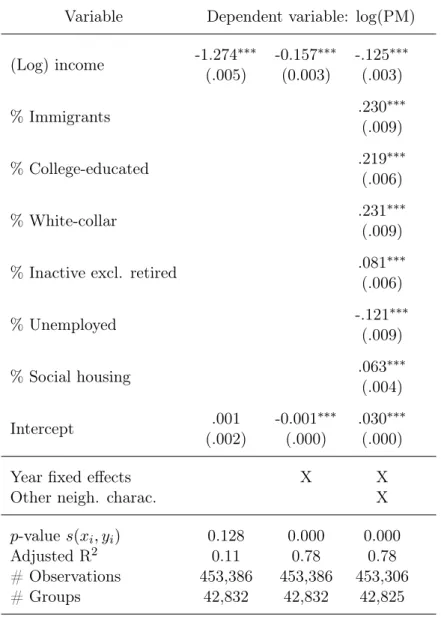
Table 2: Fixed-effect generalised additive models – Partial results

Variable Dependent variable: log(PM)

(Log) income -1.274 ∗∗∗ _-0.157∗∗∗ _-.125∗∗∗ (.005) (0.003) (.003) % Immigrants .230 ∗∗∗ (.009) % College-educated .219 ∗∗∗ (.006) % White-collar .231 ∗∗∗ (.009)

% Inactive excl. retired .081

∗∗∗ (.006) % Unemployed -.121 ∗∗∗ (.009) % Social housing .063 ∗∗∗ (.004) Intercept .001 -0.001 ∗∗∗ _.030∗∗∗ (.002) (.000) (.000)

Year fixed effects X X

Other neigh. charac. X

p-value s(xi, yi) 0.128 0.000 0.000

Adjusted R2 0.11 0.78 0.78

# Observations 453,386 453,386 453,306

# Groups 42,832 42,832 42,825

Standard errors clustered at the employment-zone level in parentheses. ∗: 10% level,∗∗: 5% level,∗∗∗: 1% level.

number of IRIS in the vicinity of IRIS i whose outcomes are likely correlated with these of IRIS i, and thus boils down to a bias-efficiency trade-off. In order not to resort to arbitrary choices, I rely

on more recent advances in research on GAM, which led to the development of a new estimation technique that singles out the degree of smoothness in an automatic and integrated fashion. Hence,

the optimal smoothing parameter is obtained via generalised cross-validation (Wood, 2017).

The results that mirror those of Table 1 are displayed in Table 2, and the full set of estimates is

provided in Appendix Table 9. The approximate p-value of the smoothing term s(xi, yi) is highly

(25)

Another striking element is the fact that, for any specification, the intercept is substantially smaller

than before, and the adjusted R2 substantially higher than before, since neighbourhood location likely explains a great fraction of PM_2.5 variation. Although omitting to allow for spatial

autocor-relation theoretically shrinks standard errors, significance levels are much higher than in previous models. It appears that as I net spatial autocorrelation out, the pollution-income relationship

weak-ens, although the estimates are not significantly different from before: a 1% increase from the IRIS mean median income is associated with a .125% reduction in mean PM_2.5 exposure. This

sup-ports the idea that the spatial dimension does not attenuate nor invalidate the relationship between income and environmental hazard in the case of PM2.5 exposure.

Notwithstanding, the positive relationship between PM2.5 concentration and the share of

im-migrants is significantly stronger than under the previous specification at the 5% level, with an

estimate of .230 as opposed to .143. Equation (1) considered IRIS as independent of each other, but diagnosed a positive correlation between PM2.5concentration and share of immigrants within census

blocks. There is a positive spatial autocorrelation of both pollution and the share of immigrants

across these blocks, which attenuates with distance. Consequently, controlling for the longitude and latitude of a census block that has a high (resp., low) pollution level accounts for the fact that its

neighbours also have a high (resp., low) pollution level, and thus a likely high (resp., low) share of immigrants. In other words, allowing for spatial autocorrelation places IRIS back into their

rela-tive location, thus creating “clusters” that combine high values of PM2.5 and share of immigrants

together, medium values together, and low values together, which implies that the correlation is

indeed higher than what simple FE models estimated. On the other hand, as aforementioned, the estimate associated with income is lower in absolute terms than previously evaluated, with an

esti-mated coefficient of -.125 against -.182. These two findings can thus seem conflicting at first sight, but can be reconciled, since they imply that, for a given degree of spatial smoothing, income is

distributed more uniformly across space than the share of immigrants. Indeed, in France, ethnic segregation measures provided by, e.g., Gobillon and Selod (2007), Préteceille (2011) or Safi (2009),

are higher than income segregation measures (Floch, 2017; Quillian and Lagrange, 2016).

The estimates associated with the shares of college-educated individuals, white-collar workers

and inactive inhabitants, and those only presented in Appendix Table 9, are qualitatively and quan-titatively similar to the previous ones, making them robust to accounting for spatial autocorrelation.

Finally, the estimates for the unemployment share and the social housing share are now statistically significant, which may also be attributed to segregation.

(26)

3.4 _{Evolution in exposure and longitudinal inequality}

3.4.1 _{Graphical evidence}

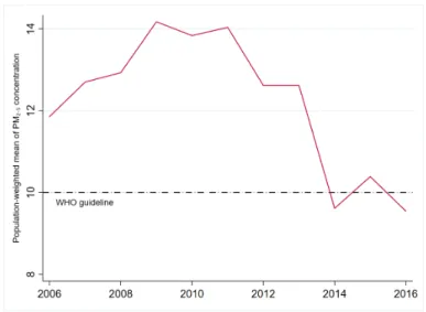
Figure 6 displays the evolution of average exposure to fine particulate matter in metropolitan France

throughout the study period. According to this figure, average exposure increased from 11.85 µg/m3 in 2006 to around 14 µg/m3 for 2009-2011, before falling to 9.54 µg/m3 in 2016. Hence, for years

2014 and 2016, according to matched ACAG and INSEE data, exposure seems to be line with the World Health Organisation (WHO) guideline of 10 µg/m3, on average. Average exposure fell by

4.63 µg/m3, or 32.7%, between the peak year 2009 and 2016, a decrease similar to the United States’ in the 2000-2014 period (Currie et al., 2020; Voorheis, 2017).

Figure 6: Evolution of average exposure to PM_2.5 – 2006-2016

However, this national average masks some considerable spatial disparities in the evolution of

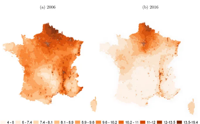
fine particulate matter concentration. Figure 7 shows two years of this concentration for metropoli-tan France, by decile of the total distribution across these two years. In 2006, the least exposed areas

were Massif Central, the Pyrénées, the southern part of the Bay of Biscay and the tip of Brittany, and remain so. More specifically, PM2.5 concentration was already very low in Massif Central, and

did not significantly decrease, while it did in the last three regions. On the other hand, the northern part of the country, the Paris region and the Rhône Valley, which were located in the top 30% of the distribution in 2006, stayed at this position in 2016. This implies that while pollution was already

high in these areas, and particularly much higher than the WHO guideline, they remained at the top of the cross-year pollution distribution, while the rest of the country moved down. Taken

(27)

to-Figure 7: Exposure to PM2.5 by decile

(a) 2006 (b) 2016

gether with the map of Figure 2b, this does not allow to draw clear-cut conclusions on longitudinal patterns of inequality: while the low-income northern départements remained polluted, high-income

ones like Rhône or Seine-et-Marne also did.

As a first piece of evidence on longitudinal environmental inequality, I switch back to the income group definitions of Section 3.1. Figure 8a distinguishes between the top and the bottom 50% of the income distribution, and shows that the top 50% of income appears to be consistently more exposed

to PM2.5 than the bottom 50%, experiencing a larger increase in exposure during the 2006-2011

period, and a rather similar overall decrease up to 2016. The fact that urban areas concentrate both

a high level of PM2.5 concentration, a high proportion of individuals, and a relatively high level of

income surely can explain a large part of the gap that we observe in this figure. However, patterns

are rather different when looking at the 4 group definitions also used in Section 3.1, namely the bottom and top 10% of income, and areas located between the 1stand the 2nddecile, and the 8thand

the 9th decile. The gap between the latter remains quite constant along the years. However, while they had roughly equal average levels of exposure during the 2008-2013 period, a gap in exposure

(28)

Figure 8: Evolution of average exposure to PM2.5 in different income groups – 2006-2016

(a) Top 50% vs Bottom 50% (b) Two highest and lowest deciles

may be arising between the neighbourhoods at the top and those at the bottom 10% of income, at the favour of the top 10%. This will be a trend to pay attention to in upcoming years.

Moreover, these results are obtained on the basis of varying ranks in the income distribution. A

small counterfactual exercise can highlight the potential role of mobility. Indeed, one can compute the average exposure of neighbourhoods in 2016 using their 2006 rank, and compare it to the actual

average. With this definition, the average of exposure of the bottom 10% of 2016 in 2016 is 11.30 µg/m3, but that of the bottom 10% of 2006 in 2016 would have been 11.08 µg/m3, holding the ranks

fixed. On the other end of the spectrum, the 2016 top 10%’s average exposure is equal to 10.86 µg/m3, while it should have been 11.01 µg/m3 holding the ranks fixed. As such, the bottom 10% of

2016 is more exposed than the 2006 bottom 10% would have been, and the reverse holds for the top 10%. This implies that neighbourhoods that are “new” to the bottom 10% are more polluted than

those that “left” the bottom 10%, and that neighbourhoods that are “new” to the top 10% are less polluted than those that “left” the top 10%. Such a fact is consistent with relative mobility patterns

that would occur due to the neighbourhood sorting mechanisms, where higher-income (resp., lower-income) individuals would self-select into cleaner (resp., more polluted) neighbourhoods, be it due

to pollution-related out-migration or to market forces (Banzhaf and McCormick, 2012; Banzhaf et al., 2019). Individual data would be needed to formally test these hypotheses.

(29)

3.4.2 _{Pollution-reduction profiles}

In order to study longitudinal inequality in exposure to fine particulate matter, I proceed to compute

pollution-reduction profiles, following Voorheis (2017). Voorheis argues that, although there is a sizeable body of literature on the cross-sectional measurement of environmental inequality in the US,

much less is known about longitudinal environmental inequality. As such, he adapts a method used in the literature on intra-generational mobility and first proposed by Jenkins and Van Kerm (2006),

called income-reduction profiles, to pollution exposure. The resulting pollution-reduction profiles (PRP) allow to capture both vertical equity concerns (i.e., how PM_2.5 exposure varies across

ini-tial ranks of exposure) and horizontal equity concerns (i.e., how PM2.5 exposure varies across initial

ranks of income). Both types of PRP are also computed both in absolute terms, using the difference

between exposure in year t + x and exposure in year t, and in relative terms, using the difference between the logarithm of exposure in year t + x and that of year t. As shown in Figure 6, average

exposure increased between 2006 and 2011, and decreased ever since. This framework thus allows to visualise the distributional impacts of the 2006-2011 air quality deterioration and the 2011-2016

(and overall) air quality improvement. All PRP are obtained by fitting a thin plate regression spline.

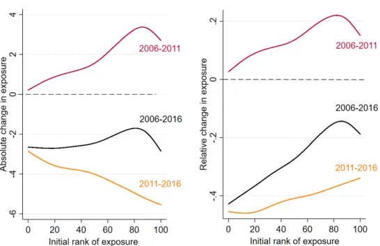
Figure 9 (resp., Figure 10) shows the vertical (resp., horizontal) equity profiles, with absolute

changes in exposure on the left-hand side and relative changes in exposure on the right-hand side. I begin by looking at the change in exposure as a function of a census block’s initial rank in the

dis-tribution of exposure. Between 2006 and 2016, regardless of their initial level of exposure to PM2.5,

on average, IRIS benefitted from overall quite comparable decreases in absolute terms, between

-1.7 µg/m3 and -2.8 µg/m3. However, this implies that, in relative terms, census blocks that were initially less exposed to PM_2.5 benefitted from larger improvements than those who were initially

more exposed. Distinguishing between the two phases of the study period, the graph suggests that initially disadvantaged census blocks experienced a higher increase in exposure between 2006 and

2011, and a smaller relative decrease in exposure between 2011 and 2016, compared to their initially less exposed counterparts. In particular, neighbourhoods at the 10th percentile of initial exposure

received a 40% decrease in exposure, while those at the 90th percentile received a 14% decrease. In short, the vertical equity measures suggest that both the rise and the fall in PM_2.5 concentration

(30)

Figure 9: Pollution-reduction profiles – Vertical equity

Note: The initial rank of exposure is the rank in the distribution of IRIS exposure to PM2.5 in 2006.

This is consistent with what Figure 6 shows at a larger geographical scale: while PM2.5

con-centration decreased throughout metropolitan France, regions that were initially the most polluted,

such as Hauts-de-France and Île-de-France, did not experience larger relative decreases than others. This may partly be attributed to relatively smaller decreases in emissions due to less effective

poli-cies, but another potential explanation for this may be that fine particulate matter concentration did not decrease more in initially more polluted areas because a potentially significant part of these

particles is imported. Indeed, PM2.5 can travel long distances, which implies that a potentially

non-negligible part of neighbourhoods’ observed concentration is not due to domestic emissions.

For instance, in Île-de-France in 2010, it was estimated that 39% to 68% of their observed quantity was produced outside the region (Airparif, 2011).

Turning to the horizontal equity measures of Figure 10, the first finding is that, similarly to

ver-tical equity measures, absolute changes in exposure over the whole study period were rather uniform across the initial income distribution, with a 2 µg/m3 decline up to the 8th decile, and an average

decrease of 1.8 µg/m3 for the top 10% of income. However, in relative terms, the bottom decile of initial income, i.e. neighbourhoods with a median income of e14,300 in 2006,11 received a 20%

11

(31)

decrease in exposure, while those at the 4th decile (e17,360), received the largest relative decrease of 28%. Neighbourhoods of the top 10% of income (whose 2006 income is abovee24,000) benefitted from the smallest relative improvement, with a 17% average decrease in PM_2.5 concentration. To

summarise, in relative terms, it appears that the pollution-reduction profile is U-shaped, with air quality improvements accruing to a greater extent to neighbourhoods located in the middle 60%,

while those at the top and the bottom of the initial income distribution experienced significantly smaller relative decreases. Splitting the study period into the two phases studied above, it appears

that the bottom 20% and the top 20% of income not only experienced the largest (relative or abso-lute) increase in exposure between 2006 and 2011, but also slightly smaller relative decreases after

2011. Taken together with the evidence in Figure 9 and Section 3.1, these patterns are consistent with an overall improvement of fine particulate matter pollution throughout the country, which,

however, favoured municipalities and neighbourhoods that combine intermediate income and com-paratively low pollution levels. This implies that although overall PM2.5 exposure underwent a

substantial drop during the study period, inequality in exposure intensified.

Figure 10: Pollution-reduction profiles – Horizontal equity

(32)

4 _{Role of Plans de Protection de l’Atmosphère}

In France, part of the regulation of air quality occurs at the level of urban areas, through mandatory Plans de Protection de l’Atmosphère. As a consequence of a 2008 EU Directive that incorporated

fine particulate matter as a newly regulated pollutant, urban areas were required to revise their schemes, so as to include measures aimed at reducing PM_2.5 concentration. Using an event-study

design, this section investigates whether this change in policy helped reduce inequality in exposure to my pollutant of interest.

4.1 _Context

The EU Directive 2008/50/EC on air quality, also named Directive on ambient air quality and cleaner air for Europe, includes 4 elements. First, it merged the majority of existing legislation on

air quality into a single directive,12without any change in existing objectives. Second, it allowed for time extensions for compliance to EU standards regarding the concentration of particulate matter

(PM10), benzene, and nitrogen dioxide (NO2), up to 2015. Third, it gives the opportunity for

Member States to deduct emissions caused by natural sources, such as those emitted through forest

fires, when assessing compliance to EU limit values of regulated pollutants. The fourth and final element of the Directive is of particular interest: it established that annual concentration in PM2.5

has to be lower than 25 µg/m3 _{by the 1}st _{of January, 2015. In terms of exposure, the Commission}

chose to refer to a three-year annual average exposure (AEI, for Average Exposure Indicator), which must be lower than 20 µg/m3_{. In France, the AEI is computed using monitor data of 49 urban}

areas. This became legally binding in 2015, i.e., starting for years 2013-2015. The Directive was translated into French law, and thus integrated into the Code de l’Environnement, by decree, on

the 21st of October, 2010.13

The LAURE (Law on Air and Rational Use of Energy) of 1996 already compelled urban areas

of more than 250,000 inhabitants to implement an Atmosphere Protection Plan (PPA, for Plan de Protection de l’Atmosphère), which, among other requirements, has to comprise a precise agenda of

measures taken by local authorities so as to meet air quality standards.14 The 2008 EU Directive

12

The Directive 2008/50/EC merged all existing legislation on outdoor air quality, apart from the Fourth Daughter Directive 2004/107/EC, which regulates the concentration of metals, such as mercury and nickel, in ambient air.

13

Said decree is available online at https://www.legifrance.gouv.fr/affichTexte.do?cidTexte= JORFTEXT000022941254&categorieLien=id.

14

In addition to the action plan, the elements that a PPA must contain are: a) an inventory of emissions of atmospheric pollutants b) an evaluation of air quality c) a description of the sanitary impacts of air pollution d) an evaluation of the measures taken, in the form of scenarios.