Amplitude equations for Rayleigh-Be´nard convective rolls far from threshold
P. C. Dauby*and Th. DesaiveUniversite´ de Lie`ge, Institut de Physique B5, B-4000 Lie`ge 1, Belgium J. Bragard
Department of Physics and Center for Interdisciplinary Research on Complex Systems, Northeastern University, Boston, Massachusetts 02115
P. Cerisier
IUSTI, UMR CNRS 6595, Universite´ de Provence, Technopoˆle Chaˆteau-Gombert, Rue E. Fermi 5, F-13453 Marseille Cedex 13, France 共Received 13 February 2001; published 9 November 2001兲
An extension of the amplitude method is proposed. An iterative algorithm is developed to build an amplitude equation model that is shown to provide precise quantitative results even far from the linear instability thresh-old. The method is applied to the study of stationary Rayleigh-Be´nard thermoconvective rolls in the nonlinear regime. In particular, the generation of second and third spatial harmonics is analyzed. Comparison with experimental results and direct numerical calculations is also made and a very good agreement is found. DOI: 10.1103/PhysRevE.64.066301 PACS number共s兲: 47.20.Bp, 05.45.⫺a, 44.25.⫹f, 47.27.Te
I. INTRODUCTION
Rayleigh-Be´nard共RB兲 convection 关1,2兴 is an illuminating example of pattern formation outside of equilibrium. Numer-ous studies have been devoted to this system. Some of them are concerned with the nonlinear competition between differ-ent structures that develop above the linear convective threshold. For instance, the stability domains of rolls, hexa-gons, or square cells have been determined in terms of the different parameters of the system 关3–5兴. The transition to more complex, nonstationary, behaviors has also been ana-lyzed 关6兴. Interesting general references to the RB problem may be found, for instance, in the books by Koschmieder关1兴 and by Colinet et al. 关2兴.
Navier-Stokes equations, and, more generally, the equa-tions of continuum mechanics are nonlinear. More precisely, in the simplest cases, the nonlinearities are quadratic and originate in the advective terms of the material time deriva-tives. For this reason, when a spatial structure appears in the solution of these equations, its second-order harmonics are directly excited through the quadratic terms and may influ-ence the observed pattern. An interesting illustration of the influence of the second-order harmonics has been recently presented by Regnier et al. 关5兴 who examined the interface deformations of an hexagonal pattern in coupled gravity-driven and capillary thermoconvection. They showed that when the depth of the fluid layer is such that the deforma-tions of the upper free surface due to gravity and due to capillarity exactly compensate for the linearly unstable mode, the interface relief in the nonlinear regime is deter-mined by the second-order harmonics only共‘‘hybrid’’ relief兲. One motivation of the present work is the experimental evidence of the appearance of not only second-, but also third-order harmonics in a thermoconvective roll pattern in the RB problem. This problem has already been approached
by several authors in the past共see, for instance, 关7兴 and ref-erences therein兲. In 关8兴, experimental results are reported and a perturbation analysis limited to third-order terms and based on the Malkus-Veronis approach 关9,10兴 is presented and compared with experiments. Pure numerical calculations关11兴 and a double Fourier expansion in x and z combined with a Galerkin method 关7兴 are also shown to display the appear-ance of the second- and third-order harmonics of the basic sine roll pattern.
In this paper, we propose an extension of the amplitude method used in many nonlinear studies on thermoconvection 共see 关2兴 and references therein兲. From a theoretical point of view, the original amplitude method is valid only asymptoti-cally close to the linear stability limit. Unfortunately, this method has sometimes been used to analyze nonlinear re-gimes that are not close to the threshold. For instance, the depth of the subcritical convection domain in Marangoni convection and the transitions between rolls, hexagonal cells, and square patterns were determined in this context 关3–5兴. The value of the control parameter corresponding to these bifurcations is not always small, which makes these results questionable, from a quantitative, but also from a qualitative, point a view.
In this paper, we develop an extended amplitude formal-ism to allow a rigorous analysis of convection further from the linear threshold. For simplicity and clarity, the formal-ism, which is based on an iterative algorithm, is presented here through a detailed analysis of Rayleigh-Be´nard thermo-convective rolls in the nonlinear regime. More precisely, we show that the extended method permits us to account in an easy way for the experimental observations of the second and third spatial harmonics. The validity of the method far from the threshold is checked by confronting it to experi-mental data and also direct numerical simulations.
Our experimental set-up is described in details in关12兴. Let us summarize the description of the apparatus 共Fig. 1兲. A finite rectangular container with dimensions 12⫻3⫻1 cm3 is filled up with a Rhodorsil 47V100 silicone oil and heated *Electronic address: [email protected]
from below. The upper and lower boundary of the fluid are two horizontal glass plates with a thickness of 0.3 cm. By measuring the deflection of a laser beam shining through the fluid, the overall horizontal temperature gradient is deter-mined 关12兴. The velocity field is also measured using PIV. For a relative distance to the linear convective threshold slightly larger than 1, second- and third-order harmonics clearly appear in the horizontal temperature gradient and ve-locity field.
In Sec. II, the basic governing equations for the RB prob-lem are recalled and the classic nonlinear amplitude method is briefly described. Section III contains a qualitative expla-nation of the presence of secondary harmonics based on an amplitude model with only four modes. In Sec. IV, we present the extended amplitude method, which is the main result of the paper. It consists in a precise strategy to build an amplitude model valid even far from threshold. We compare the solution given by this model with direct numerical cal-culations. We show that in the specific case of RB convec-tion, a model with 11 amplitude equations gives very good quantitative agreement with numerics. We present our ex-perimental results in Sec. V and again compare these results with the solution of our model. Conclusions are drawn in the last section.
II. BASIC EQUATIONS AND BASIS OF THE NONLINEAR METHOD
Let us consider, for simplicity, a horizontally infinite fluid layer that is contained between two rigid horizontal bound-aries. The equations for this system are well known 关1,2兴. When the Boussinesq hypotheses hold, the perturbations with respect to the conductive solution obey the following set of partial differential equations:
“•u⫽0, 共1兲
Pr⫺1关tu⫹共u•“兲u兴⫽⫺“p⫹“2u⫹Ra Tez, 共2兲
tT⫹u•“T⫺w⫽“
2T. 共3兲
We have chosen the vertical z axis in the direction opposite to gravity. The equations are written in a dimensionless form with lengths scaled by the thickness d of the liquid layer. The time scale is d2/, with the heat diffusivity of the liquid. The velocity is scaled by /d and the temperature scale is chosen as d, where is the vertical temperature gradient that would exist in a purely conductive state. Symbols u ⫽(u,v,w), p, and T represent the dimensionless perturba-tions共with respect to the conductive solution兲 of the velocity, pressure, and temperature fields. The Rayleigh and Prandtl numbers Ra and Pr are defined as
Ra⫽g␣d 4
, 共4兲
Pr⫽
, 共5兲
where and ␣ are the liquid kinematic viscosity and the coefficient of thermal expansion, respectively.
The boundary conditions for the velocity perturbations at the bottom (z⫽0) and at the top (z⫽1) of the layer express the no-slip condition along the horizontal plates. For the tem-perature perturbations, a general Biot condition describes the heat exchanges through the boundaries. The corresponding equations are
u⫽0 at z⫽0 and at z⫽1, 共6兲
⫺Tz⫹Bi0T⫽0 at z⫽0, 共7兲
T
z⫹Bi1T⫽0 at z⫽1, 共8兲
where Bi0 and Bi1 denote the Biot numbers at the bottom and the top of the layer, respectively. In the experiments that we are considering in the present paper, these Biot numbers are equal since the glass plates at z⫽0 and z⫽1 are the same. The value Bi⫽46 is determined by using the expres-sion 关13兴 Bi⫽(wall/)关kc/tanh(kcdwall/d)兴 where wall ⫽1.74 Wm⫺1K⫺1 and dwall⫽0.3 cm are the heat conduc-tivity and thickness of the glass plates, while ⫽0.16 Wm⫺1K⫺1 is the heat conductivity of the silicone oil. The corresponding dimensionless critical wave number and Rayleigh numbers are given by kc⫽3.07 and Rac ⫽1653, respectively 共a standard spectral-tau method 关14,15兴 was used for the calculations of the critical parameters兲.
The starting point of our nonlinear method is the ampli-tude method that has been described in details, for instance, in关3,2兴. Two-dimensional rolls are the only convective pat-tern observed in the present experiments, therefore, the gen-eral three-dimensional method is simplified here into its two-dimensional共2D兲 counterpart. Let us recall the main steps of the method. First, the Rayleigh number is fixed to its critical value Racand the eigenmodes of the linearized equations are numerically determined by a spectral tau method, with the growth rate p of the perturbations as eigenvalue parameter. Using complex notations, the 2D eigenfunctions are
uk, p⫽Up共z兲exp共ikx兲exp共pt兲, 共9兲 Tk, p⫽p共z兲exp共ikx兲exp共pt兲, 共10兲 where k is the horizontal wave number and x the horizontal coordinate. It is important to note that for each value of k, an infinite set of eigenvalues exists for the growth rate, with corresponding vertical eigenfunctions Up(z) and p(z) for the velocity and temperature perturbations. The maximum value of the growth rate is zero and corresponds to a wave number equal to the critical value kc. The index p runs from FIG. 1. Sketch of the experimental setup
one to infinity and numbers the negative growth rates, which are assumed to be ordered in such a way that the real part of
p decreases with p共for k⫽kc, one has1⫽0兲. The eigen-modes are normalized in such a way that the maximum value of the modulus ofp(z) is equal to 1.
The solution of the nonlinear equations is then expressed as the following series depending on the eigenmodes (uP,TP):
冉
u T冊
⫽兺
AP共t兲冉
uP Rac Ra TP冊
⫹c.c. 共11兲 where P is written for k, p, and the AP(t) are the complex time-dependent amplitudes. It is worth emphasizing that the spatial functions used in this decomposition are not exactly the eigenmodes of the physical problem, due to the rescaling factor Rac/Ra. However, for each value of Ra, these func-tions uP and 共Rac/Ra)TP may be considered as the eigen-modes of a ‘‘mathematical’’ eigenvalue problem, which is easily obtained from the original problem by letting this fac-tor explicitly appear. These spatial modes may thus be con-sidered as independent. It may also be checked that the ad-joint eigenmodes of this problem are given by (uP쐓,(Ra/Rac)TP쐓), where the (u쐓P,TP쐓) are the adjoint eigen-modes of the original problem. From a more physical point of view, the introduction of the rescaling factor Rac/Ra in Eq.共11兲 may be justified by noting that the temperature scale used in Eqs. 共1兲–共3兲 isd while the ‘‘critical scale’’cd is used to determine the eigenmodes 共10兲. When the unknown fields are written under the form共11兲, the incompressibility Eq. 共1兲 and the boundary conditions 共6兲–共8兲 are automati-cally satisfied. The series 共11兲 is then introduced in Eqs. 共2兲–共3兲, which are then projected on the adjoint eigenfunc-tions of the ‘‘mathematical’’ problem introduced above. The momentum equation is thus multiplied by u쐓P, the velocity field of the adjoint eigenvalue problem and the energy equa-tion is multiplied by (Ra /Rac)TP쐓, with TP쐓 the temperature field of the adjoint eigenvalue problem. Both relations are added and integrated over the fluid volume. When the bior-thogonality relations between the solutions of the eigenvalue problem and its adjoint are used, together with the incom-pressibility condition and the boundary conditions, we get the following evolution equations for the amplitudes:dAP
dt ⫽PAP⫹⑀
兺
QMPQAQ⫹
兺
Q,L
NPQLAQAL. 共12兲
In this equation,⑀⫽(Ra⫺Rac)/Racis the relative distance to the threshold and the matrices M and N are given by
MPQ⫽
具
P 쐓w Q典
具
P쐓P⫹Pr⫺1uP쐓•uP典
, 共13兲 NPQL⫽⫺具
P 쐓共uQ•ⵜL兲⫹Pr⫺1u P 쐓•关共uQ•ⵜ兲uL兴典
具
P쐓P⫹Pr⫺1uP쐓•uP典
, 共14兲where the angular bracket is used to denote integration over the fluid volume.
Using a slaving principle关16,17兴, the infinite dimensional set of Eqs. 共12兲 may be reduced to a finite number of ordi-nary differential equations for the amplitudes of the most unstable modes of convection. The procedure leading to this reduced system may be briefly summarized as follows. First, the infinite number of eigenmodes is split into two catego-ries. The ‘‘basic’’ modes are the most unstable modes, with the real part of the growth rates close to zero while the ‘‘slaved’’ or ‘‘stable’’ modes are quite damped, due to quite negative values for Re(P). These slaved modes are present in the solution only as the quadratic response to the nonlinear growth of the basic modes above the threshold and their own dynamics may be neglected. For this reason, the time deriva-tive is set to zero in the evolution Eqs. 共12兲 for their ampli-tudes. This results in an algebraic relation between the basic and slaved amplitudes. When the amplitudes of the slaved modes are small with respect to the basic ones, the quadratic terms of these algebraic equations containing only damped modes may be neglected and the following expression of the slaved amplitudes in terms of the basic ones may easily be deduced:
APs⫽⫺ 1
Ps
兺
Q,LNPsQLAQAL, 共15兲
where the subindex s indicates that a slaved mode is consid-ered. In the right-hand side共r.h.s.兲 of Eq. 共15兲, the indices Q and L refer to basic modes only. Note that this relation, based on the smallness of APs, is always correct close to the thresh-old where the amplitudes of the basic modes can be assumed sufficiently small 共at least when the bifurcation is supercriti-cal, which is actually the case for rolls兲.
Expressions 共15兲 for the amplitudes of the slaved modes may then be introduced in the evolution Eqs. 共12兲 for the basic modes. If terms of order higher than three are ne-glected, the following final ‘‘amplitude equations’’ for the amplitudes of the basic modes are obtained:
dAP dt ⫽PAP⫹⑀
兺
Q MPQAQ⫹兺
Q,L NPQLAQAL ⫹兺
Q,L,R TPQLRAQALAR. 共16兲In this relation, all amplitudes and indices correspond to ba-sic modes only and the definition of the matrix T is easily deduced from the context. Note also that in practice only a finite number of slaved modes is considered to deduce Eq. 共16兲. Equations 共15兲 show that the amplitudes of the slaved modes decrease with p since the modulus of the growth rate increases with p. In the RB problem, the number Nsl(k) of slaved modes that are taken into account for each value of k is limited to four or five, which is sufficient to ensure con-vergence of the coefficients of the amplitude equations, as shown in关3兴 and checked again in this paper.
To finish this section, let us recall that the Eqs. 共16兲 should be considered as a valid model for the nonlinear
con-vection only if the slaved amplitudes remain small. Other-wise, terms of order higher than three should be taken into account.
III. SECOND- AND THIRD-ORDER HARMONICS IN THE NONLINEAR REGIME
The simplest model of nonlinear roll convection consists in a unique amplitude equation for the linearly unstable mode. The quadratically generated slaved modes are then all modes ( p⭓1) with k⫽0 and k⫽2⫻kc. Since the modes with k⫽3⫻kcare absent from the description, this model is unable to provide any account of the presence of the third harmonics observed in experiments and obviously has to be extended.
To describe this experimental evidence, we must increase 共first in a heuristic way兲 the number of modes entering the amplitude Eq. 共16兲. This amounts not to use the simplified representation共15兲 for some of the slaved and quadradically generated modes but rather include them in the basic modes. Here as basic modes we take not only the critical one but also the three modes with k⫽0, 2, and 3⫻kc, and p⫽1. The first two additional modes are the direct quadratic response to the nonlinear growth of the critical mode while the mode with k⫽3⫻kc is present because of the quadratic interac-tions of the two modes k⫽1 and 2⫻kc. This choice of the basic modes is dictated by the experimental observations and may be considered as somewhat arbitrary from a theoretical point of view. However, in the next section, we develop a precise strategy to select the necessary basic modes.
The modes that are generated by the quadratic interactions of these four basic modes, which we call secondary modes, consist of the eigenmodes with k⫽0, 1, 2, or 3⫻kc and p ⬎1 as well as all the modes (p⭓1) with k⫽4, 5, and 6 ⫻kc. The real part of the growth rate for these secondary modes is of course negative and their dynamics is neglected. If a simplified expression共15兲 is used to express the second-ary modes, four amplitude equations共16兲 may be determined for A0⫽A0⫻k
c,1, A1⫽Akc,1, A2⫽A2⫻kc,1, and A3
⫽A3⫻kc,1.
The stationary solution of these equations is then used to reconstruct the unknown fields and represent the velocity and
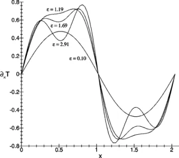
temperature in the fluid layer as shown in Fig. 2. The defor-mation of the rolls due to the presence of secondary harmon-ics is clearly seen in the picture. In order to interpret the results of our measurements for the horizontal temperature gradients, we also plot in Fig. 3 the reconstructed horizontal temperature gradient xT at z⫽0.45 for ⑀⫽0.1, 1.19, 1.69, and 2.91 共again obtained using the four amplitudes model兲. Close to the threshold, the curve is almost a sine function while it becomes more and more deformed as ⑀ is further increased. The deformations are due to the increasing impor-tance of the second and third harmonics of the mode k⫽kc. In particular, for the horizontal temperature gradient, the third harmonics appears clearly for⑀close to 1.19. It is also interesting to note that due to the symmetry of the physical system with respect to z⫽0.5 the second harmonics disap-pears at midheight, as one can see in Fig. 4 where the local extrema due to the third harmonics have all the same abscissa.
IV. GENERALIZED AMPLITUDES METHOD AND COMPARISON WITH NUMERICAL CALCULATIONS The results given in the previous section are in good qualitative agreement with experiments and numerical simu-lations. However, it is possible to improve further, i.e., also get a quantitative agreement. In this section, we build a pre-cise strategy to select the relevant modes that enter the am-plitude equations.
The method developed in Sec. II and leading to Eq. 共16兲 is valid only when the quadratically generated secondary modes have small amplitudes. When⑀is increased, this con-dition is not satisfied and the model is no longer accurate.
Let us first consider a unique amplitude equation for the linearly unstable mode. For the largest value of ⑀ that we have to deal with in the problem 共this value is around three in our case兲, we solve the amplitude equation and determine the value of the amplitude of the basic mode. Then, we
cal-FIG. 2. Stream function共thick lines兲 and temperature field 共thin lines兲 in a plane perpendicular to the rolls for⑀⫽2.91.
FIG. 3. Dimensionless horizontal temperature gradientxT
culate the values of the secondary amplitudes using Eq.共15兲 and check the consistency of the results with the fact that the amplitudes of the secondary modes must remain small with respect to the amplitudes of the basic ones. If a secondary amplitude is larger than some small fraction (10⫺2 in our calculations兲 of the largest amplitude of the basic modes, then we have to include this mode in the basic modes in the next model. This procedure is in fact equivalent to consider-ing terms of order higher than three in Eq. 共16兲 but is much easier. After determining the basic modes of the model, the secondary modes are determined as before: their horizontal wave numbers are equal to the sum or the difference of any two wave numbers of the basic modes. Moreover, for each value of k, it is sufficient to fix Nsl(k)⫽4 or 5 to have convergence of the cubic coefficients of the amplitude equa-tions. This iterative improvement of the model is repeated until all secondary modes have small amplitudes. In the RB problem studied in this paper, this iterative scheme results in a ‘‘generalized’’ 11 amplitude equation model, with, respec-tively, 3, 3, 2, 2, and 1 equations for the amplitudes of the most unstable modes with k⫽0, 1, 2, 3, and 4⫻kc.
The comparison of our theoretical approach and numeri-cal numeri-calculations is presented in Fig. 4 where the horizontal temperature gradient is given as a function of x for z⫽0.5 and for different values of ⑀ (⑀⫽0.1, 1.19, and 2.91). The solid curves correspond to the 11 amplitude equation model while the results for four equations are represented with dot-ted lines. When ⑀ is not too large, the two curves coincide almost perfectly as expected. Far from threshold, the differ-ence becomes significant. We have performed a direct nu-merical simulation of Eqs. 共1兲–共3兲 using theAQUILONcode 共finite volumes PDE solver developed at the MASTER-ENSCPB, Bordeaux, France兲 for ⫽2.91 and the results are
represented by the dots in Fig. 4. The agreement between the direct numerical simulations and the 11 amplitude equation model is excellent and provides a confirmation of the validity of the generalized amplitude equations far from threshold. The iterative procedure is very appealing because it gives a much better understanding of which are the physical relevant convective modes.
V. COMPARISON WITH EXPERIMENTS
We have carried out different experiments to validate the extended amplitude equation model. For each given experi-mental situation, the value of⑀has been determined in terms of the thermophysical parameters and the applied tempera-ture difference between the top and bottom glass plates. The temperature difference across the fluid layer is measured by thermocouples located at the top and bottom surfaces of the fluid. Since the estimated Biot number is very large (Bi ⫽46), the top and bottom plates are almost perfect heat con-ductors and the conductive temperature differenced is
al-most equal to the experimental temperature difference. Therefore, the experimental Rayleigh number 共4兲 is evalu-ated directly in terms of the temperature measurement. The coefficient of thermal expansion of the Rhodorsil 47V100 silicone oil used in experiments is ␣⫽9.54⫻10⫺4 K⫺1. The thermal conductivity was given above (⫽0.16 Wm⫺1K⫺1) and the specific heat at constant pressure is
c⫽1454.4 J K⫺1kg⫺1. Since the experiments are carried out in different temperature ranges, the variations of the density and viscosity with T are taken into account, and we take the value corresponding to the mean temperature of the experi-ment. The phenomenological laws for these variations are given by ⫽988(1⫺␣T) and ln关ln(106)兴⫽⫺1.927 ⫻10⫺3T⫹0.34921, where is the kinematic viscosity and where T in the last expressions is the temperature in Celsius 共it gives Pr⬇880). Using the thermophysical properties and the measured temperature difference, we determine the ex-perimental Rayleigh number. The relative distance to the threshold⑀⫽(Ra⫺Rac)/Racis calculated by using the criti-cal Rayleigh number 1653 previously determined in Sec. II. Data from four different experiments were collected in which the temperature at the bottom of the fluid was fixed to 20, 10, 20, and 40 °C and the temperature differences were 2.41, 5.7, 5.7, and 5.7 °C, respectively. The corresponding values of the relative distance to the threshold are ⑀⫽0.10, 1.19, 1.69, and 2.91, respectively. In all experiments, ten rolls par-allel to the shorter sides were observed. It is well known that the wavelength increases in the nonlinear regime but in the confined problem we consider, with rather small aspect ratios and for rather small values of⑀, the number of rolls is mainly determined by the geometry 关8,18兴. The measured wave number of the eight inner rolls was 2.67 共in dimensionless units兲 and the coefficients of the amplitude equations were recalculated using this experimental value. The comparison between the experimental data for the different values of ⑀ given above and the theoretical predictions is presented in Figs. 5 and 6, where all quantities are expressed in 共dimen-sional兲 SI units. In Fig. 5, the horizontal temperature gradient is represented at midheight of the layer as a function of the
FIG. 4. Dimensionless horizontal temperature gradientxT
ver-sus x at z⫽0.5 and for⑀⫽0.1, 1.19, and 2.91. The dotted and solid lines have been calculated by using 4 and 11 amplitude equations, respectively. The dots correspond to direct numerical calculations
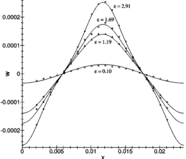
horizontal coordinate. The vertical velocity is displayed in Fig. 6. The solid lines correspond to the predictions of our 11 amplitude equation model while the different symbols repre-sent the experimental data. The agreement between our model and the experiments is very good. Besides experimen-tal error bars, the small discrepancies may be attributed to the fact that the experimental rolls are not perfectly two-dimensional while our theory does not account for three-dimensional effects and for spatial variations of the thermo-physical constants 共computed here at the average temperature兲. It is interesting to note that the agreement is excellent for the velocity because the corresponding mea-surements were carried out in the middle of the box, where the convection is almost 2D. On the contrary, the experimen-tal determination of the temperature gradients is based on an integral method along the rolls 关12兴, for which the 3D as-pects of the motion at both sides of the rolls have some importance.
VI. CONCLUSION
We have shown how the amplitude method, whose valid-ity is theoretically limited to the rather close neighborhood of the convective threshold, may be extended for larger values of ⑀. An a posteriori test of the validity of the results has
been provided, which consists of controlling the smallness of the amplitudes of the secondary modes. If these amplitudes are not small, the corresponding modes must be included in the basic modes and an additional amplitude equation must be considered. This procedure was used to analyze Rayleigh-Be´nard convective rolls and the results were compared to direct numerical calculations as well as to experiments. In both cases, the agreement is excellent. Besides the general-ized amplitude equation technique, our work provides an analysis of the appearance of spatial harmonics of the basic sine pattern in a convective flow and the actual interactions between the different modes are clearly emphasized.
ACKNOWLEDGMENTS
This paper presents results of the Belgian Program Inter-University Pole of Attraction 共IUPA 5兲 initiated by the Bel-gian State, Prime Minister’s Office, Federal Office for Sci-entific, Technical and Cultural Affairs. Support from ESA through the CIMEX-MAP project 共Contract No. 14293/00/ NL/SH兲 and from the European Union through the ICOPAC project 共Contract No. HRPN-CT-2000-00136兲 are cordially acknowledged. It is also a pleasure to thank Professor G. Lebon for stimulating discussions as well as Professor E. Arquis and Professor J. P. Caltagirone 共MASTER Labora-tory, ENSCPB, Bordeaux兲 for providing theAQUILONcode used in our numerical simulations.
关1兴 E.L. Koschmieder, Be´nard Cells and Taylor Vortices 共Cam-bridge University Press, Cam共Cam-bridge, England, 1993兲. 关2兴 P. Colinet, J. C. Legros, and M.G. Velarde, Nonlinear
Dynam-ics of Surface Tension Driven Instabilities共Wiley-VCH, New York, 2001兲.
关3兴 P. Parmentier, V.C. Regnier, G. Lebon, and J.C. Legros, Phys. Rev. E 54, 411共1996兲.
关4兴 V.C. Regnier, P.C. Dauby, P. Parmentier, and G. Lebon, Phys. Rev. E 55, 6860共1997兲.
关5兴 V.C. Regnier, P.C. Dauby, and G. Lebon, Phys. Fluids 12, 2787 FIG. 5. Dimensional 共SI units兲 horizontal temperature gradient
xT versus x at midheight and for⑀⫽0.1, 1.19, 1.69, and 2.91. The
solid curves correspond to the results of the 11 amplitude model with k⫽2.67, while the differents symbols represent the experimen-tal data共see text for details about the experimental conditions兲.
FIG. 6. Dimensional 共SI units兲 vertical velocity w versus x at midheight and for⑀⫽0.1, 1.19, and 2.91. The solid curves corre-spond to the results of the 11 amplitude model with k⫽2.67, while the different symbols represent the experimental data.
共2000兲.
关6兴 P.C. Dauby, P. Colinet, and D. Johnson, Phys. Rev. E 61, 2663 共2000兲.
关7兴 J.K. Platten and J. C. Legros, Convection in Liquids 共Springer-Verlag, Berlin, 1984兲.
关8兴 M. Dubois and P. Berge´, J. Fluid Mech. 85, 641 共1978兲. 关9兴 W.V.R. Malkus and G. Veronis, J. Fluid Mech. 4, 225 共1958兲. 关10兴 A. Schlu¨ter, D. Lortz, and Busse, F., J. Fluid Mech. 23, 129
共1965兲.
关11兴 J.C. Legros and J.K. Platten, Phys. Lett. A 65A, 89 共1978兲. 关12兴 P. Cerisier, J. D. Sylvain, and P.C. Dauby, Exp. Fluids 共to be
published兲.
关13兴 P. Cerisier, S. Rahal, J. Cordonnier, and G. Lebon, Int. J. Heat Mass Transf. 41, 3309共1998兲.
关14兴 C. Canuto, M.Y. Hussaini, A. Quarteroni, and T.A. Zhang, Spectral Methods in Fluid Mechanics共Springer-Verlag, Berlin 1988兲.
关15兴 P.C. Dauby and G. Lebon, J. Fluid Mech. 329, 25 共1996兲. 关16兴 P. Manneville, Dissipative Structures and Weak Turbulence
共Academic Press, New York, 1990兲.
关17兴 H. Haken, Advanced Synergetics 共Springer-Verlag, Berlin, 1983兲.