Étude en laboratoire de l’injection de mousse pour le traitement de sols contaminés aux hydrocarbures.

Université du Québec

Institut national de la recherche scientifique Centre Eau Terre Environnement

ÉTUDE EN LABORATOIRE DE L’INJECTION DE MOUSSE POUR LE

TRAITEMENT DE SOLS CONTAMINÉS AUX HYDROCARBURES

Par

Mélanie Longpré-Girard

Mémoire présenté pour l’obtention du grade de Maître ès sciences (M.Sc.)

en Sciences de la Terre

Jury d’évaluation

Président du jury et Guy Mercier

examinateur interne INRS ETE

Examinateur externe Daniel Cassidy

REMERCIEMENTS

Je tiens tout particulièrement à remercier Thomas Robert pour l’aide et les encouragements qu’il m’a patiemment prodigués durant chacune des étapes de ce projet. Je tiens également à remercier mes directeur et codirecteur Richard Martel et René Lefebvre pour tout le support qu’ils m’ont apporté. Je tiens particulièrement à les remercier pour la liberté qu’ils m’ont accordée autant dans l’élaboration que dans l’exécution de ce projet. Je veux remercier Jean-Marc Lauzon et TechnoRem pour leur intérêt dans le projet. Je me dois aussi de remercier tous les gens merveilleux de l’équipe de l’INRS qui m’ont aidé pendant le projet : Luc Trépanier, Uta Gabriel et Richard Lévesque.

Et je remercie spécialement mes amis et ma famille qui m’ont soutenu tout au long de ce projet. Enfin, je tiens à remercier Guillaume Lefrançois, qui m’a supportée avec affection tout au long de ce projet.

RÉSUMÉ

L’injection de mousse pour la réhabilitation de sols contaminés aux hydrocarbures légers est une méthode prometteuse. Ce projet porte sur le développement d’une méthodologie de production de mousse et sur l’étude du comportement rhéologique de cette mousse lorsqu’elle est injectée dans un milieu poreux hétérogène. Plusieurs solutions tensioactives ont été testées afin d’identifier le meilleur candidat pour le traitement de sable de silice hétérogène contaminé au p-xylène. Les tensioactifs ont été départagés suivant leur capacité à produire de la mousse via des mesures Ross Miles et leur habilité à abaisser la tension interfaciale de la solution avec le p-xylène grâce à la méthode de la goutte pendante. Pour les tensioactifs sélectionnés, il a été constaté que le test Ross Miles fournit une comparaison adéquate des propriétés moussantes des solutions puisque les candidats ayant eu les meilleurs résultats Ross Miles ont par la suite produit les mousses les plus visqueuses en colonne. D’autres essais en colonne ont indiqué que pour obtenir le front de mousse le plus stable et visqueux possible, il faut utiliser une colonne de production de mousse, pré-rincer la colonne avec la solution tensioactive avant l’injection de la mousse et utiliser une pression d’injection élevée.

Un bac 2D contenant deux couches de sables de granulométries différentes a été utilisé pour évaluer le contrôle de mobilité obtenu lors de l’injection la mousse. Le contraste de perméabilité entre les deux couches a été constaté lors de l’essai de traçage où des fronts de traceur en forme de piston ayant des vitesses différentes dans chaque couche ont été observés. L’essai d’injection de mousse dans le bac non contaminé a permis l’observation d’un front en forme de « S » avançant à la même vitesse dans chaque couche ce qui indique un meilleur contrôle de mobilité que lors de l’essai de traçage. Suite à la contamination du bac au p-xylène, un essai de traçage a permis de constater l’augmentation du contraste de perméabilité entre les deux couches de sable. Un premier traitement avec une solution tensioacive a eu pour effet de remobiliser une partie du p-xylène sans en récupérer à la sortie du bac. L’injection de mousse a permis d’atteindre une saturation résiduelle sous la limite de détection de 16 mg/kg dans les zones balayées par la mousse ce qui est sous le critère (50 mg/kg) acceptable pour un terrain à

TABLE DES MATIÈRES

CHAPITRE 1 : INTRODUCTION ... 1

1.1 CADRE DU PROJET ... 1

1.1.1 Restauration in situ à l’aide de solutions tensioactives ... 1

1.1.2 Restauration in situ à l’aide des mousses ... 2

1.2 OBJECTIFS DE RECHERCHE ... 2

1.3 ORGANISATION DU MEMOIRE ... 3

CHAPITRE 2 : THEORIE ... 5

2.1 INTRODUCTION ... 5

2.2 PROPRIETES DES TENSIOACTIFS ... 6

2.3 PROPRIETES DES MOUSSES ... 7

2.4 FORCES EN PRESENCE ... 8

CHAPITRE 3 : SURFACTANT FOAM SELECTION FOR ENHANCED LNAPL RECOVERY IN CONTAMINATED AQUIFERS ... 11

RESUME ... 11

ABSTRACT ... 12

3.1 INTRODUCTION ... 12

3.1.1 Enhanced NAPL recovery mechanisms with surfactants and foams ... 13

3.1.2 Foam properties ... 14

3.1.3 Research objectives ... 15

3.2 METHODOLOGY ... 16

3.2.1 Surfactant selection methodology ... 16

Foamability ... 18

Interfacial tension ... 19

3.2.2 Foam production and injection system ... 20

3.2.3 Sand column experiments ... 21

viii

Effect of water or surfactant pre-flush ... 28

Effect of surfactant type ... 30

Effect of injection pressure ... 32

3.4 DISCUSSION ... 34

3.5 CONCLUSIONS ... 36

3.6 ACKNOWLEDGEMENTS ... 37

CHAPITRE 4 : 2D SANDBOX EVALUATION OF FOAMS FOR MOBILITY CONTROL AND ENHANCED LNAPL RECOVERY IN LAYERED SOILS ... 39

RESUME ... 39

ABSTRACT ... 40

4.1 INTRODUCTION ... 41

4.1.1 Overview ... 41

4.2 THEORY ... 42

4.2.1 NAPL enhanced recovery mechanisms with surfactants and foams ... 42

4.2.2 Mobility control with polymers and foams ... 43

4.3 METHODOLOGY ... 44

4.3.1 2D Sandbox experimental setup ... 44

4.3.2 Water and p-xylene saturation ... 47

4.3.3 Tracer tests ... 49

4.3.4 Foam injection ... 50

4.3.5 Sampling and analytical methods... 51

4.4 RESULTS AND DISCUSSION ... 51

4.4.1 Overall Conductivity and Porosity ... 51

4.4.2 Tracer tests ... 52

4.4.3 Uncontaminated foam test ... 55

4.4.4 LNAPL remediation ... 57

4.5 CONCLUSIONS ... 63

4.6 ACKNOWLEDGEMENTS ... 64

CHAPITRE 5 : CONCLUSIONS GENERALES ET RECOMMANDATIONS ... 65

LISTE DES TABLEAUX

Tableau 2.1 – Propriétés physicochimiques du p-xylène et de l’essence. ... 5 Table 3.1 – List of tested surfactants. ... 17 Table 3.2 – Properties of Temisca 20 sand used in column experiments. d10 and d50 refer to grain

sizes larger than 10% and 50%, respectively, of sand mass. ... 21 Table 3.3 – Summary of column tests including the characteristics of each test, a concentration of

0.1% w/w was used for all tests. ... 26 Table 3.4 – Summary of the parameters evaluated with the corresponding column tests and figures. ... 26 Table 3.5 – Summary of column test results and conclusions. ... 34 Table 4.1 – Properties of silica sands used for sandbox tests, d10 and d50 refer to grain sizes larger

than 10% and 50%, respectively, of sand mass. ... 46 Table 4.2 – Total pore volume in the sandbox based on measurements made during sandbox filling

and by weighting the sandbox dry and saturated (ml) ... 52 Table 4.3 – Effective permeability contrasts. ... 55 Table 4.4 – Foam injection removal for each remediation mechanism and hypothesized recovery with

LISTE DES FIGURES

Figure 2.1 – Structure des parois des bulles de mousse, l’air est en jaune, la solution tensioactive en bleu et le LI en rouge. (modifié à partir de Farajzadeh et al., 2012) ... 7 Figure 3.1 - Apparatus used for the Ross Miles Test ... 18 Figure 3.2 - Experimental setup for foam production and injection into sand columns. T-1 through T-4

refer to pressure transducers. Films were made of foam flow through the acrylic sand column. ... 21 Figure 3.3 –Foamability of surfactant solution at concentrations of 0.01%, 0.1% and 1% measured

with the Ross Miles Test for all tested surfactants (A through M; see Table 4.1). ... 24 Figure 3.4 - Interfacial tension between p-xylene and the tested surfactant solutions at concentrations

of 0.01%, 0.1% and 1% (A through M; see Table 3.1). ... 24 Figure 3.5 - Foamability expressed as foam height (cm) of selected surfactant solutions measured

with the Ross Miles Test at three different times at 0.1% concentration. ... 25 Figure 3.6 - Interfacial tension (mN/m) between p-xylene and the selected three different surfactant

solutions at 0.01%, 0.1% and 1% concentrations ... 25 Figure 3.7 - Advancing foam front of surfactant A (0.1% w/w concentration) injected downward

following a surfactant pre-flush at a constant pressure of 350 cm water in a Temisca 20 sand column with and without a foam production column. The black dotted line indicates the foam front position. ... 27 Figure 3.8 – Calculated foam viscosity (mPa∙s) of foam produced with 0.1% concentration surfactant

A solution in sand column with and without a foam production column using the Front Velocity and Output methods ... 28 Figure 3.9 - Advancing foam front of surfactant B injected downward at a pressure of 350 cm H2O in

the sand column pre-flushed with water or liquid surfactant as a function of time (minutes). The black dotted line indicates the foam front position. ... 29 Figure 3.10 – Calculated 0.1% concentration surfactant B solution foam viscosity in sand column

when pre-flushed with water or liquid surfactant using the Front Velocity and Output methods ... 29 Figure 3.11– Foam front velocity of surfactant B solution 0.1% foam injected in Temisca 20 sand

column pre-flushed with water or surfactant solution B 0.1%. The black dotted line indicates the foam front position. ... 30 Figure 3.12 - Advancing foam front of surfactants A, B and I (at a concentration of 0.1%) injected with

a foam production column downward at a pressure of 350 cm H2O in a sand column pre-flushed with their respective surfactant solution. The black dotted line indicates the foam front position. ... 31 Figure 3.13 - Calculated foam viscosity in Temisca 20 sand column injected with surfactants A, B and

xii

Figure 4.2 – (a) Schematized nylon distribution chamber details; distribution chamber closed by a perforated plate overlaid by a stainless steel mesh screen. (b) Schematized empty sandbox with distribution chambers shown. T-1 through T-4 refer to pressure transducers. ... 45 Figure 4.3 – Photo of the distribution of contaminant in sandbox after the first saturation with p-xylene... 47 Figure 4.4 – Photos of contaminant saturation of Flint layer in sandbox through time achieved by

pumping in pressure ports while sandbox is upside down (a) initially, and after (b) 3h30, (c) 5h30 and (d) 15h00 ... 48 Figure 4.5 – Photos of p-xylene saturated sandbox placed on its short side and rinsed from bottom to

top with water to bring it to residual saturation, after (a) 9 ml, (b) 20 ml, (c) 70 ml, (d) 150 ml and (e) 14 L of water injection. ... 49 Figure 4.6 – Photos of tracer test in the uncontaminated sandbox, white lines indicate the position of

the tracer front after (a) 0.5 PV, (b) 1 PV, (c) 1.5 PV, (d) 2 PV and (e) 2.75 PV (PV is based on the total pore volume in the entire sandbox). ... 53 Figure 4.7 – Photos of the tracer test carried out in the contaminated sandbox, the white lines indicate

the position of the tracer front after (a) 0.5 PV, (b) 1 PV, (c) 1.5 PV, (d) 2 PV and (e) 2.9 PV (1PV is 453 ml). ... 54 Figure 4.8 – Uncontaminated and contaminated sandbox bromide tracer arrival curves. ... 55 Figure 4.9 – Photos of foam injection experiment in uncontaminated sandbox after (a) 1 min, (b) 5

min, (c) 29 min, (d) 59 min and (e) 2 hours 5 min. ... 56 Figure 4.10 - Photos of contaminated sandbox pre-flushed with liquid surfactant prior to foam

treatment, (a) initially and after (b) 0.55 PV, (c) 1.1 PV and (d) 2.2 PV. (1 PV is 453 ml) ... 57 Figure 4.11 – Photos of foam treatment of contaminated sandbox (a) 34 min (b) 2h 30 min (c) 12 h (d)

26 h (e) 46 h ... 58 Figure 4.12 – P-xylene recovery with each mechanism and combined. PV is 548 ml. ... 60 Figure 4.13 – Photos of foam injection in the contaminated sandbox after an overnight stop. The black

line is the position of the front before the overnight pause, the yellow line is the foam front actual position. Photos show (a) initial conditions after the overnight stop and (b) 1 min, (c) 5 min, (d) 15 min and (e) 55 min after foam injection had resumed. ... 61 Figure 4.14 – Photos of foam injection in inverted configuration sandbox (coarser layer under finer

layer), the black line indicates the foam front locations after (a) 7 sec, (b) 46 sec, (c) 4 min and (d) 1 hour after the start of injection in a non-contaminated sandbox. ... 63

CHAPITRE 1

: INTRODUCTION

1.1 Cadre du projet

Cette étude a été réalisée dans l’optique d’une application de mousses produites avec des tensioactifs en solutions aqueuses sur des sites contaminés aux liquides immiscibles légers (LIL). Ce projet est financé par une subvention de recherche et développement coopérative du Conseil de Recherches en sciences naturelles et en génie du Canada (CRSNG-RDC) en partenariat avec TechnoRem, Laval, Canada. Il vise à étudier le comportement des mousses en laboratoire dans l’optique d’une application à l’échelle terrain pour réhabiliter des sites contaminés aux LIL.

1.1.1 Restauration in situ à l’aide de solutions tensioactives

L’utilisation des solutions tensioactives pour récupérer des hydrocarbures dans les sols a été extensivement étudiée par le passé. L’industrie pétrolière est responsable d’une majeure partie des recherches sur les tensioactifs menées en récupération assistée du pétrole (RAP) dans les réservoirs pétroliers profonds (Lake, 1989). Cependant, les conditions sont différentes entre les réservoirs pétroliers profonds et les sédiments contaminés peu profonds. Les réservoirs pétroliers sont souvent situés à des profondeurs où la température et les pressions d’injection des fluides sont élevées sans craintes d’instabilités ou de fracturation du réservoir. Dans les sédiments peu profonds, les températures sont basses et les fluides doivent être injectés à une pression qui n’excède pas la masse de sol saturée au-dessus de la zone traitée pour ne pas engendrer d’instabilités et un soulèvement des sols (Chowdiah et al.,1998). De plus, les solutions utilisées en traitement de sédiments doivent être biodégradables et non toxiques puisqu’une migration post-traitement est possible. En RAP, les profondeurs auxquelles les fluides sont injectés étant grandes, la migration des produits vers des récepteurs potentiels est improbable et la toxicité des tensioactifs n’est pas aussi critique qu’en environnement.

2

combinés avec la solution tensioactive. Ces fluides stabilisent le front d'injection et assurent le passage du fluide injecté non seulement dans les couches très perméables mais aussi dans les couches de faible perméabilité qui ne seraient normalement pas contactées par les tensioactifs. Cette option a été étudiée dans le cadre de nombreuses recherches (Martel, 1995; Martel et al.,1998; Martel et al., 2004; Silva et al., 2012; Robert et al., 2006). Les polymères agissent de deux façons : ils augmentent la viscosité de la solution ce qui assure la stabilité du front du fluide injecté, et leur propriété rhéofluidifiantes entraînent une diminution de la viscosité lorsque la force de cisaillement est élevée comme c’est le cas près des puits d'injection et lors du passage dans des horizons de sédiments fins.

1.1.2

Restauration in situ à l’aide des mousses

Tout comme certains polymères, la mousse possède des propriétés nonnewtoniennes et rhéofluidifiantes (Hirasaki et Lawson, 1985; Falls et al., 1989). De plus, la présence d’air entraîne une diminution de la perméabilité relative du milieu à l’eau ce qui permet un meilleur contrôle de mobilité (Li, 2011). Le grès fracturé est souvent considéré comme un milieu poreux favorable à l’injection de mousse en RAP (Simjoo et al., 2012; Nguyen et al.. 2007). Plusieurs études ont été menées sur les mousses pour la réhabilitation de sites contaminés par des liquides immiscible denses (LID) tels que le TCE (Jeong and Corapcioglu, 2000, 2003, 2005; Rothmel et al., 1998; Pennell et al., 1996). Cependant, pour ce type de contamination, la mobilisation du contaminant n’est pas désirée puisque le contaminant plus dense que l’eau peut être entraîné en profondeur ce qui le rend plus difficile à récupérer. Dans le cas d’un LIL, la migration verticale ne pose pas problème étant donné qu’il a tendance à migrer vers le haut de la zone saturée, ce qui le rend plus facile à récupérer. Cette étude a été réalisée dans l’optique de traiter un LIL avec des mousses capables de mobiliser la contamination trappée dans un milieu poreux hétérogène peu profond.

1.2 Objectifs de recherche

L’objectif principal de cette étude est de développer une méthodologie pour la sélection d’un tensioactif et pour la production de mousse dans le but de traiter une contamination au LIL dans des sédiments peu profonds. Pour atteindre cet objectif, les objectifs secondaires suivants ont été fixés :

- Sélectionner un tensioactif capable de produire une mousse propice à la récupération de LIL trappé dans des sédiments peu profonds. Cette sélection est basée sur la caractérisation des propriétés de la mousse (qualité de la mousse, viscosité de la mousse et capacité à mousser) ainsi que sur le pouvoir mobilisant du tensioactif;

- Produire de la mousse ex situ et l’injecter dans un milieu poreux homogène afin de la caractériser sous des conditions représentatives de sédiments peu profonds ainsi que de vérifier l’effet sur le comportement de la mousse de deux conditions: la pression d’injection, le prélavage du milieu poreux avec de l’eau ou le tensioactif en solution utilisé pour produire la mousse;

- Dans un bac de sable 2D, évaluer l’effet de l’hétérogénéité sur le comportement de la mousse ainsi que la récupération de LIL grâce à son injection dans un milieu poreux constitué de deux couches de sables superposées de perméabilités différentes.

Plusieurs types de tensioactifs ont été évalués pour leur capacité à produire de la mousse et à mobiliser le contaminant. Les propriétés d’écoulement de la mousse en milieu poreux 1D sont évaluées grâce à des colonnes d’acrylique transparentes simulant un milieu poreux homogène. Les propriétés de la mousse sont observées dans ces colonnes par suivi visuel et des pressions dans le système. L’étude de l’écoulement de la mousse en milieu hétérogène est possible grâce à la conception et la production d’un bac 2D permettant de reproduire en laboratoire un milieu poreux stratifié constitué de deux couches de sable de perméabilités différentes. Des essais d’injection de traceur et de mousse ont été effectués dans le bac avant sa contamination. Des essais de traçage, de traitement avec une solution tensioactive et de traitement avec de la mousse ont été effectués dans le bac contaminé.

1.3 Organisation du mémoire

4

fournir des indications pour les essais en bac 2D présentés au Chapitre 4. Ce dernier prend aussi la forme d’un article et porte sur les essais en bac de sable; la méthodologie utilisée ainsi que les résultats des différents essais effectués. Le chapitre 5 fait état des principales conclusions tirées au cours du projet

Les chapitres 3 et 4 présentent le corps du projet, plusieurs auteurs ont donc participé à leur réalisation. L’auteure du présent mémoire a effectué la planification ainsi que l’exécution des essais de laboratoire. Elle a aussi effectué la rédaction des deux articles présentés. Thomas Robert a participé à l’exécution de certains essais de laboratoire ainsi qu’à la planification de la méthodologie utilisée dans le cadre du projet. Richard Martel, René Lefebvre et Jean-Marc Lauzon ont effectué la planification du projet. Richard Martel et René Lefebvre ont effectué la révision des articles ainsi que la validation de la méthodologie utilisée. Jean-Marc Lauzon a participé au financement du projet par l’entremise de TechnoRem.

CHAPITRE 2

: THÉORIE

2.1 Introduction

Au Québec, en 2010, 65% de sites contaminés recensés par l’actuel Ministère du Développement durable de l’Environnement et de la Lutte contre les changements climatiques (MDDELCC) contenaient des hydrocarbures C10-C50 (Hébert et Bernard, 2013). Une des catégories importantes composant ce groupe de contaminants est les BTEX (benzène, toluène, éthylbenzène et xylène) qui sont les produits principalement trouvés dans l’eau souterraine suite à une contamination à l’essence. Donc, afin de représenter l’essence altérée par un passage dans le sol, le p-xylène, un des BTEX, a été choisi puisque ses propriétés physicochimiques (Tableau 2.1) sont conservatrices par rapport à celles de l’essence dans un contexte de réhabilitation. La densité et la viscosité du p-xylène étant plus élevées que celles de l’essence, il est donc moins mobile dans un milieu poreux. Sa pression de vapeur étant plus faible que celle de l’essence même lorsqu’altérée, le p-xylène est donc moins volatile. Le choix du p-xylène permet l’utilisation d’un produit pur de grade laboratoire moins volatile et moins toxique que l’essence.

Tableau 2.1 – Propriétés physicochimiques du p-xylène et de l’essence.

Produit Chimique Densité (kg/m³) Viscosité (mPa∙s) Pression de vapeur (atm) à 20°C p-xylène 0.86111 _0.6441 _0.0086² Essence 0.73211 _0.451 _0.34² Essence altérée* - - 0.049²

* Telle que définie par Johnson et al. (1990) 1 Mercer et Cohen (1990)

² Johnson et al. (1990)

CH H C

6

2.2 Propriétés des tensioactifs

Les tensioactifs (surfactants en anglais) sont communément appelés détergeants, il s’agit de produits purs ou de mélanges constitués de molécules ayant une tête hydrophile et une queue hydrophobe. Les molécules, lorsque seules, sont appelées monomères. Lorsque la concentration en tensioactif dans l’eau dépasse une certaine valeur appelée concentration micellaire critique (CMC), les monomères peuvent s’agréger en structures appelées micelles. Ces structures sont constituées de plusieurs monomères dont la tête hydrophile est dans l’eau et la queue hydrophobe est orientée vers l’intérieur de la micelle. Il existe toutes sortes de formes de micelles (sphérique, bâtonnets, etc.) et les micelles d’un même tensioactif peuvent varier de forme suivant la concentration.

Les tensioactifs se divisent en plusieurs types suivant la charge ionique de leur tête hydrophile. Les tensioactifs anioniques ont une charge négative, les cationiques positive et les anioniques n’ont pas de charge. Il existe aussi un type de tensioactifs appelé amphotère, ceux-ci peuvent avoir une charge positive ou négative dépendamment du pH. Ces différents types ont des propriétés différentes particulièrement en ce qui a trait à l’adsorption sur les particules de sol. Lorsqu’il y a présence d’une interface entre le tensioactif dans l’eau et un fluide immiscible, l’air par exemple, les monomères vont partitionner à l’interface en s’orientant de façon à ce que leur tête hydrophile soit dans l’eau et leur queue hydrophobe soit dans l’air. Ils vont ainsi modifier un paramètre appelé la tension interfaciale (σ) ou, lorsque le fluide en contact avec le tensioactif est de l’air, appelé tension de surface. La tension interfaciale est définie comme l’énergie nécessaire pour créer une nouvelle unité de surface à l’interface entre deux fluides non immiscibles. Elle est donc définie par un travail par unité de surface :

𝜎 =𝑇𝑟𝑎𝑣𝑎𝑖𝑙 𝐴𝑖𝑟𝑒 = 𝐹𝑑𝑥 𝑑𝐴 [=] [ 𝑘𝑔 𝑠²] [=] [ 𝑁 𝑚] Équation 2.1

Donc, plus la tension interfaciale est petite, plus la force nécessaire pour créer une unité de surface est petite et plus les deux fluides immiscibles sont facilement liables.

La mouillabilité d’un fluide se définit comme la capacité de ce fluide, lorsque présent avec un autre fluide, à adhérer ou à s’étaler sur une surface solide. La mouillabilité s’exprime par l’angle de contact (Ө) d’une goutte en contact avec une surface solide, l’angle de contact mesuré est celui dans la phase aqueuse. Par exemple, dans un système composé d’eau (w), d’huile (o) et d’une surface solide (s), la mouillabilité à l’huile exprime la tendance relative de l’huile à

s’étendre sur la surface solide lorsque baignant dans l’eau. Dans le cas d’un sable de silice, le milieu est hydrophile et donc la mouillabilité est à l’eau ce qui implique que le LI occupe le milieu des grands pores.

2.3 Propriétés des mousses

La mousse est un ensemble composé d’un mélange d’air et de liquide. La phase liquide est continue et au moins une partie de la phase gazeuse est discontinue par la présence de minces films de liquides. Donc, lorsque la partie liquide de la mousse est constituée par une solution tensioactive, les parois des bulles sont constituées d’une double couche de monomères ayant la tête hydrophile dans le liquide et la queue hydrophobe dans l’air. De même, lorsqu’il y a présence de liquide immiscible, l’organisation des monomères demeure la même excepté le fait que les monomères situés sur une des doubles couches ont la queue hydrophobe dans le LI tel qu’illustré à la Figure 2.2. La baisse de tension interfaciale entre la solution tensioactive et le LI peut aussi entraîner la formation de fines bulles de LI qui se logent dans les parois des bulles de mousse, permettant ainsi la mobilisation du LI.

Film mouillant Solution tensioactive Film symétrique (gaz/eau/gaz) Film asymétrique (LI/eau/gaz) Gaz Solide LI Tensioactif

8

tensioactive et de l’air (Hirasaki et Lawson, 1985; Manlowe et Radke, 1990). Cette augmentation en terme de viscosité est due à deux phénomènes (Falls et al., 1989) : le cisaillement des parois des bulles entre les parois des pores et l’interface avec l’air et la force nécessaire à appliquer sur les parois des bulles afin de permettre leur passage dans les pores de taille restreinte.

2.4 Forces en présence

Afin de créer un système efficace pour récupérer un LI, il faut d’abord comprendre les forces en présence qui trappent le LI dans les pores :

La force gravitationnelle (ΔPg) est une force hydrostatique qui dépend du contraste de densité (Δρ) entre le LI et l’eau, de la hauteur (h) du LI et de la constante gravitationnelle (g). Dans le cas d’un LIL comme le p-xylène, la force gravitationnelle pousse le LI à migrer vers le haut.

∆𝑃_𝑔= ∆𝜌𝑔ℎ Équation 2.2

La force capillaire (Pc) résulte de la différence de pression entre deux fluides immiscibles mesurée à l’interface courbe les séparant. Elle dépend de la tension interfaciale entre l’eau souterraine et le LI (σ), de l’angle de contact entre une gouttelette de LI et le sol (θ) et du rayon (r) du pore dans lequel se trouve la gouttelette. La force capillaire retient le LI dans les pores et restreint sa mobilisation.

𝑃_𝑐 =2𝜎𝑐𝑜𝑠𝜃 𝑟

Équation 2.3

La force visqueuse (Pv) résulte de l’écoulement du fluide déplaçant dans les pores qui pousse le LI dans le milieu poreux. Cette force dépend du flux (q) du fluide déplaçant, de sa viscosité (µ), de la longueur (L) de la gouttelette qui est poussée et de la perméabilité intrinsèque du milieu (k).

𝑃_𝑣=𝑞𝜇𝐿

𝑘 Équation 2.4

La mobilisation d’une gouttelette de LI aura lieu lorsque la force visqueuse dépasse la force capillaire. Le nombre capillaire (Nc) est le rapport entre ces deux forces et donne une indication sur les paramètres pouvant être modifiés afin de mobiliser le LI.

𝑁𝑐 =

𝑞𝜇

𝜎𝑐𝑜𝑠𝜃 Équation 2.5

Pennell et al. (1996) ont évalué qu’un nombre capillaire se situant entre 1x10-5 _{et 5x10}-5 _était nécessaire pour déclencher la mobilisation du TCE dans un sable de silice homogène et qu’un nombre capillaire de 1x10-3 _{était nécessaire pour récupérer entièrement le TCE dans les} mêmes conditions. Dans cette optique, il est nécessaire d’optimiser le nombre capillaire afin d’augmenter la récupération des LIL par mobilisation.

CHAPITRE 3

: SURFACTANT FOAM SELECTION FOR ENHANCED

LNAPL RECOVERY IN CONTAMINATED AQUIFERS

Mélanie Longpré-Girarda_{, Richard Martel}a_{, Thomas Robert}a_{, René Lefebvre}a_{, Jean-Marc} Lauzonb

a _{INRS-Eau, Terre et Environnement, Institut national de la recherche scientifique, Université du Québec, 440}

Boul. de la Couronne, Québec, Québec, Canada, G1K 9A9

b _{TechnoRem Inc., 4701 Rue Louis B Mayer, Laval, Québec, Canada, H7P 6G5}

Résumé

Cette étude avait pour but d’élaborer une méthodologie permettant le choix d’un tensioactif ainsi que des paramètres d’injection pour la production d’une mousse capable de traiter un sol contaminé au p-xylène. Deux critères de sélection ont été considérés pour le choix du tensioactif : la moussabilité grâce au test Ross Miles et la tension interfaciale avec le p-xylène grâce à la méthode de la goutte pendante. Trois tensioactifs ont été identifiés suite à ces tests : (1) Genapol LRO qui a la meilleure moussabilité; (2) Ammonyx Lo qui a la tension interfaciale la plus basse et qui a la seconde meilleure moussabilité et ; (3) Tomadol 900 qui a été choisi à des fins de comparaisons puisqu’il présente des résultats moyens pour les deux tests. La production de mousse de chacun de ces trois tensioactifs a été testée en colonne et les résultats concordaient avec les essais Ross Miles ; Genapol LRO a produit une mousse si visqueuse que le front est devenu instable à la fin de l’essai alors que Ammonyx Lo a produit une mousse moins visqueuse mais stable tout au long de l’essai, Tomadol 900 a produit une mousse peu visqueuse et instable. Les autres tests en colonne ont permis de déterminer les paramètres d’injection de mousse optimaux afin de produire un front de mousse stable et uniforme : une colonne de production de mousse doit être utilisée, un pré-rinçage de la colonne avec le tensioactif doit être fait avant l’injection de mousse et l’injection de mousse doit se faire à haute pression. Cette étude monte que d’autres essais sont requis afin d’évaluer la stabilité du front de mousse lors d’une injection horizontale dans des dépôts hétérogènes stratifiés.

12

Abstract

This study aimed to develop a methodology for surfactant selection for foam production and foam injection conditions for the treatment of a p-xylene contaminated soil. Two critera were determined for surfactant selection: foamability evaluated with the Ross Miles test and interfacial tension reduction measured with the Pendant Drop method. Three surfactants were identified following these tests: Genapol LRO because it is producing the highest foam height in the Ross Miles test, Ammonyx Lo which is having the lowest interfacial tension with p-xylene and the second highest foam height and Tomadol 900 for comparison purposes because it had intermediate results in both tests. Foam production of each surfactant was tested in a sand column and results showed the same ranking in foam viscosities than in foamabilities: Genapol LRO produced a foam so viscous that it was destabilized at the end of the experiment, Ammonyx Lo produced a less viscous foam but with a stable front throughout the experiment and Tomadol 900 produced an unstable foam with poor viscosity. The other column tests gave indications on the optimal conditions needed to produce a stable and viscous foam front: a production column must be used, a pre-flush with surfactant solution (having the same concentration and surfactant used in foam) must be done prior to foam injection and injection pressure must be high. This study showed that other tests are needed in order to evaluate the impact of horizontal foam injection through stratified soil layers on foam front behavior.

3.1 Introduction

Many studies on surfactant foam have been carried out in the petroleum industry for the application of foams to enhanced oil recovery (EOR) in deep oil reservoirs (Li et al. 2012a; Farajzadeh et al., 2012; Shallcross et al., 1990). Also, EOR studies often consider fractured sandstone as a favorable porous media for foam injection (Simjoo et al., 2012; Nguyen et al., 2007). However, environmental applications under field conditions are quite different from EOR. Shallow sites contaminated by organic compounds are mainly in unconsolidated porous materials, a low injection pressure must be used to prevent soil heaving and the natural groundwater present in the pores is not saline. Still, few laboratory studies have been carried out to assess foam behavior in porous media for their application to the remediation of shallow contaminated soils (Mulligan and Eftekhari, 2003; Couto et al., 2009, Tanzil et al. 2002a). The application of foams to the remediation of Light Non-Aqueous Phase Liquids (LNAPL) is studied

here, whereas some of the previous work considered Dense Non-Aqueous Phase Liquids (DNAPL), such as TCE, as the contaminant type to be removed (Jeong and Corapcioglu, 2000, 2003, 2005; Rothmel et al., 1998; Pennell et al., 1996). For a DNAPL, mobilization has to be avoided to prevent the sinking of contaminants, which would worsen site contamination. Some field-scale tests of foam injection in shallow soils were also conducted (Hirasaki et al., 2000). Our study was done in the context of an application of foam to remediate LNAPL-contaminated soils with a specific LNAPL, p-xylene. The objective was to develop a methodology for: (1) the selection of surfactants for foam injection, (2) the ex situ production of foam, and (3) the injection of foam in a sand column in order to observe its behavior in a porous media. This laboratory study was intented to provide a basis to assess the feasibility of such an application of foam for LNAPL-contaminated shallow soils. This paper describes the methodology developed for surfactant selection, foam production and injection, and foam behavior in a 1D sand column.

3.1.1 Enhanced NAPL recovery mechanisms with surfactants and foams

Two recovery mechanisms take place during foam injection for DNAPL remediation: dissolution and volatilization (Mulligan and Eftekhari, 2003). When a LNAPL is treated, however, mobilization can be added to the list and it becomes the main mechanism. To minimize costs, low concentrations of surfactant are used for foam production, which means that enhanced dissolution would be low. LNAPL recovery with volatilization would also be small compared to mobilization because of the limiting factor of transfer from the NAPL phase to the air phase. NAPL may be mobilized due to the increase of the capillary number (Nc), which is defined as follows (Pennell et al., 1996):

𝑁_𝑐 = 𝜇𝑞

𝜎𝑐𝑜𝑠𝜃 Equation 3.1

The increase in viscous forces is achieved by increasing the injected fluid viscosity (

𝜇)

14

mobilization because, compared to water, it increases viscosity and decreases interfacial tension by at least one order of magnitude. Interfacial tensions were therefore measured for several surfactants and the best candidates with the lowest interfacial tension with the contaminant were considered for further investigation.

3.1.2 Foam properties

Foam flow through porous media is defined by Hirasaki (1989) as a “dispersion of gas in liquid such that the liquid phase is continuous (i.e. connected) and at least some part of the gas phase is made discontinuous by thin liquid films called lamellae”. Foam has non-Newtonian and shear-thinning properties (Hirasaki, 1985; Falls, 1989), which makes foam an alternative solution to the use of polymers for mobility control. Also, the presence of air in foam reduces significantly the amount of surfactant needed to sweep a given volume, compared with surfactant solution injection. Thus, when compared with surfactant solutions, the use of foam can lower the volume of surfactant needed and even replace the use of polymers.

Two conditions were considered in this study to characterize foam-forming surfactants: foamability and foam quality. Foam has dynamic nature, its properties evolving significantly through time. Furthermore, the same surfactant can produce foam with different properties depending on the production method. So, to make sure conditions can be compared between different surfactants, the same foam production method and the same measurement conditions need to be used.

Foam quality is used to evaluate the air content of the foam and is defined by the following expression (Chowdiah et al., 1998):

𝐹𝑜𝑎𝑚 𝑄𝑢𝑎𝑙𝑖𝑡𝑦 = 𝐺𝑎𝑠 𝑣𝑜𝑙𝑢𝑚𝑒

𝑇𝑜𝑡𝑎𝑙 𝑣𝑜𝑙𝑢𝑚𝑒 Equation 3.2

For the purposes of this study, foamability is considered as the height of foam produced during a Ross Miles Test, as described by Li et al. (2012b). This test involved the use of a fixed volume of surfactant solution that falls in a receiving tube of a certain height into a constant volume of the same surfactant solution.

Foam viscosity cannot be measured with conventional methods because of its dynamic nature. It is therefore necessary to assess the apparent viscosity (μapp) of foam as it flows in a horizontal

1D porous media using Darcy’s Law in its generalized form for the flow of any Newtonian fluid (Bear, 1972; Marsily 1986):

𝜇_𝑎𝑝𝑝=𝑘∇𝑃

𝑞 Equation 3.3

Where k is the intrinsic permeability (m²), ∇P is the pressure gradient (Pa/m) and q is the volumetric flux (m³/m2_{s or m/s).}

3.1.3 Research objectives

The general objective of this study was to develop a methodology for the selection of a surfactant and foam production in order to remediate LNAPL-contamination in soils at shallow depths. The specific objectives of this work were:

- To select a surfactant capable of producing a foam suitable for the remediation of LNAPL-contaminated soils, specifically for p-xylene. This selection is based on the characterization of foam properties (foamability, foam stability, foam quality, foam viscosity);

- To produce foam ex-situ and inject it in a 1D sand column;

- To characterize foam under shallow soils conditions using a sand column (1D) and verify the effects of: injection pressure, pre-flush with water or surfactant solution and surfactant used on foam behavior.

The 1D column used homogeneous clean sand, distilled water and one surfactant solution at a time (no mixtures). The context of field application imposed the use of:

- A low surfactant concentration to lower the costs; - A low injection pressure to prevent soil heaving;

16

3.2 Methodology

3.2.1 Surfactant selection methodology

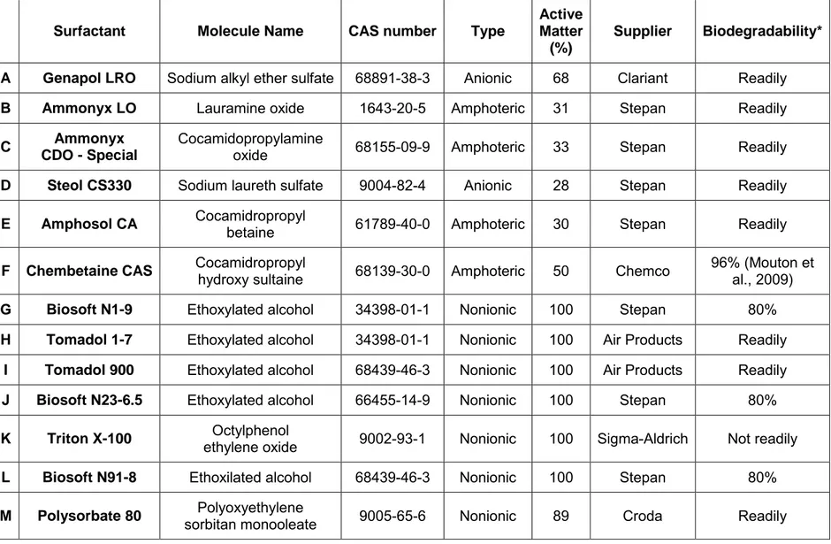
Three criteria were considered in order to select the most suitable surfactant for foam production; biodegradability, foamability and interfacial tension. Foamability was measured with the Ross Miles Test (ASTM D1173). Interfacial tensions between surfactants and p-xylene were measured by the pendant drop method (Woodward, 2011). Table 3.1 presents the list of all tested surfactants including their biodegradability. They are all biodegradable, except for Triton X-100 which was tested for comparison purposes

Table 3.1 – List of tested surfactants.

Surfactant Molecule Name CAS number Type

Active Matter

(%)

Supplier Biodegradability*

A Genapol LRO Sodium alkyl ether sulfate 68891-38-3 Anionic 68 Clariant Readily

B Ammonyx LO Lauramine oxide 1643-20-5 Amphoteric 31 Stepan Readily

C Ammonyx

CDO - Special

Cocamidopropylamine

oxide 68155-09-9 Amphoteric 33 Stepan Readily

D Steol CS330 Sodium laureth sulfate 9004-82-4 Anionic 28 Stepan Readily

E Amphosol CA Cocamidropropyl _betaine 61789-40-0 Amphoteric 30 Stepan Readily

F Chembetaine CAS Cocamidropropyl _{hydroxy sultaine} 68139-30-0 Amphoteric 50 Chemco 96% (Mouton et _{al., 2009)}

G Biosoft N1-9 Ethoxylated alcohol 34398-01-1 Nonionic 100 Stepan 80%

H Tomadol 1-7 Ethoxylated alcohol 34398-01-1 Nonionic 100 Air Products Readily

I Tomadol 900 Ethoxylated alcohol 68439-46-3 Nonionic 100 Air Products Readily

J Biosoft N23-6.5 Ethoxylated alcohol 66455-14-9 Nonionic 100 Stepan 80%

18

Foamability

The Ross Miles Test (ASTM D1173 method) quantifies both the capacity to produce foam and its stability under standardized conditions. This method is used to compare surfactants that produce foam, it does not measure any intrinsic property and needs to be used under the same conditions for all tests. All surfactants were tested at these concentrations: 0.01%, 0.1% and 1% w/w.

A standard apparatus is needed to carry out the Ross Miles Test (Figure 3.1). This apparatus consists of a glass receiver and a 200 ml glass pipet (Wilmad LabGlass, New Jersey). The methodology is as follows: (1) the walls of the receiver are rinsed with distilled water in order to clean any remaining surfactant; (2) the stopcock at the bottom of the receiver is closed and the walls are rinsed with 50 ml of the surfactant solution, which remains at the receiver bottom; (3) the pipet is placed on top of the receiver. The receiver height is standardized so the bottom of the pipet is exactly at a 90 cm height of the 50 ml line; (4) the pipet stopcock is opened, which allows the surfactant solution to fall into the 50 ml of surfactant solution already at the bottom of the receiver; (5) foam is produced by the solution’s drop; (6) when all the solution has run out, a measurement of foam height is taken at t=0 min and a stopwatch is started and further measurements are taken at times of 1, 3, 5 and 15 minutes.

This method has the following advantages: each test is done in a short period of time, it is repeatable and the apparatus height allows neglecting the effect of humidity. As reported by Li et al. (2012b), the distance between the top of the foam and the receiver top opening is crucial for the humidity gradient over the foam, which has an effect on foam collapse. When the humidity gradient is low, the evaporation rate is also low and the foam is more stable.

Considering that the best foam tested reached a height of 18.6 cm and the receiver total height of 90 cm, a distance of 71.4 cm was considered sufficient to have negligible evaporation. However, this technique does not consider the change in foam quality through time, only the foam height. Therefore, even if most of the liquid contained initially in the foam has drained out and the bubbles are large and unstable, foam height can still remain the same as initially measured. Bubbles can collapse and all the liquid is drained down or bubbles can join and form bigger bubbles that will remain in place. Therefore, measurements of foam height through time are not good indications of foam stability; thus measurements through time were not considered for the present study.

Sometimes, bubbles become bounded to the glass walls and create a higher concentration of bubbles near the walls that stabilize them. A hole in the middle of the receiver is apparent. When it occurred, measurements of foam height were made where it appeared continuous through the width of the receiver.

Interfacial tension

Interfacial tensions between surfactant solution and p-xylene were measured with a FTA 200 Dynamic Contact Angle Analyzer from First Ten Angstroms, which uses the pendant drop technique. Images are taken of a p-xylene drop injected upside down with a “U” shaped flat ended needle (0.356 mm diameter) in a glass cell filled with the tested surfactant at concentrations of 0.01%, 0.1% and 1%. A computer activated pump controls p-xylene injection. A p-xylene drop needs to be large enough to be distorted by gravity as interfacial tension tries to balance this distortion. Interfacial tension (IFT) is assessed by fitting the shape of the drop to the

20

3.2.2 Foam production and injection system

Many foam production methods were tested, including: injection at constant rate with syringe pumps, injection with a porous stone in a foam production column and alternating injection of surfactant and air at the same pressure in a foam production column. The first two methods did not perform well because no foam was produced by either method. Indeed, when tested in the laboratory, these methods only produced alternate slugs of air and surfactant solution. The latter method was selected because a constant flow of foam was easily produced and foam quality was easily measurable. Furthermore, foam production at a constant pressure has been reported to be more efficient than production at a constant rate (Li, 2011).

A stainless steel tank (6.6 L, 18 cm diameter, 26 cm height, 5 mm thick) was filled with surfactant solution and connected to the pressurized air line controlled by a pressure regulating valve (0.64 cm diameter, 300 psi, Parker) (Figure 3.2). Then, both air and surfactant solution lines were connected to two valves (0.5 cm diameter, shutoff valve 104R, Asco) that opened alternatively at fixed times steps. This setup allowed air and surfactant solution injection at the same pressure.

After initial tests, it appeared that alternating times had no significant effect on foam production, so it was decided that fixed times were to be used for all further testing: five seconds of surfactant solution injection alternating with ten seconds of air injection. Those short periods of time were selected because they created only small variations in the injection pressure signal and thus in the pressure transducer response. Also, heating of the electric valves favored short alternate opening of each valve. After flowing through the valves, air and surfactant solution are mixed in a ‘’T’’ shaped tube and then go through a foam production column, which is an acrylic column filled with 2 mm diameter glass beads with 250 μm opening screens between each 2.5 cm glass bead layers. This column allowed the purging of foam until it was stable and the measurement of its quality before it entered the sand column. This procedure only allowed already pressurized stable foam to enter the sand column.

When foam exiting the production column had a stable quality, it was flowed through the glass sand column and filmed at a high resolution with a digital camera (Nikon, Coolpix P510). As shown on Figure 3.2, four pressure transducers were also placed at key positions throughout the system, to measure changes in pressure along the production system: one at the foam production column inlet (T-1), one at the sand column inlet (T-2), one in the upper and lower ports in the sand column (T-3 and T-4). The line carrying the effluent was placed at a fixed

height of 5 cm above the sand column inlet to maintain a back pressure at the outlet of the column. The next section further describes sand column experiments.

Figure 3.2 - Experimental setup for foam production and injection into sand columns. T-1 through T-4 refer to pressure transducers. Videos were made of foam flow through the transparent acrylic sand column.

3.2.3 Sand column experiments

Sand column experiments are a first step towards the assessment of the suitability of foam for LNAPL remediation, prior to laboratory sand box experiments and field pilot-testing. Sand column tests were designed to help understand the effects of different variables on foam flow through soils, especially pre-column use, injection pressure, surfactant concentration, pre-flush liquid and surfactant types. Sand column experiments were done with the three more suitable surfactants selected following foamability tests and interfacial tension measurements described previously.

Silica sand (99.9% quartz) was used for all experiments in order to minimize fines (clay and silt) and organic matter contents of soils and the interaction of surfactant with other minerals. The same silica sand was used for all tests, which was Temisca 20 (Opta Minerals Inc.), a coarse sand whose properties are listed in Table 3.2.

Table 3.2 – Properties of Temisca 20 sand used in column experiments. d10 and d50 refer to grain sizes larger

22

14.5 cm length. Acrylic was selected for its resistance to compression and its transparency, which allowed the filming of foam flow. Both ends are sealed with a perforated Teflon cap combined with a reservoir that uniformly distributes fluids before their entry into the sand column. The seal between the acrylic cylinder and the Teflon caps is provided by a Viton O-Ring. A nylon screen (125 μm mesh) on each Teflon cap prevents the loss of sand through the perforated caps. Two holes were pierced on the side of the column to connect pressure transducers and the same nylon screen was placed on each hole to prevent sand loss.

Compaction of each 5 mm sand layers was done by dropping a 500 g weight 12 times from a height of 8 cm. The top surfaces of compacted layers were lightly scarified to minimize preferential flow paths between subsequent layers. The sand column had a global dry density of 1.64 g/cm³ which is enough to prevent channeling that may occur below 1.6 g/cm³ (Ripple et al., 1973). Trapped air in column was eliminated by circulating at least 30 pore volumes of CO2 through the column. Then the column was saturated from the bottom up with degased distilled water in which CO2 solubilizes. At least 3 pore volumes (PV) of water were circulated through the sand column in order to flush or solubilize all CO2. The same column was used for every tests mentioned in this study in order to produce comparable experiments. After each test, the column was rinsed with water and dried with compressed air. It was then purged with CO2 and saturated again with degassed distilled water.

The effects of four conditions were tested in column: the use of a foam production column, pre-flush with surfactant or water, the use of different solubilized surfactants and the injection pressure.

The effect of the foam production column was tested by making two tests: one with a foam production column and one without. Both tests were done with the same conditions except that one test was done without a foam production column. This test was done as follows: pressurized surfactant was injected first and then air was injected in the sand column after the completion of surfactant solution injection. So, in this test, foam was produced inside the column whereas it was produced in the foam production column in the other test. The effect of the pre-flush liquid was tested by making two tests: one with a column pre-pre-flushed with water and one with a column pre-flushed with surfactant prior to foam injection. Both tests were done with the same foam injection conditions. The effect of the use of different surfactants was tested by making three tests, each with a different surfactant solution chosen following Ross Miles test and Pendant Drop test results. These three tests were done with the same foam injection conditions. The effect of injection pressure was tested by making two tests: one at a lower

injection pressure and another with a higher injection pressure. Other than injection pressure, both tests were done with the same foam injection conditions.

Foam apparent viscosity measurements were done for each column test in order to evaluate the effect of each parameter previously mentioned. They were estimated via foam flow rate and pressure measurements. Injection pressure was fixed for each test and pressure throughout the setup was measured with pressure transducers (T-1 through T-4) positioned as shown in Figure 3.2. Flow rate was calculated with two indirect methods: the velocity of the foam front (Front Velocity Method) and the foam flow rate at the system outlet (Output Method). The Front Velocity Method involved the measurement of the foam front velocity when it passed the second pressure transducer in the column. Apparent viscosity was calculated using the pressure gradient between the two pressure transducers (T-3 and T-4) in the column at that time. This method provides an evaluation of foam viscosity at the beginning of the column test, before the column is completely swept by foam. The Output Method used foam rate measured at the column outlet after a certain time of foam injection, when the pressures measured in the column had stabilized. For this method, apparent viscosity was calculated using the stabilized pressure gradient between the two pressure transducers (T-3 and T-4) in the column and the measured flow rate at the column outlet. This method provides a stabilized measurement of foam viscosity at the end of the experiment.

3.3 Results

3.3.1 Surfactant selection

Foamability

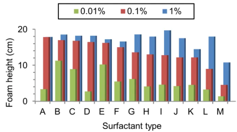
Figure 3.3 presents foamability indicated by the initial foam height of the Ross Miles Test for all surfactants tested. Surfactants have been placed in decreasing order starting from the best to worst foamability at 0.1% surfactant concentration (red columns). Considering the small changes in foamability between concentrations of 1% and 0.1% for the best surfactant

24

Figure 3.3 –Foamability of surfactant solution at concentrations of 0.01%, 0.1% and 1% measured with the Ross Miles Test for all tested surfactants (A through M; see Table 3.1).

Interfacial tension

Interfacial tension is a key parameter for the evaluation of potential NAPL dissolution and mobilization. In order to maximize the capillary number for mobilization, the interfacial tension between the NAPL and surfactant solution has to be minimized. Figure 3.4 shows interfacial tensions between p-xylene and the surfactant solutions tested. Surfactants were placed in order of increasing interfacial tension at a 0.1% w/w concentration. Surfactant B would provide the best mobilization because it lowers interfacial tension with the NAPL by two orders of magnitude compared with water.

Figure 3.4 - Interfacial tension between p-xylene and the tested surfactant solutions at concentrations of 0.01%, 0.1% and 1% (A through M; see Table 3.1Table 3.1).

Considering pendant drop and Ross Miles test results, three surfactants (A, B, and, I) were selected to be further studied in column tests (Figure 3.5 and 3.7). Surfactant A has the best foamability but has an interfacial tension with p-xylene higher than surfactant B, which shows

0 10 20 A B C D E F G H I J K L M Surfactant type F oa m he igh t (c m ) 0.01% 0.1% 1% 0 8 16 B F C E M A D G H L K J I Surfactant type Int erf ac ial ten si on ( m N/m ) 1% 0.1% 0.01%

the lowest interfacial tension. Surfactant I presents worse results in both tests than the other two surfactants, but it was selected to provide a comparison of the performance that can be obtained with a poor foaming agent. Considering those comparisons, surfactant B was expected to be the best surfactant for p-xylene remediation purposes. Surfactant B was thus selected to carry out for p-xylene remediation purposes. Surfactant A and B were thus selected to carry out column tests aiming to show the influence of different conditions.

Figure 3.5 - Foamability expressed as foam height (cm) of selected surfactant solutions measured with the Ross Miles Test at three different times at 0.1% concentration.

18 ₁₇ 13 15 15 11 15 13 6 0 10 20 A B I F oa m he igh t (c m ) Surfactant 0 min 3 min 15 min 3.4 0.7 2.0 4.7 0.8 9.2 15 5 16 0 10 20 A B I Int erf ac ial ten si on ( m N/m ) Surfactant 1% 0.1% 0.01%

26

3.3.2 Sand column tests for the effect of various conditions

Several tests were carried out to compare the effect of various conditions on foam flow in a sand column: the effect of foam production column use, pre-flush liquid, surfactant solution used and injection pressure. Table 3.3 summarizes all types of columns tests carried out in this study. Table 3.4 summarizes which column tests were used to evaluate each parameter studied in this work.

Table 3.3 – Summary of column tests including the characteristics of each test, a concentration of 0.1% w/w was used for all tests.

Test Number Foam production column Pre-flush Liquid* Surfactant Injection pressure (cm H2O) 1 Yes SS A 350 2 No SS A 350 3 Yes SS B 350 4 Yes W B 350 5 Yes SS I 350 6 Yes SS B 210

* SS stands for surfactant solution and W for water.

Table 3.4 – Summary of the conditions evaluated with the corresponding column tests and figures.

Parameter evaluated Figure Tests compared

Effect of foam production column presence Figure 3.7 1 2 Pre-flush with water or surfactant Figure 3.9 3 4 Use of surfactant solution A, B or I Figure 3.12 1 3 5

Injection pressure Figure 3.14 3 6

Effect of a foam production column on foam stability

This test was done to verify if the use of a foam production column before the injection of foam in the porous media (represented by a sand column) may increase the foam apparent viscosity. So, a test was done with (Test 1) and without (Test 2) a foam production column. Since foam is injected at the same pressure (350 cm water) in both cases, viscous foam will advance more slowly in the column. Photos of the advancing foam front are shown in Figure 3.7 and it clearly indicates the velocity (and thus viscosity) of the injected foam.

Figure 3.7 - Advancing foam front of surfactant A (0.1% w/w concentration) injected downward following a surfactant pre-flush at a constant pressure of 350 cm water in a Temisca 20 sand column with and without a foam production column. The black dotted line indicates the foam front position. Figure 3.7 indicates that the front in the test without a foam production column (top) moved significantly faster than in the test with a foam production column (bottom). This thus indicates a greater foam viscosity when a foam production column is used compared to the test without foam production column. Both experiments involved the formation of a strong foam with a stable water displacement front. Evaluation of viscosity with the Front Velocity method indicated a value of 8 mPa∙s without a foam production column and 338 mPa∙s with it (Figure 3.8). When the foam front passed the second pressure transducer, it was a lot more viscous in Test 1 than

Foam F lo w d irec tion 14.5 cm 3.5 cm S urf ac tan t A Foam S urf ac tan t A

28

Considering these results, the following tests were done with a foam production column in order for the foam to stabilize more quickly and be more viscous.

Figure 3.8 – Calculated foam viscosity (mPa∙s) of foam produced with 0.1% concentration surfactant A solution in sand column with and without a foam production column using the Front Velocity and Output methods.

Effect of water or surfactant pre-flush

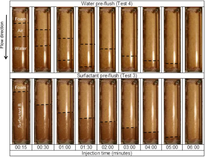
The sand column must be pre-flushed with a liquid prior to foam injection to be representative of saturated conditions as found in the field. Two scenarios with water (Test 4) and surfactant solution (Test 3) as pre-flush liquid were tested with surfactant B at a concentration of 0.1% and a foam injection pressure of 350 cm H2O in the sand column.

Figure 3.9 shows that, with surfactant pre-flush, a straight uniform front formed, indicating the formation of a strong foam. For the water pre-flush experiment, there is formation of a first blurred foam front with poor sweep and then a second front with more viscous foam that advances more slowly and with better sweep efficiency. However this second front and the front observed in surfactant pre-flush experiment take the same time to sweep entirely the column, thus indicating that foam viscosity is similar. In order to evaluate apparent viscosity with the Front Velocity Method in the sand column test with water pre-flush, the second front which was more clearly defined was selected. Figure 3.10 shows the apparent foam viscosities estimated with the Front Velocity and Output methods, which confirm that foam viscosity was almost identical with the two types of pre-flush fluids.

338 8 254 204 0 200 400

with foam production

column no foam productioncolumn

V is co si ty ( m P a∙s )

Front Velocity method Output method

Figure 3.9 - Advancing foam front of surfactant B injected downward at a pressure of 350 cm H2O in the sand column pre-flushed with water or liquid surfactant as a function of time (minutes). The black dotted line indicates the foam front position.

40 54 44 59 50 100 V is co si ty ( m P a∙s )

Front Velocity method Output method

Foam Water Air Foam S urf ac tan t B F lo w d irec tion

30

Figure 3.11 shows each front velocity through time before they attained the column outlet. The second front with water pre-flush and the front with surfactant pre-flush both show similar advancing behavior which indicate similar viscosities as injection pressure was stable throughout the experiments. Viscosities calculated with both methods are similar for both tests (Figure 3.10). They indicate that pre-flush with water or surfactant solution does not significantly affect foam viscosity. Therefore, it was decided that all further experiments would be done with a surfactant pre-flush in order to create an easily observable and stable foam front.

Figure 3.11– Foam front velocity of surfactant B solution 0.1% foam injected in Temisca 20 sand column pre-flushed with water or surfactant solution B 0.1%.

Effect of surfactant type

Figure 3.12 compares the position of foam fronts for 0.1% concentrations of surfactants A (Test 1), B (Test 3) and I (Test 5) injected at pressures of 350 cm of water in the sand column. It shows that surfactant I has a foam front much faster than the two others; the slowest being surfactant A. Also, the front becomes unstable at the end of foam injection in sand column with surfactant solutions A and I.

Figure 3.13 shows the estimated viscosities of these foams. Surfactant A is the most viscous and is followed by surfactant B and surfactant I. Therefore, the ranking of surfactants based on the foamability with the Ross Miles Test (Figure 3.5) is respected, which indicates that this simple test can provide representative indications on surfactant foamability in columns. However, surfactant A produced foam so viscous that the pressure gradient in the column was too large and the front became unstable before the complete sweep of the column (Figure 3.12).

0.0 1.0 2.0 00:00 02:30 05:00 F ron t po si tion ( cm ) Time (mm:ss)

Foam front with solution B preflush 1st foam front with water preflush 2nd foam front with water preflush

Foam viscosity even dropped during the pressure stabilization in the column, which explains the drop between the two calculations of viscosity in Figure 3.13. Based on these results, it was decided that surfactant B would be used for further testing.

Foam S urf ac tan t I F lo w d irec tion Foam S urf ac tan t A Foam S urf ac tan t B

32

Figure 3.13 - Calculated foam viscosity in Temisca 20 sand column injected with surfactants A, B and I.

Effect of injection pressure

Further column tests were done with surfactant B solution at a concentration of 0.1% at two different injection pressures: 210 cm H2O (Test 6) and 350 cm H20 (Test 3). These tests aimed to determine if a lower injection pressure, more suitable for field conditions, could be used and still maintain foam stability and viscosity. An injection pressure of 350 cm H2O produces a significantly more viscous and more stable foam front than injection at 210 cm H2O (Figure 3.14). Moreover, a higher injection pressure produces foam that stabilizes and gains viscosity through time as shown in Figure 3.15 by the increasing gap between viscosities estimated at the beginning of the test with the Front Velocity method and at the end of the test with Output method. 338 54 5 254 59 10 0 200 400 A B I V is co si ty ( m P a∙s ) Surfactant

Front Velocity method Output method

Figure 3.14 - Advancing foam front of surfactant B solution 0.1% injected downward at pressures of 210 and 350 cm H2O in the sand column pre-flushed with surfactant B solution as a function of time

(minutes). The black dotted line indicates the foam front position.

54 59 50 100 V is cos ity ( m P a∙s ) Front Velocity method Output method Foam S urf ac tan t B Foam S urf ac tan t B F lo w d irec tion