EVALUATION OF HYDROLOGICAL ENSEMBLE
PREDICTION SYSTEMS FOR OPERATIONAL
FORECASTING
Thèse présentée
à la Faculté des études supérieures de l'Université Laval dans le cadre du programme de doctorat en Génie civil pour l'obtention du grade de Philosophiae Doctor (Ph.D.)
DEPARTEMENT DE GENIE CIVIL ET GENIE DES EAUX FACULTÉ DES SCIENCES ET DE GÉNIE
UNIVERSITÉ LAVAL QUÉBEC
2010
La prévision hydrologique consiste à évaluer quelle sera l'évolution du débit au cours des prochains pas de temps. En utilisant les systèmes actuels de prévisions hydrologiques déterministes, il est impossible d'apprécier simplement l'incertitude associée à ce type de prévision, ce que peut nuire à la prise de décisions.
La prévision hydrologique d'ensemble (PHE) cherche à étayer cette incertitude en proposant, à chaque pas de temps, une distribution de probabilité, la prévision probabiliste, en place et lieu d'une estimation unique du débit, la prévision déterministe.
La PHE offre de nombreux bénéfices : elle informe l'utilisateur de l'incertitude; elle permet aux autorités qui prennent des décisions de déterminer des critères d'alerte et de mettre en place des scénarios d'urgence; elle fournit les informations nécessaires à la prise de décisions tenant compte du risque.
L'objectif principal de cette thèse est l'évaluation de prévisions hydrologiques d'ensemble, en mettant l'accent sur la performance et la fiabilité de celles-ci. Deux techniques pour construire des ensembles sont explorées: a) une première reposant sur des prévisions météorologiques d'ensemble (PME) et b) une seconde exploitant simultanément un ensemble de modèles hydrologiques (multimodèle).
En termes généraux, les objectifs de la thèse ont été établis afin d'évaluer :
a) les incertitudes associées à la structure du modèle : une étude qui repose sur des simulations journalières issues de dix-sept modèles hydrologiques globaux, pour plus de mille bassins versants français;
b) les incertitudes associées à la prévision météorologique : une étude qui exploite la PME du Service Météorologique du Canada et un modèle hydrologique opérationnel semi-distribué, pour un horizon de 3 jours sur douze bassins versants québécois;
c) les incertitudes associées à la fois à la structure du modèle et à la prévision météorologique : une étude qui repose à la fois sur la PME issue du ECMWF (European
Centre for Medium-Range Weather Forecasts) et seize modèles hydrologiques globaux, pour un horizon de 9 jours sur 29 bassins versants français.
Les résultats mets en évidence les avantages des systèmes probabilistes par rapport aux les déterministes. Les prévisions probabilistes sont toutefois souvent affectées par une sous dispersion de leur distribution prédictive. Elles exigent alors un post traitement avant d'être intégrées dans un processus de prise de décision. Plus intéressant encore, les résultats ont également montré le grand potentiel de combiner plusieurs sources d'incertitude, notamment celle associée à la prévision météorologique et celle associée à la structure des modèles hydrologiques. Il nous semble donc prioritaire de continuer à explorer davantage cette approche combinatoire.
Abstract
Hydrological forecasting consists in the assessment of future streamflow. Current deterministic forecasts do not provide information concerning the uncertainty, which might be limiting in a decision-making process.
A hydrological ensemble prediction system (H-EPS) seeks assessing the uncertainty of the forecast by proposing an ensemble of possible forecasts, from which one can estimate the probability distribution of the predictand at each time step (the probabilistic forecast), instead of the usual single flow estimate (the deterministic forecast).
A H-EPS offers many benefits: it informs the user about the uncertainty and it allows decision-makers to determine criteria for alarms based on the probability of exceeding certain thresholds and to test emergency measures on the scenarios proposed by the H-EPS. In short, it allows users to manage the risk associated with decisions based on a forecast. The main scope of this thesis is the evaluation of H-EPS for operational forecasting, with emphasis on performance and reliability. Two techniques to construct ensembles are explored: a) a system based on a meteorological ensemble prediction system (M-EPS) coupled with an operational hydrological model and b) a system based on multimodel hydrological ensembles.
In general terms, the objectives of the thesis are designed to assess the uncertainty in different cases:
a) Uncertainties associated with model structure: analysing daily simulation over a thousand French catchments and 17 lumped model structures.
b) Uncertainties from the meteorological forecasting: assessing Meteorological Service of Canada M-EPS and short-term hydrological forecasts issued from a distributed model, over 12 catchments located in the Province of Québec and a 3-day horizon.
c) Uncertainties from both hydrological model and forcing inputs: exploring 16 lumped hydrological model structures driven by daily ensemble predictions issued by the
European centre for medium-range weather forecasts M-EPS, over 29 French catchments and a 9-day horizon.
Results confirmed the added value of probabilistic systems over currently used deterministic systems. However, in many instances, the lack of reliability asks for post processing of the predictive distribution.
Results also stressed the advantage of simultaneously dealing with the many sources of uncertainty of hydrological predictions: a promising path for further research.
Je tiens tout d'abord à remercier François Anctil, pour avoir dirigé ma recherche, pour le suivi de mon travail au Québec et en France, son encouragement, ses conseils et sa disponibilité en tout temps.
Mes sincères remerciements à l'unité Hydrologie des bassins versants du Cemagref (Antony, France) où j'ai effectué un stage de recherche de six mois. Un merci particulier à Vazken Andréassian pour son chaleureux accueil et pour avoir gracieusement partagé la base de données des bassins versants français. J'adresse aussi ma gratitude à Charles Perrin, pour l'accès aux 17 modèles globaux et à Maria-Helena Ramos pour avoir préparé les données de prévision d'ensemble d'ECMWF. Merci pour les critiques constructives et la rigueur scientifique qui m'ont beaucoup aidé pour améliorer la qualité de ma recherche et les manuscrits soumis.
Merci à Richard Turcotte du Centre d'expertise Hydrique du Québec pour les données hydrométéorologiques et à Vincent Fortin d'Environnement Canada pour les données du système de prévision d'ensemble nécessaires à la recherche sur les bassins versants du Québec. Merci aussi pour tous les commentaires constructifs pendant la préparation du manuscrit qui a été finalement publié dans HESS.
Merci aux professeurs du Département de génie civil et génie des eaux, en particulier à Geneviève Pelletier, Brian Morse et Peter Vanrolleghem pour le suivi et commentaires lors mes séminaires de recherche. Merci à Noël Evora et Jean-Loup Robert pour leur disposition comme jury lors de mon examen doctoral. Je voudrais aussi remercier à Richard Turcotte, Vincent Fortin et Brian Morse pour avoir accepté d'être membres de jury de ma thèse.
Je voudrais aussi remercier mes collègues et amis du Département de génie civil et génie des eaux, tout spécialement Marie-Amélie Boucher, pour avoir partagé avec enthousiasme son expertise sur les prévisions d'ensemble, Thomas Petit, qui
m'a beaucoup aidé avec le modèle Hydrotel et Audrey Lavoie avec qui j'ai travaillé pour faire tourner ces simulations et.
Merci à l'organisme boursier CONACYT (Consejo Nacional de Ciencia y Tecnologia de Mexico) et à la Chaire de Recherche EDS en Prévisions et Actions Hydrologiques (CRPAH) pour l'appui financier.
J'adresse finalement tout ma gratitude à mes amis de Québec et de Paris, avec lesquels j'ai partagé de bons moments tout au long de ces trois années.
Merci à ma famille pour son soutien inconditionnel. Encore une fois, merci à tous.
En perseguirme, Mundo, iqué interesas? cEn que te ofendo, cuando solo intento poner bellezas en mi entendimiento y no mi entendimiento en las bellezas?
Yo no estimo tesoros ni riquezas; y asi, siempre me causa màs contento poner riquezas en mi pensamiento que no mi pensamiento en las riquezas. Y no estimo hermosura que, vencida, es despojo civil de las edades, ni riqueza me agrada fementida, teniendo por mejor, en mis verdades, consumir vanidades de la vida que consumir la vida en vanidades. SorJuana Inès de la Cruz (1651-1695)
Table of contents
Résumé i Abstract iii Remerciements v Table of contents ix Liste of symbols xi Liste of tables xii Liste of figures xiiiChapter 1. Introduction and Objectives 1 1.1 Meteorological Ensemble Prediction System 3
1.1.1 The ECMWF and MSC Ensemble Prediction Systems 4
1.2 Hydrological Ensemble Prediction System 5
1.2.1 Operational H-EPS 8 1.2.2 The Multimodel Ensemble 10
1.2.3 Combining Multimodel and EPS techniques 13
1.3 Objectives of the research 15 1.3.1 Objective 1: Evaluation of multimodel ensemble simulation 15
1.3.2 Objective 2: Evaluation of the Canadian global M-EPS for short-term H-EPS 16 1.3.3 Objective 3: Evaluation of a multimodel ensemble hydrological prediction
system 17 1.4 Organization of the thesis 18
Chapter 2. Methodology for evaluating probabilistic forecasts 19
2.1 Performance evaluation 20 2.1.1 The Absolute Error criteria 20 2.1.2 The Continuous Ranked Probability Score 21
2.1.3 The rank histogram 23
2.1.3.1 Ratio Ô 25 2.1.4 The reliability diagram 26
2.1.5 Hit over threshold criteria 27 2.2 Post processing methods. 29 Chapter 3. Evaluation of multimodel ensemble simulation 30
3.1 Data and hydrological models 31
3.1.1 Catchments 31 3.1.2 Hydrological Lumped Models 31
3.2 Experimental setup 34 3.2.1 Genetic algorithm 34
3.3 Results 37 3.3.1 Individual model performance 37
3.3.2 Deterministic and probabilistic performance 37
3.3.3 Reliability 40 3.3.4 Hit over threshold criteria 43
Chapter 4. Evaluation of the Canadian global Meteorological Ensemble Prediction
System for short-term hydrological forecasting 50
4.1 Data and models 51 4.1.1 Meteorological forecasting 51
4.1.2 Hydrological Forecasting 51 4.1.3 Watershed description 52 4.2 Experimental setup 55
4.3 Results 58 4.3.1 Deterministic and probabilistic performance 58
4.3.2 Reliability 59 4.4 Summary 65 Chapter 5. Evaluation of a Multimodel Ensemble Hydrological Prediction System 67
5.1 Data and models 68 5.1.1 Catchments 68 5.1.2 Rainfall forecasts from ECMWF 69
5.1.3 Hydrological Lumped Models 70
5.2 Experimental setup 72
5.3 Results 73 5.3.1 Performance and reliability of the ECMWF-EPS 73
5.3.2 Individual model performance 75 5.3.3 Deterministic and probabilistic performance 75
5.3.4 Reliability 76 5.3.5 Hit over threshold criteria 79
5.4 Summary 80 Chapter 6. Conclusion 82
List of symbols
5= ratio delta
A= ratio for a given ensemble
A0= ratio for a perfectly reliable system
C0= reference ensemble obtained by pooling all seventeen lumped model outputs. Cl= ensemble of the best eight individual models
C2= ensemble of the worst eight individual models Coptim-ensemble obtained with the optimisation procedure
CRPS = mean Continuous Ranked probability Score CRPSref= reference Continuous Ranked probability Score £=expected value
Ft = cumulative predictive distribution function. H= Heaviside function
K = a given interval of the rank histogram. MAE= mean absolute error
n = members of the ensemble
«*= selected random members of the ensemble. N= number of ranks of the rank histogram POD= probability of detection
POFD= probability of false detection
ROC= relative operating characteristic curve
Sk= number of elements of the h!h interval of the rank histogram
SSCRPS= skill score of CRPS t= time
x= predicted variable x,= observed value
Liste of tables
Table 1. Examples of operational and pre-operational flood forecasting systems using ensemble weather predictions as inputs, from Cloke et al. (2009).
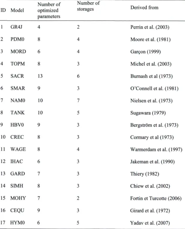
Table 2. Contingency table for a dichotomous event. Table 3. Characteristics of the 1061 catchment dataset. Table 4. Models identification and characteristics. Table 5. Streamflow data analyzed.
Table 6. Main characteristics of the studied catchments. Table 7. Models identification and characteristics.
Table 8. Scenarios of hydrological ensemble predictions (H-EPS) tested in this study, based on 16 hydrological models, and deterministic (ECMWF-DPS) and probabilistic (ECMWF-EPS) rainfall forecasts.
Liste of figures
Fig. 1 Description of the CRPS for a) a given observed variable and the hypothetical probability density functions of its ensemble forecast b) cumulative density function of observed variable and ensemble forecast c) cumulative density function of observed variable and its deterministic forecast.
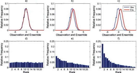
Fig. 2. Hypothetical probability density functions for a given observed variable and its ensemble prediction along with their associated rank histograms for: (a) under dispersed pdf, (b) well calibrated pdf, and (c) over dispersed pdf, (d) rank histogram corresponding to (a), (e) rank histogram corresponding to (b) and (f) rank histogram corresponding to (c).
Fig. 3. Hypothetical probability density functions for a given observed variable and its ensemble prediction along with their associated rank histograms, (a) well calibrated pdf, (b) and (c) represents different degrees of bias in the pdf, (d) rank histogram corresponding to (a), (e) rank histogram corresponding to (b) and (f) rank histogram corresponding to (c).
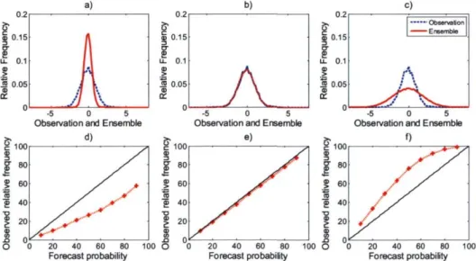
Fig. 4. Hypothetical probability density functions for a given observed variable and its ensemble prediction along with their associated reliability diagrams for: (a) under dispersed pdf, (b) well calibrated pdf, (c) over dispersed pdf, (d) reliability diagram corresponding to (a), (e) reliability diagram corresponding to (b) and (f) reliability diagram corresponding to (c).
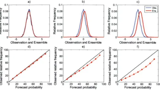
Fig. 5. Hypothetical probability density functions for a given observed variable and its ensemble prediction along with their associated reliability diagrams, (a) well calibrated pdf, (b) and (c) represents different degrees of bias in the pdf, (d) reliability diagram corresponding to (a), (e) reliability diagram corresponding to (b) and (f) reliability diagram corresponding to (c).
Fig. 6. Example of relative operating characteristic (ROC) curve.
Fig. 7. Location of the 1061 gauging stations and corresponding catchment boundaries (Le Moine, 2008).
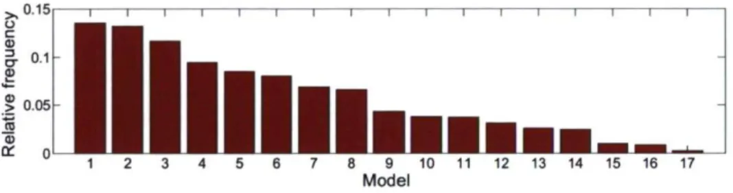
Fig. 8. Relative frequency of occurrence in the top 5 ranking, based on individual MAE values for all catchments.
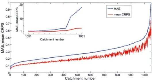
Fig. 9. Mean probabilistic and deterministic scores comparison. Catchments are ordered according to their MAE value.
Fig. 10. Mean deterministic scores comparison (MAE of the ensemble and MAE of the best individual model). Catchments are ordered according to the value of the MAE of the ensemble.
Fig. 11. Relative frequency of occurrence as the best model or ensemble: a) deterministic (MAE) andb) probabilistic (CRPS).
Fig. 12. Six examples of rank histograms with their ratio Ô values.
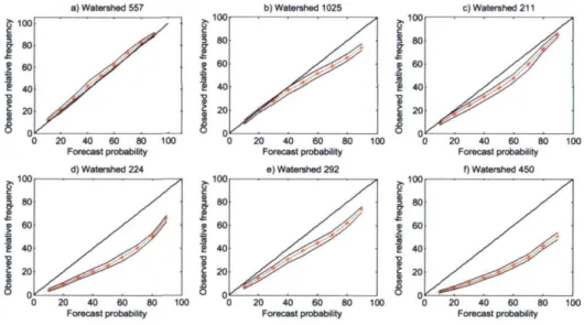
Fig. 13. Reliability plots for the same catchments as in Figure 12, for all time series. Dashed lines depict the 95% confidence interval.
Fig 14. Reliability plots for the same catchments as in Figure 12, for discharge larger than quantile 50 of the observation time series. Dashed lines depict the 95% confidence interval.
Fig. 15. Reliability plots for the same catchments as in Figure 12, for discharge larger than quantile 75 of the observation time series. Dashed lines depict the 95% confidence interval.
Fig. 16. Cumulative frequency of ratio Ô for the CO reference ensembles.
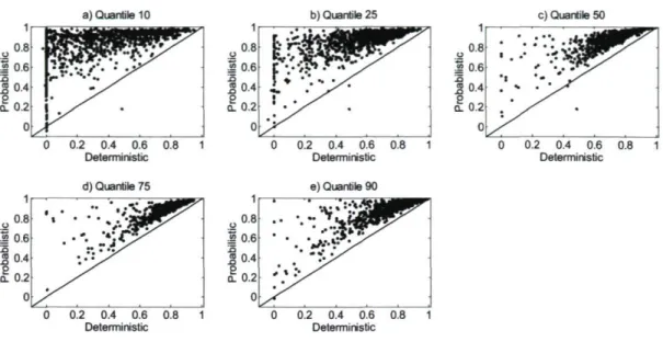
Fig. 17. Probabilistic and deterministic ROC scores for quantiles 10, 25, 50, 75 and 90. Fig. 18. Cumulative frequency of the CRPS gain after optimization.
Fig. 19. Scatter plot ratio ô values without (CO) and with optimization.
Fig. 20. Relative frequency of a) the presence of each model in the optimized subset, and b) the number of models in these subsets, for all 1061 catchments.
Fig. 21. Box plot of the CRPS over the 1061 catchments, as a function of the number of models per optimized subsets. The box has lines at the lower, median, and upper quartile values (IQR) and whiskers extend to 1.5xIQR.
Fig.22. Examples of rank histograms for a given catchment with ensembles CO, Cl, C2 and the optimized subset Coptim.
Fig. 23. Localization of the five selected river systems (Province of Québec, Canada). Fig. 24. Precipitation and standardized streamflow observations from 11 to 31 October
2007.
Fig. 25. H-EPS mean probabilistic and deterministic score comparison as a function of the prediction horizon.
Fig. 26. H-EPS Rank histograms after 100, 200 and 400 bootstrap repetitions: ChaudièreT6 watershed, 72-h horizon.
Fig. 28. H-EPS 72-h rank histograms.
Fig. 29. H-EPS 24-h, 48-h, and 72-h reliability diagrams: Chaudière T6 watershed. Fig. 30. H-EPS 72-h reliability diagrams.
Fig. 31. MSC-EPS Ratio ô as a function of the prediction horizon.
Fig. 32. H-EPS 72-h reliability diagrams. Case 1 evaluates the reliability of an updated flow forecasting against the observed discharge. Case 2 evaluates a no-updated forecast against the base line simulation.
Fig. 33. Location of the 29 studied catchments in France.
Fig. 34. Mean SSCRPS of the ECMWF-EPS as a function of lead time for the 29 studied
catchments.
Fig 35. Reliability Diagrams of the ECMWF-EPS for the 29 studied catchments and lead times of a) 1 day, b) 2 days, c) 3 days, d) 5 day, e) 7 days, f) 9 days.
Fig. 36. Mean absolute error (MAE) calculated for the 16 lumped hydrological models and for all forecast lead times (1 to 9 days) over a 17-month period and for the 29 studied catchments. The box has lines at the lower, median, and upper quartile values (IQR) and whiskers extend to 1.5xIQR.
Fig. 37. Example of MAE and CRPS values for a given catchment (A793061) and three types of ensemble predictions.
Fig. 38. Mean SSCRPS as a function of lead time for the 29 studied catchments and three
types of ensemble predictions.
Fig. 39. Reliability Diagrams for the 29 studied catchments and lead times of a) 1 day, b) 3 days, c) 5 days, d) 7 days, and e) 9 days, and for three types of ensemble predictions.
Fig. 40. Example of ensemble hydrographs (lead time 5 days) for a given catchment (A6921010) and three types of ensemble predictions (areas in gray). Observed discharges are represented by tick lines.
Fig. 41. Mean ROC score as a function of lead time for a flow threshold given by the Q90% quantile for the 29 studied catchments and three types of ensemble predictions.
A hydrological ensemble prediction system (H-EPS) seeks to assess and communicate the uncertainty of the forecast by proposing an ensemble of possible forecasts, from which one can estimate the probability distribution of the predictand at each time step (the probabilistic forecast) instead of a single estimate of the flow (the deterministic forecast). An ideal probabilistic forecasting system describes all sources of uncertainty. In hydrology, uncertainty may consist of (adjusted from Beck, 1987):
— model parameter error: uncertainty in the values of the parameters that appear in the identified structure of the dynamic model for the system behaviour;
— model structure error: uncertainty about the relationships among the variables characterizing the dynamic behaviour of systems and uncertainty associated with the predictions of the future behaviour of the system;
— numerical errors, truncation errors, rounding errors and typographical mistakes in the numerical implementations;
— initial conditions uncertainties: small variations in the initial values of the simulated system often lead to quite different final states;
averages;
— measurement errors;
— human reliability and mistakes.
The capability to produce probabilistic forecast of hydrological variâtes has many facets (Krizyztofowicz 2001). It begins with the understanding of the sources of the total uncertainties; it may involve a propagation of the uncertainties through a mathematical model that simulates behaviour of the catchment; it may involve statistical calculations based on the model output as well as expert judgments based on qualitative information; it may require an integration of all component uncertainties into the total uncertainty; it concludes with the verification of the predictive probabilities or predictive probability distribution functions.
A H-EPS offers many benefits: it informs the user about the uncertainty and it allows decision-makers to determine criteria for alarms based on the probability of exceeding certain thresholds and to test emergency measures on the scenarios proposed by the H-EPS. In short, it allows users to manage the risk associated with decisions based on a forecast. Most short-term hydrological forecasting systems are deterministic (e.g. Turcotte et al., 2004) providing a single value per time step, and hence no information on the uncertainty associated with this forecast.
Operational and research flood forecasting is moving towards probabilistic forecasting, and it represents the state of the art in forecasting science, following on ensemble weather forecasting.
Several scientific programs thus address the issue of ensemble predictions in hydrometeorological forecasting chains. For instance, the COST 731 action (Zappa et al., 2010), the MAP D-PHASE initiative (Zappa et al., 2008) and the Hydrological ensemble prediction experiment HEPEX (Schaake et al., 2007, Thielen et al., 2008) that has been
rapid development of such systems
This thesis is motivated by this recent philosophy in hydrological science. In the next sections, previous works in hydrological and meteorological ensemble forecasting are introduced, as well as the objectives of the thesis.
1.1 Meteorological Ensemble Prediction System
Weather is a chaotic system: small errors in the initial conditions of a forecast grow rapidly and affect predictability. Furthermore, predictability is limited by model errors linked to the approximate simulation of atmospheric processes of the numerical models. These two sources of uncertainty limit the skill of single deterministic forecasts in an unpredictable way. Ensemble prediction is a feasible way to complement a deterministic forecast with an estimate of the probability density function of forecast states (Buizza et al., 2005).
Medium-range ensemble prediction (defined as probabilistic forecasts for up to 7 days) started in December 1992, when the National Center for Environmental Prediction (NCEP, Toth and Kalnay 1993 and 1997) and the European Centre for Medium-Range Weather Forecast (ECMWF, Palmer et al., 1993, Buizza and Palmer, 1995, Buizza et al., 2007) started producing global ensemble predictions as part of their operational products. In 1995, the Meteorological Service of Canada (MSC, Houtekamer et al., 1996) also implemented an ensemble prediction system. Following these examples, six other centers started running their own global ensemble prediction systems.
Park et al. (2008) reported ten meteorological centers running a medium-range global ensemble prediction system: ECMWF, NCEP, MSC, the Australian Bureau of Meteorology (BMRC, Bourke et al., 1995 and 2004), the Chinese Meteorological Administration (CMA), the Brazilian Centro de Previsao de Tempo e Estudos Climatico (CPTEC), the United States Fleet Numeric Meteorological Operational Center (FNMOC), the Japanese Meteorological Administration (JMA), the Korean Meteorological Administration (KMA,
MetNorway, the COSMO Consortium established by the German, Greece, Italian, Polish and Swiss National Meteorological Services, and the Spanish Instituto National de Meteorologia) are running or testing a short range regional system.
All these ensemble prediction systems are based on a number of time integrations of a numerical weather prediction model, with one (the control forecast) starting from a central analysis, usually the unperturbed analysis generated by a data-assimilation procedure, and the others (the perturbed forecasts) starting from perturbed initial conditions defined to simulate the effect of initial uncertainties (Park et al., 2008).
Following the examples of ECMWF and NCEP, nine of the ten centers listed above (i.e. all but MSC) simulate the effect of initial uncertainties by adding perturbations to the central analysis (i.e. singular vectors or bred-vectors). MSC is the only center that adds random perturbations to the observations and generates the perturbed analyses with an ensemble Kalman filter (Houtekamer et al., 2005).
Buizza et al. (2005) compared the characteristics of the M-EPS from the ECMWF, NCEP and MSC over a period of 3 months in 2002. One important conclusion of this study is that for all three global systems, the spread of ensemble forecasts was insufficient to systematically capture reality, suggesting that none of them was able to simulate all sources of forecast uncertainty. One of the strategies to tackle this problem is the combination of outputs from different global models, as proposed in projects like the Operational Ensemble Systems in the North American Ensemble (NAEFS, Toth et al., 2006) and The Observing System Research and Predictability Experiment (THORPEX) Interactive Grand Global Ensemble (TIGGE, Park et al., 2008). However, one has to keep in mind that all those systems are continuously updated and improved.
1.1.1 The ECMWF and MSC Ensemble Prediction Systems
As mentioned, the ECMWF-EPS has been operational since 1992, starting with 33-member 48-h forecast. Since then, the system has been upgraded several times. In 2000, the ECMWF-EPS was increased to 51 members (50 perturbed plus a control integration) with a
resolution ensemble prediction system, VAREPS), with a resolution of about 50 km between forecast day 0 and 10 and a resolution about 80 km between day 11 and 15. Since September 2006, VAREPS has been providing ECMWF users with 15-day global ensemble forecasts twice a-day, with initial times 00:00 UTC and 12:00 UTC (Buizza et al., 2007, 2008).
The MSC-EPS has been operational since 1998. It is based on the Global Environmental Multiscale Global Model (GEM). In July 2007, the MSC has improve its operational M-EPS with a horizontal resolution of 0.9° (about 100 km at all latitudes and 60 km at 45° longitude) and 20 ensemble members which are obtained by perturbing the initial conditions and physical parameterizations of the GEM (Houtekamer et al., 2009, Candille et al., 2009).
More information about the resolution and lead times of the deterministic and M-EPS used in this work will be presented in the following chapters.
1.2 Hydrological Ensemble Prediction System
We identify three methods to construct H-EPS:
1 ) Ensembles based on the climatology of streamflow or precipitation;
2) Ensembles based on numerical weather predictions (NWPs) known as meteorological Ensemble Prediction Systems (M-EPS);
3) Ensembles based on multiple hydrological (or meteorological) models (Multimodel ensembles).
Efforts towards an H-EPS began in the early 70s, with the construction of ensembles based on climatology. For example, the California-Nevada River Forecast Center developed a procedure that involved running deterministic hydrologie model simulations over the time period for which the discharge forecast was desired, using the historical climate record as
conditions (Day, 1985; Pica, 1997).
Another example is presented by Clark and Hay (2004), wich used 40 years data from the NCEP as an hydrological model input to four basins with different hydrological conditions, with areas ranging from 530 to 3630 km2. The prediction of streamflow was then based on the climatic H-EPS procedure of Day (1985). They found improvements in streamflow forecasts for the snowmelt-dominated basins when compared to the climatic-based ensemble streamflow predictions.
Another approach to assess the uncertainty in hydrological forecasting is based on analogues. In meteorology, "analogues" refer to two or more states of the atmosphere, together with their environment, which resemble each other so closely that the differences may be ascribed to errors in the observation (Lorenz, 1963). The method is based on the assumption that the general circulation of the atmosphere is a unique physical mechanism, whose course of development is continual and dependent on the given initial conditions. This means that if a good analog is found for a current situation, the weather forecast for a given period of time can be obtained by the sequence of meteorological conditions observed for that past event (Radinovic, 1975).
For example, the study of Diomede et al. (2008) used the analogue-based precipitation forecast provided by the NWP model as different inputs to a distributed rainfall-runoff model to generate an ensemble of discharge forecasts, which provides the confidence interval for the predicted streamflow. Authors conclude that the use of analogue-based ensemble prediction needs a long enough historical archive to properly estimate the errors associated with the different sources of forecast, so it has to be considered not as an alternative but complementary to the deterministic system. In the literature, the analogue method has already been employed in several studies and has been demonstrated to be a valid alternative to regular precipitation forecasts (e.g. Radinovic, 1975; Vislocky and Young, 1989).
In a typical operational H-EPS based in an M-EPS, an ensemble of atmospheric forecast is first produced through a meteorological model. This data (sometimes downscaled and
models) in order to obtain an ensemble of hydrological outputs. The next step is the evaluation of these outputs through objective methods. The last step could be the use of post-processing methods to correct systematic errors, mostly bias and under dispersion. Several studies have been made in the recent years to evaluate the use of M-EPS, specially the one of the ECMWF. For example, the coupling of a numerical weather prediction system and a hydrological model was explored by Bartholmes et al. (2005), in a case of the River Po, an Italian watershed spanning 37 000 km2. One extraordinary flood event was studied by using deterministic and probabilistic input data in order to compare their performance to predict the magnitude as well as the time to peak discharge. In this case study, the probabilistic forecast was negatively biased in time as well as in discharge magnitude for this particular flood event.
Roulin et al. (2005) evaluated an H-EPS relying on the 50 members from the ECMWF for two catchments located in Belgium (1616 and 1775 km2) over a six-year period. The forecast quality of the hydrological ensemble system was then compared to the probabilistic ensemble based on the climatology. Using the Brier Score and the root-mean-square-error, this study has concluded that the skill of this H-EPS is much better than the one based on climatology.
Other hydrological applications of M-EPS have been recently reported. For instance, Jaun et al. (2008) have studied a flood event in August 2005, for a Rhine subcatchment of 34500 km , for which the precipitation had a return period over 10 to 100 years. They coupled the meteorological operational system COSMO-LEPS, which downscales the ECMWF-EPS to a resolution of 10 km, with a semi-distributed hydrological model, and concluded that their H-EPS is effective and provides additional guidance for extreme event forecasting in comparison to a deterministic forecasting system. These conclusions are confirmed by a second analysis reported by Jaun et al. (2009), based on a longer duration (two years). Another case study, over a 9-month period, is presented by Renner et al. (2009). It evaluates the performance of a H-EPS for various Rhine stations: catchments areas ranging from 4 000 to 160 000 km2. Two meteorological ensembles are then confronted: the low resolution ECMWF-EPS and the high resolution COSMOLEPS ensemble. Results showed
that the increased resolution meteorological model provides higher scores, particularly in the short term precipitation forecasts. The authors concluded that there is a need for the downscaling of the ensemble forecast in order to obtain a more representative scale for the sub-basins in the hydrological model.
More case studies evaluating the M-EPS from the ECMWF-EPS are presented in literature, e.g.:
• Olsson and Lindstrom (2008) for 45 catchments in Sweden and the HBV model; • Younis et al. (2008) for the Elbe river basin with the LISFLOOD distributed model; • Gouweleeuw et al. (2005) for the Meuse and Odra river with the LISFLOOD model; • Regimbeau et al. (2007) over about 900 rain gauges in France coupled with the
hydrometeorological model SIM (SAFRAN-ISBA-MODCOU); • Ramos et al. (2008) for the Seine river with the GR3 J model;
The paper of Cloke et al. (2009) presents an extensive list of recent studies applying ensemble approaches for runoff forecasts with a variety of catchment areas, periods, hydrological models and meteorological EPS.
1.2.1 Operational H-EPS
Several different hydrological flood forecasting centers now uses M-EPS pre-operationally, and operationally, some of them are reported by Cloke et al. (2009) and are listed in table 1.
predictions as inputs, from Cloke et al. (2009).
Forecast Centre M-EPS Reference European Flood Alert System (EFAS) ECMWF Thielen et al. (2009), Ramos et al. (2007)
Georgia-Tech/Bangladesh project ECMWF Hopsonand Webster, (2010). Finnish Hydrological service ECMWF Vehvilainen and Huttunen, (2002). Swedish Hydro-Meteorological Service ECMWF Olsson and Lindstrôm, (2008). Advanced hydrological Prediction Service US National Mcenery et al. (2005). (AHPS), (U.S.A.) Weather Service
MAP D-PHASE (Switzerland) COSMO-LEPS Rotach et al. (2008). Vituki (Hungary) ECMWF Balint et al. (2006) Rijkswaterstaat (The Netherlands) ECMWF, Renner and Werner (2007)
COSMO-LEPS
Royal Meteorological Institute of Belgium ECMWF Roulin et al. (2007); Roulin et al. (2005). Météo France ECMWF Regimbeau et al. (2007);
Rousset-Regimbeau et al. (2008).
In Canada, Environment Canada (EC) proposed an operational system designed to facilitate coupling land-surface and hydrological models (MESH) with the final objective in operational forecast. The study of Pietroniro et al. (2007) forced MESH with the MSC-EPS to obtain simulations and ensemble forecasts of surface and hydrological variables for the Great Lakes HEPEX test bed. The tested MSC-EPS version consists of 16 members with a resolution of about 130 km. Authors did not arrive at definitive conclusions concerning the quality of the ensemble forecasts because changes applied in the characteristics of the ensemble members (i.e., bias or spread) had been made at time of publication.
The MSC-EPS have been also explored in a hydrological context by Petit (2008). Results showed an added value of the ensemble forecasting when compared with their deterministic
counterpart. This study resorts in one river system and five catchments. One of the objectives of this research is the evaluation of the MSC-EPS in more catchments in order to strengthen conclusions (see section 1.3.2).
1.2.2 The Multimodel Ensemble
In hydrology, traditional approaches focus on a single model thought to be the best possible for a given application. In opposition, multimodel combination aims at extracting as much information as possible from a group of existing models. The idea is that each model of the group provides specific information that might be combined to produce a better overall simulation. This concept has been widely tested because no hydrological model could yet be identified as the "best" model in all circumstances (Oudin et al., 2006).
The selection of the best model for a given application is a complex task. Marshall et al. (2005) presents a method in which hydrological models may be compared in a Bayesian framework in order to account model and parameter uncertainty. Clark et al. (2008) presents a methodology to diagnoses differences in hydrological model structures, named FUSE (Framework for understanding Structural Errors) to construct 79 different model structures by combining components of 4 existing hydrological models. These models were used to simulate daily streamflow in two American catchments. Results in one of the basins exposed a relationship between model structure and model performance, however authors concluded that it is unlikely that a single model structure provides the best streamflow simulation for multiple basins in different climate regimes.
In multimodel combination, Shamseldin et al. (1997) compared three combinational methods over five rainfall-runoff models and eleven catchments. The methods were the simple model average (SMA), the weighted average, and artificial neural networks. Results based on Nash-Sutcliffe criteria showed that the combined outputs were more accurate than the best single one. Later, Georgakakos et al. (2004) tested a multimodel approach over six catchments. Combined outputs were constructed with both calibrated and uncalibrated distributed model simulations, using the SMA. Results based on the root mean squared error (RMSE) confirmed the better performance of the combined series over individual ones. Furthermore, the authors claimed that multimodel simulations should be considered
as an operational tool. Ajami et al. (2006) examined yet another method of combination, namely the multimodel superensemble of Krishnamurti et al. (1999), using outputs from seven distributed models evaluated with the RMSE. They found that more sophisticated combination techniques may further improve simulation accuracy, that at least four models are required to obtain consistent multimodel simulations, and that the multimodel accuracy is related to the accuracy of the individual member models (longer dataset and more models might then improve multimodel combination results). Viney et al. (2009) compared predictions for one catchment exploiting ten models of different model types, covering lumped, semi-distributed, and fully distributed models combined in many ways, by using the Nash-Sutcliffe criteria. Their results differ from Ajami et al. (2006) in that the best ensembles are not necessarily those containing the best individual models. For the same catchment and models as Viney et al.(2009), Boorman et al. (2007) suggested that a number of at least 6 models are required for a multimodel ensemble to ensure good model performance and that any number above six may not considerably improve the performance of the ensemble.
Other studies have applied the Generalized Likelihood Uncertainty Estimation (GLUE) methodology (Beven and Binley, 1992) in order to assess the uncertainty associated with the predictions. This procedure works with multiple sets of parameter values and allows differentiating sets of values that may be equally likely as simulators of the catchment. At the heart of GLUE is the concept of rejecting non-behavioral models and weighting the behavioral ones for ensemble simulations. Recently, Liu et al. (2009) have proposed a methodology for identifying behavioral models avoiding the subjective choice of a threshold based on a global goodness-of-fit index, replacing it by a condition for every time step based on a prior of the observation error set. An application of the GLUE methodology accounting for uncertainty of the model parameters, model structure and data is presented by Krueger et al. (2010); however, the understanding of data uncertainties often remains incomplete (e.g. rainfall input). Another multimodel combinational method has been proposed by Oudin et al. (2006) who resorted to two different parameterizations of the same model.
The Ensemble Bayesian Model Averaging (BMA) (Raftery et al., 2003, 2005) has been recently proposed for multimodel combination. In this framework, the probability density function (pdf) of the quantity of interest predicted by BMA is essentially a weighted average of individual pdf s predicted by a set of individual models that are centered around their forecasts. The weights assigned to each of the models reflect their contribution to the forecast skill over the training period. Typically, the ensemble mean outperforms all or most of the individual members of the ensemble (Raftery et al., 2005). BMA has been successfully applied in streamflow prediction (Duan et al., 2007), groundwater hydrology (Neuman, 2003), soil hydraulic (Wôhling and Vrugt, 2008) and surface temperature, and sea level pressure (Vrugt et al., 2008). However, Vrugt et al. (2007) reports no advantage by comparing the multimodel BMA and the one single model Ensemble Kalman filtering method (Evensen, 1994) in streamflow forecasting.
An alternative idea, which is gaining ground, combines models through optimization. For example, Devineni et al. (2008) proposed an algorithm combining streamflow forecast from individual models based on their skill, as assessed from the rank probability score. The methodology assigns larger weights to models leading to better predictability under similar prediction conditions. This multimodel combination has been tested over a single catchment, combining two statistical models. Seven multimodel combinations techniques were tested and results showed that developing optimal model combinations contingent on the predictor lead to improve predictability.
Multimodel combination has also been applied in an operational context. Loumagne et al. (1995) combined model outputs using weights adapted to the state of the flood forecasting system. This procedure proved to be more effective than choosing the best model at each time step. Coulibaly et al. (2005) combined three structurally different hydrologie models to improve the accuracy of a daily reservoir inflow forecast based on the weighted average method. They found that model combination can offer an alternative to the daily operational updating of the models, providing a cost-effective solution to operational hydrology. Marshall et al. (2006) and Marshall et al. (2007) used a hierarchical mixture of experts (HME) allowing changes in the model structure, depending on the state of the catchment. The framework was tested on 2 and 10 Australian catchments respectively,
combining results from two models structures in the first case and two parameterizations of a conceptual model in the second case. Results showed that the HME improves performance over any model taken alone.
1.2.3 Combining Multimodel and EPS techniques
Most of the studies of evaluation of H-EPS mentioned in section 1.2 have investigated ensemble flow predictions from a single hydrological model set-up, over one catchment or a limited number of them. In these cases, only the uncertainty originating from weather predictions is assessed, through the use of meteorological ensembles.
Some case studies use quantitative weather predictions coming from two or more sets of M-EPS, each coming from different meteorological centers (e.g., Thirel et al., 2008), and/or evaluate outputs from more than one hydrological model (e.g., Ranzi et al., 2009, Randrianasolo et al., 2010). However, HEPS are usually investigated by using only one M-EPS.
To provide ensemble predictions for hydrological applications, an ensemble of meteorological forecasts can also be constructed by combining deterministic forecasts from different weather agencies. For example, a case study is presented by Davolio et al. (2008) based on deterministic forecasts from six high-resolution limited-area models coupled with a distributed hydrological model for some events in the Reno catchment in Italy. Results showed that the tested system is promising for the prediction of peak discharges for warning purposes. The M-EPS for a single center only accounts for part of the uncertainties originating from initial conditions and model parameterization.
The TIGGE network (THORPEX Interactive Grand Global Ensemble, Park et al., 2008) is a World Meteorological Organization project that searches to capture other sources of uncertainties associated with the meteorological model structure and the ensemble size, through the set up of a grand-ensemble database, which comprises M-EPS from different meteorological centers around the world. The TIGGE archive has been tested in hydrology in a combined multi M-EPS framework. Pappenberger et al. (2008) used data from seven M-EPS (216 members) as meteorological input to the European Flood Alert System
(Thielen et al., 2009), based on the LISFLOOD distributed hydrological model, for the simulation of the October 2007 flood event in Romania. Results showed that the grand-ensemble provides better river discharge predictions than any of the flow predictions based on each single M-EPS forecasts. He et al. (2010) used predictions from six meteorological agencies to drive a hydrological forecasting model during the July-September 2008 flood event in the Huai River basin in China. Their results indicated that the multi-model TIGGE archive is a promising tool for 10-day-ahead discharge forecasting.
An operational forecasting system that takes into account model uncertainty is presented by Hopson and Webster (2010) for the Brahmaputra and Ganges Rivers. It resorts in the ECMWF 51-member ensemble and two hydrological models (semi distributed and lumped). In such system, multimodel discharge forecasts are generated for each ensemble member, by individually combining hydrological model outputs for the same ensemble member, following the philosophy of multimodel regression weighting coefficients of Krishnamurti et al. (1999) and Georgakakos et al. (2004).
Another project is the North American Ensemble Forecasting System (NAEFS) which is the combination of two M-EPS coming from two operational centers: the Canadian CMC and the American NCEP. This system improves the predictability skill of the individual probabilistic systems (Candille et al., 2009).
1.3 Objectives of the research
The main objective of this thesis is the evaluation of the Hydrological Ensemble Prediction Systems for operational forecasting. Three specific objectives are proposed:
1) The evaluation of multimodel ensemble simulation.
2) The evaluation of the Canadian global meteorological ensemble prediction system for short-term ensemble hydrological forecasting.
3) The evaluation of a multimodel ensemble hydrological prediction system.
1.3.1 Objective 1: Evaluation of multimodel ensemble simulation
The view shared by multimodel studies (see section 1.2.2) is the production of improved hydrological simulations through the aggregation of a group of outputs into a single predictor. The present research hypothesizes that there is more value in exploiting all the outputs of this group than the single aggregated one, following the philosophy of meteorological ensemble prediction (Schaake et al., 2007). All the members of the ensemble are then used to fit a probability density function (the predictive distribution), useful evaluating confidence intervals for the outputs, probability of the streamflow being above a certain threshold value, and more. In other words, an ensemble allows appreciating the uncertainty of the simulation.
Although an important number of studies have been published on the subject of multimodel simulation, theirs conclusions have been obtained in a small number of catchments. Adréassian et al. (2009) discuss the benefits of large datasets to develop and assess hydrological models to ensure their generality, to diagnose their failures, and ultimately, help improving them. This approach has been used in studies such Perrin et al. (2001) and Le Moine et al. (2007).
Adopting this philosophy, the first part of this research has for objective assessing the added value of ensembles constructed from seventeen lumped hydrological models (the probabilistic simulations) against their simple average counterparts (the deterministic simulations). The study resorts to 1061 French daily streamflow time series extending over a ten-year period, in order to generalize conclusions. The improvement of the system performance through model selection is also evaluated, by using an objectively method of optimization.
This research has been realized in cooperation with the research unit HBAN (Hydrosystems and Bioprocesses) of the Cemagref (Antony, France), during a six months research internship. In particular, I worked in collaboration with Charles Perrin, who set up the seventeen models for the thousand catchments.
1.3.2 Objective 2: Evaluation of the Canadian global
Meteorological Ensemble Prediction System for short-term
hydrological forecasting
Research in hydrological forecasting is moving towards the using M-EPS in order to obtain a H-EPS as an option to deterministic forecasting. Several case studies that evaluate these systems are described in literature as reported in section 1.2. However there are some difficulties by using the H-EPS for flood forecasting. Cloke et al. (2009) discuss some of these problems as, for example, the difficulties in assessing flood forecasts because of their rarity and the difficulties to compare consecutive floods because of the spatial and temporal nonstationarity of the catchments. The authors suggest that there is no other option than to analyse the performance of an EPS driven flood forecast on a case by case basis, and gradually, over the decades, to build up a database of several hundred of flood events on which to base a more thorough flood analysis.
Most of these case studies resorts in the ECMWF-EPS, and the Canadian EPS has not been largely explored. The second objective of the research is the evaluation of Canadian global M-EPS for short term hydrological forecasting, focusing on the period after the 2007 MSC-EPS major update. This study extends the initial work of Petit (2008) that resorts in one
river system and four watersheds, to five river systems and twelve catchments, in order to take into account diverse land use, soil and meteorological environments.
This research have been performed in collaboration with Environment Canada (EC), who provided the meteorological inputs to the operational flow forecasting system set by the Centre d'expertise hydrique du Québec (CEHQ) for public dam management.
In particular, I worked with Vincent Fortin, from EC, who provided the M-EPS data, Richard Turcotte, who prepared the hydrological data from the CEHQ operational forecasting system, Thomas Petit, who set the data for the model Hydrotel for the du Lièvre catchment and shared his expertise with the model, Audrey Lavoie, who made an internship under my supervision performing ensemble simulations, and Marie-Amélie Boucher, who shared her experience in evaluating probabilistic forecasts.
1.3.3 Objective 3: Evaluation of a multimodel ensemble
hydrological prediction system
As mentioned in previous sections, most of the studies use only one M-EPS and one hydrological model to evaluate the uncertainty in H-EPS. Although considered as an important contribution to the total uncertainty of flow predictions, uncertainties arising from the hydrological modeling are not often assessed. Recently, Dietrich et al. (2009) proposed to account for the uncertainty coming from weather ensemble predictions and the hydrological model. This was based on a multimodel superensemble of M-EPS forecasts, while the uncertainty of the hydrological model is represented by a parameter ensemble from the conceptual rainfall-runoff model ArcEGMO. Uncertainties from the structure of the hydrological model, i.e., in the mathematical representation of the hydrological processes involved in the rainfall-runoff transformation, were however not considered. The third objective of this research is the evaluation of different types of hydrological ensemble prediction systems (H-EPS), taking into account uncertainties from the meteorological input and the hydrological model structure. The scenarios are built on the basis of 16 different lumped rainfall-runoff model structures and 9-day ECMWF ensemble and deterministic forecasts. The systems were implemented over 29 French catchments,
representing a large range of hydro-climatic conditions, and evaluated over a period of 17 months.
Here, we combine elements of objective 1, which explores the advantages of multimodel simulation, and of objective 2, which takes into account the uncertainties in meteorological inputs. We theorize that this system could lead to better H-EPS than systems based on a single hydrological model.
This objective has been realized in collaboration with the research unit HBAN of the Cemagref, in particular with Maria-Helena Ramos, who prepared the ECMWF-MPS data, and Charles Perrin, who set-up the forecasting simulations.
1.4 Organization of the thesis
The methodology is described in chapter 2. Chapter 3 is dedicated to the evaluation of multimodel simulation (objective 1). Chapter 4 evaluates the Canadian M-EPS in a hydrological context (objective 2). Chapter 5 assesses the multimodel H-EPS (objective 3), while chapter 6 presents the conclusion of this work.
Chapter 2. Methodology for evaluating
probabilistic forecasts
Forecast verification is the process of determining the quality of the predictions. Verification help us understanding how good the forecasts are, what are the sources of error and uncertainty and what should be done to improve the system.
An accurate probabilistic forecast system possesses (CAWCR, 2010):
— Reliability, which is the correspondence between the predicted probability and the actual frequency of occurrence.
— Resolution, which is the ability of the forecast to resolve the set of sample events into subsets with characteristically different outcomes.
— Sharpness, which is the tendency to forecast probabilities near 0 or 1, as opposed to values clustered around the mean.
Performance evaluation of probabilistic forecasts implies the verification of probability distributions functions against discrete scalar observations. Various methods have been proposed to assess the quality of ensemble and probabilistic methods from the meteorological science, and one may chose a probabilistic score that best suits his needs. Some methods are interested in the magnitude of forecast errors (e.g. Brier Score, Brier, 1950; Murphy, 1973), other predicts the category that the forecast should fall into (e.g.
ranked probability score, Epstein, 1969; Murphy, 1971), yet others are interested in the economic value of the forecasts (e.g. Value score, Richardson, 2000). A very complete review of methods in forecast verification is presented by the Centre for Australian Weather and Climate Research (CAWCR, 2010).
Many authors recommended using scores which are proper (Wilks, 1995; Gneiting and Raftery, 2007, Brôcker, J. and Smith, L.A., 2007). A score that is not proper can favour certain types of forecasts and therefore encourage forecasters to make forecasts that do not represent their true judgment but for which they know that they will obtain a high mark, a practice called "hedging".
In the next sections, the scores and tools which will be used to evaluate later for evaluating ensemble forecasts are described.
2.1 Performance evaluation
2.1.1 The Absolute Error criteria
The evaluation of the performance of the deterministic simulations and forecasts may be based on the absolute error (AE). It is defined as the absolute difference between the forecast and the observation. The AE is zero if the forecast is perfect.
AE = \x,-x\ (1) Where xt is the observed value and x the predicted value.
The main advantage of the AE over alternative deterministic scores is that it can be directly compared to the Continuous Ranked Probability Score (described next) of the probabilistic simulations (Gneiting and Raftery 2007). It thus provides a way to compare the performance of ensemble simulations against the performance of deterministic simulations, for each individual catchment.
2.1.2 The Continuous Ranked Probability Score
One of the preferred score for evaluating the probabilistic forecasts is the Continuous Ranked Probability Score (CRPS) (Matheson and Winkler 1976), which is a proper score widely used in atmospheric and hydrologie sciences (e.g. Gneiting et al 2005; Candille and Talagrand 2005; Weber et al. 2006; Boucher et al. 2009). The CRPS is defined as:
CRPS(F„x,)= \(F,(x)-H{x,x,})2dx (2)
— Q O
where Ft is the cumulative predictive distribution function (cdf) for the time / issued by the forecasting system, x is the predicted variable (here streamflow) and xt is the corresponding observed value. The function H{x, x,} is the Heaviside function which equals 1 if x > x, and 0 otherwise. The CRPS is positive and a zero value indicates a perfect forecast.
An analytical solution of equation (2) exists for normal predictive distributions (Gneiting and Raftery 2007). However, when (2) can't be evaluated analytically, a Montecarlo approximation can been used instead (Székely et al. 2003; Gneiting et al., 2007):
CRPS = E\X-x\-0.5E\X-X\ (3) where X and X' are independent vectors of random values adjusted to the predictive
function. In this research, vectors consist of 1000 random values from a gamma distribution.
Figure 1 a) shows the given observed variable and the hypothetical pdf of its ensemble forecast. Fig 1 b) shows schematically the computation of the CRPS which is the total area between the cdf of the forecast and the cdf of the observation (the Heaviside function). The calculation of the CRPS will result in a value in the units of the forecast variable, m3/s in the example below. As already mentioned, an interesting property of the CRPS is that it reduces to the AE score in the case of a deterministic forecast (Gneiting and Raftery 2007), it is represented in Fig 1 c) that draws the cdf of the deterministic forecast as a step function, like the observation. Then the area between the forecast and observation is given
by the rectangle formed by the two step functions, which has width equal to the distance between the two (in the units of the abscissa). This is the Absolute Error (AE).
a) u • — Forecast <*" 1.3 — O b s 5 CL I I no
V
55 SO CS Discharge (m3/s) c) 55 to es M Discharge (m3/s) 0.3 LI Q Ui.» w . 5S «0 É5 Discharge (m3/s)Fig l. Description of the CRPS for a) a given observed variable and the hypothetical probability density functions of its ensemble forecast b) cumulative density function of observed variable and ensemble forecast c) cumulative density function of observed variable and its deterministic forecast.
However, because the score obtained by a particular forecast-observation pair at a certain time cannot be interpreted, we rather consider the average of all individual scores as a measure of the quality of the simulation system, thus comparing mean AE (MAE) and mean CRPS (CRPS), which values are directly proportional to the magnitude of the observations.
Hersbach (2000) has shown that the CRPS combines two measures: a reliability component and a "potential CRPS" component, this last one corresponds to the best possible CRPS value that could be obtained with the database and the particular forecasting system that is used, if the latter was made to be perfectly reliable. However, because of the complex nature of the CRPS, other means of assessing the reliability are often used in parallel, such as the rank histogram and the reliability diagram.
The forecast skill refers to the relative accuracy of a set of forecasts with respect to some set of standard or reference forecasts (Wilks, 1995). Forecast skill is usually presented as a skill score (SS), for the CRPS it is given by:
n o _ i _ l-'Kro . . .
CRPS ~ CRPS^
where the CRPSref is the CRPS of reference. The SSCRPS ranges from 0 (no improvement)
to 1 (perfect skill score). A skill score can be also interpreted as a percentage improvement over the reference forecast (Wilks, 1995).
2.1.3 The rank histogram
The reliability of the predictive distribution can be visually assessed using the rank histogram (Talagrand et al 1999; Hamill 2001). To construct it, the observed value x, is added to the ensemble simulation. That is, if the simulation has n members, the augmented dataset consists of n+1 values. Then, the rank associated with the observed value is determined. This operation is repeated for all simulations and corresponding observations in the archive. The rank histogram is obtained by constructing the histogram of the resulting N ranks. The interpretation of the rank histogram is based on the assumptions that all the members of the ensemble simulation along with the observations are exchangeable (i.e. probability density function of the augmented dataset is the same for all permutations of the dataset). Under this hypothesis, if the predictive distribution is well calibrated, then the rank histogram should be close to uniformity (equally distributed) (Fig. 2b and 2e). If the rank histogram is symmetric and "U" shaped, it may indicate that the predictive distribution is under-dispersed (Fig. 2a and 2d). If it has an arch form, the predictive distribution may be over dispersed (Fig. 2c and If). An asymmetrical histogram is usually an indication of a bias in the mean of the simulations (Fig. 3).
2 4 6 8 1012 1416 1820 2 4 6 8 10 1214161820 Rank c) ——Ensemble f k 0 \ ^ x v s s ^ -5 0 5 Observation and Ensemble
2 4 6 8 1012 14161820 Rank
Fig. 2. Hypothetical probability density functions for a given observed variable and its ensemble prediction along with their associated rank histograms for: (a) under dispersed pdf, (b) well calibrated pdf, and (c) over dispersed pdf, (d) rank histogram corresponding to (a), (e) rank histogram corresponding to (b) and (f) rank histogram corresponding to (c). 0.1 a) 0.1 Frequenc y b ©
A
§ 0.04 / \ n "5 0.02 0A
-5 0 5 Observation and Ensembled) CD 3 ^ 0 . 1 5 5 0.1 ■5 0.05 £ 2 4 6 8 1012 1416 1820 Rank -5 0 5 Observation and Ensemble 0.25 9 3 g 0.15 u. § 0.1 1 0.05 or o
llllllllilllilm....
2 4 6 8 1012 14 161820 Rank 0.1 c) 0.1 ! " ' J \ § 0 . 0 8 ! " ' J \ Ens. ST 0.06 ! " ' J \ u. J / î § 0.04 | / \ re œ 0.02 or t J -5 0 5 Observation and Ensemble2 4 6 8 1012 14161820 Rank
Fig. 3. Hypothetical probability density functions for a given observed variable and its ensemble prediction along with their associated rank histograms, (a) well calibrated pdf, (b) and (c) represents different degrees of bias in the pdf, (d) rank histogram corresponding to (a), (e) rank histogram corresponding to (b) and (f) rank histogram corresponding to (c).
2.1.3.1 Ratio ô
A numerical indicator, linked to the rank, has been proposed by Candille and Talagrand (2005): the ratio 5 reflects the squared deviation from flatness of the rank histogram. It is given by
* = 4 (5)
where
^-ÏU-
N
J (6)
w l n+lj
and Sk is the number of elements in the k interval of the rank histogram. For a reliable system, s* has an expectation of N/(n + 1). Then, An is the ratio that would be obtained by a perfectly reliable system:
Nn
A0 = : (7)
rt + 1
leading to a target value of S = 1. Of course, a perfectly reliable system is a theoretical concept. In practice, a system is declared unreliable whenever its 5 value is quite larger than 1 (Candille et al 2005). However, the exact ô threshold, above which a system may be declared unreliable, has to be established for each investigation, notably because the ô metric is proportional to the length of the time series (the threshold value adopted will be discussed later on). Some applications of the ô metric include evaluating the degree of reliability of meteorological ensembles by comparing ô values according to their series lengths (e.g. Jiang et al. 2009).
2.1.4 The reliability diagram
The reliability diagram is another approach used to graphically represent the performance of probability forecasts of dichotomous events. A reliability diagram consists of the plot of observed relative frequency as a function of forecast probability and the 1:1 diagonal perfect reliability line (Wilks, 1995). In this research, nine confidence intervals have been calculated by fitting a gamma distribution with nominal confidence level of 5% to 95%, with an increment of 5% for each forecast. Then, for each forecast and for each confidence interval, it was established whether or not each confidence intervals covered the observation. This is repeated for all forecast-observation pairs and its mean is then plotted (Boucher et al. 2009). Fig. 4 shows different hypothetical observation and ensemble pdf s together with the corresponding reliability diagram. Fig. 5 shows how the bias in the pdf affects the reliability diagram. It can be noted that an under dispersed pdf (Fig. 4a) and a biased pdf (Fig. 5c) could lead to similar reliability diagrams therefore, the reliability diagram (and also the rank histogram) must be interpreted carefully and used together with other verification tools.
c)
Ensemble
«• A -5 0 5
Observation and Ensemble Observation and Ensemble -5 0 5 Observation and Ensemble -5 0 5
20 40 60
Forecast probability 20 40 60 80 Forecast probability
100 O 20 40 60 80 100
Forecast probability
Fig. 4. Hypothetical probability density functions for a given observed variable and its ensemble prediction along with their associated reliability diagrams for: (a) under dispersed pdf, (b) well calibrated pdf, (c) over dispersed pdf, (d) reliability diagram corresponding to (a), (e) reliability diagram corresponding to (b) and (f) reliability diagram corresponding to (c).
c)
* Em.
J J vv
-5 0 5 Observation and Ensemble
20 40 60
Forecast probability 20 40 60 80 Forecast probability
100 O 20 40 60 80
Forecast probability
Fig. 5. Hypothetical probability density functions for a given observed variable and its ensemble prediction along with their associated reliability diagrams, (a) well calibrated pdf, (b) and (c) represents different degrees of bias in the pdf, (d) reliability diagram corresponding to (a), (e) reliability diagram corresponding to (b) and (f) reliability diagram corresponding to (c).
2.1.5 Hit over threshold criteria
Dichotomous events are limited to two possible outcomes: the forecasted event occurred or not. To verify this type of forecast, one can use a contingency table (table 2), which shows the four combinations of forecasts (yes or no) and observations (yes or no), and describes their joint distribution. They are: hit (the event was forecast to occur and did occur), miss (the event was forecasted not to occur, but did occur), false alarm (event forecasted to occur, but did not occur) and correct negative (event forecasted not to occur and did not occur) (e.g., Wilks 1995).
Table 2. Contingency table for a dichotomous event.
Forecast Observed
Forecast
yes no
yes hit False Alarm
The relative operating characteristic (ROC) curve (Peterson et al., 1954; Mason, 1982) plots the probability of detection (POD) versus the probability of false detection (POFD), which are given by:
POD = M t S (8)
hits + misses
POFD = ^folse^alarms ( 9 )
correct _ negatives + false _ alarms
The POD is the fraction of the observed "yes" events that were correctly forecasted. The POFD is the fraction of the observed "no" events that were incorrectly forecasted.
The area under the ROC curve characterizes the quality of a forecast system's ability to correctly anticipate the occurrence or non occurrence of the events (Fig. 6). In constructing a ROC curve, forecasts are expressed either as "a warning" or "as a not warning" indicating whether or not the event is expected to occur. An event is considered observed (not observed) if flows exceed (do not exceed) a determinate threshold. In this research the thresholds take the values of quantiles of the observation time series. The ROC area ranges from 0 to 1, 0.5 indicating no skill and 1 being the perfect. Score ROC measures the ability of the forecast to discriminate between two alternative outcomes, thus measuring resolution. It is not sensitive to bias in the forecast, so says nothing about reliability. A biased forecast may still have good resolution and produce a good ROC curve, which means that it may be possible to improve the forecast through calibration. The ROC is thus a basic decision-making criterion that can be considered as a measure of potential usefulness (WMO, 2002).
0.4 0.6 POFD
Fig. 6. Example of relative operating characteristic (ROC) curve.
2.2 Post processing methods
Commonly, probabilistic forecasts are contaminated by systematic biases (see Fig. 3) and the ensemble spread is too small. These biases may be due to model errors, insufficient resolution, suboptimal parameterization, and more (Wilks and Hamill, 2007). Consequently, many methods for post-processing the probabilistic forecasts from ensembles have been proposed, such as the ensemble dressing (i.e., kernel density) approaches (Roulston and Smith, 2003; Wang and Bishop, 2005; Fortin et al., 2006), Bayesian model averaging (Raftery et al., 2005), nonhomogeneous Gaussian regression (Gneiting et al., 2005), logistic regression techniques (Hamill et al., 2004; Hamill and Whitaker, 2006), analog techniques (Hamill and Whitaker, 2006), forecasting assimilation (Stephenson et al., 2005), and several others.
The evaluation of post processing methods in H-EPS is out of the scope of this research; however, other CRPAH {Chaire de Recherche EDS en Prévisions et Actions Hydrologiques) colleagues are actively working on this issue, particularly the thesis recently defended by M.-A. Boucher (Boucher, 2010).
Chapter 3. Evaluation of multimodel
ensemble simulation
As mentioned in Chapter 1, the first part of this thesis has for objective assessing the added value of ensembles constructed from seventeen lumped hydrological models (the probabilistic simulations) against their simple average counterparts (the deterministic simulations). The study is based to a thousand daily streamflow time series extending over a ten-year period, in order to obtain conclusions which are more general. Improvement of the system performance through model selection is also evaluated by using an objective method of optimization.
The results of this research are published in the journal Hydrology and Earth System Sciences (HESS)1 and also presented in the 2009 HEPEX Workshop2.
Velazquez, J. A., Anctil, F., and Perrin, C: Performance and reliability of multimodel hydrological ensemble simulations based on seventeen lumped models and a thousand catchments, Hydrol. Earth Syst. Sci., 14. 2303-2317, doi:10.5194/hess-14-2303-2010.
Velazquez, J.A., Anctil, F., andPerrin, C: Performance and reliability of multimodel hydrological ensemble simulations: A case study based on 17 global models and 1061 French catchments, Book of abstracts of the Workshop on post-processing and downscaling of atmospheric ensemble forecasts for hydrologie applications, 15-18 June, Toulouse, France, 2009.