VIBRATIONS OF A SHORT SPAN, COMPARISON BETWEEN MODELIZATION AND MEASUREMENTS PERFORMED ON A LABORATORY TEST SPAN
S.Guérard1, J.L. Lilien1, P. Van Dyke2 1University of Liège, Belgium, [email protected]
2IREQ, Canada, [email protected]
Abstract
In the first part of the present paper [8], experiments carried out on IREQ laboratory cable test bench were described. One of the objectives of these experiments was to collect all the required data to validate the modelization of this cable test bench vibrating at its eigen frequencies. Conductor excitation was performed by a vibration shaker. In the present paper, the first modelization results are presented. The model used is a beam element model, with an average value of conductor bending stiffness. For certain of the simulations, some material damping was introduced through the use of a visco-elastic material. The vibration shaker is modelled by a harmonic force of adequate amplitude and location. The results obtained with this model put in evidence the impact of tension variations on such span length, which makes it difficult to obtain a resonance. Also, computed mode shapes are in good agreement with the reality, and time response of the model with a concentrated mass enabled us to reproduce some interesting observed phenomena.
INTRODUCTION
Modelling a conductor vibrating at its natural vibration modes is a challenging task. Near span ends, important variations of curvature as a function of time are expected. At that location, the influence of conductor bending stiffness is important. It is a well-known fact that during bending conductors show a variable bending stiffness [1,5]. Also, the mechanical behaviour of overhead line conductors is characterized by non linear damping. As explained in [4], the power dissipated by a conductor is often deduced from laboratory tests and expressed using the following power law (power dissipated per unit length of conductor): n m l diss T f A k P (1)
where k is a proportionality factor depending on cable data (close to 1.5 or 2 for classical conductor material and cross section in SI system), A is the antinode displacement [m], f is the frequency of vibration [Hz], T is the conductor tension [kN], while l, m are exponents which may vary significantly but are generally in the range given in table 1.
Factor Range
l 2-2.5
m 4-6
n 2-2.8
k 1.5-2
Table 1: Range of variation of conductor self damping parameters
In order to obtain a model able to compute realistic amplitudes, it is therefore important to introduce adequate self damping characteristics.
In the frame of the present research, efforts are made to reproduce the real time shape of the conductor excited in laboratory by a vibration damper. Under such circumstances, cable elements, where the bending strain energy of the cable is neglected may not be used. It is necessary to model both conductor bending stiffness and conductor self damping. The strategy chosen to model these two characteristics is described in the next paragraph.
MODEL DESCRIPTION
The strategy followed is to use a beam element to obtain some bending stiffness and to introduce damping via the material, using a Kelvin material model (i.e. a visco-elastic material, for which damping is a function of strain rate).
The finite element code used is Samcef V13.01, and its non linear analysis module Mecano.
There are two different non linear beam element formulations available in Samcef. The first one is the one from Cardona and Geradin [2]. The second one, which offers the opportunity to define user’s materials and which was therefore used in the present model, is denoted “3D beams T022”, and has the following characteristics:
Beams have stiffness in extension, bending and shear in 2 planes and torsion, Beams can be curved. The initial curvature is treated by Arguerre's theory,
According to Samcef’s user manual [3], the two formulations converge towards the same solution when the mesh is refined.
Several meshes were used to simulate the 63.53 meter long span. One of them contains 330 elements, with a mesh refinement near the extremities of the span (see figure 1).
1 Samcef is a trademark of Samtech Group, www.samtech.com or www.samcef.com , LIEGE science park, Rue des Chasseurs-Ardennais, 8, B-4031 Liège (Angleur), BELGIUM, Tel: +32 4 361 69 69,
Figure 1: One of the models used: 331 nodes along the 63.15 span, with mesh refinement near the span extremities
For this first modelization attempt, conductor bending stiffness is kept constant and equal to measured average conductor bending stiffness (EI=591.3N.m² cf [8]).
The integration scheme for time response is a Newmark’s trapezoidal rule [9], with automatic time step. Integration parameters beta and gamma are chosen equal to respectively 0.25 and 0.5, so that there is no additional numerical damping introduced.
SHAPE OF EIGEN MODES
During the tests performed on IREQ2 laboratory cable test bench, two conductors were tested: a steel ground wire conductor and a Crow conductor. Those conductors were tensioned at approximately either 15 or 25% of their RTS (rated tensile strength). Their sag was measured accurately on a daily basis. They have been tested at frequencies comprised respectively between 18 and 113 Hz and between 7 and 62Hz. For each frequency, tests were repeated with three different amplitudes which correspond to fymax3 values of 40, 80 and 160mm/s. In the frame of this paper, we will focus on tests performed on the Crow ACSR conductor on 30 September 2009, at an fymax value of 80mm/s, when it was tensioned at approximately 24% of its RTS. The conductor was tested at frequencies of 20.4, 42.9 and 59.3Hz.
During the tests, in order to collect information on mode shape, especially near span ends, the position of the three first vibration nodes next to the span end opposed to the vibration shaker was measured for every mode excited. The position of another vibration mode further in span was also measured, but for the purpose of assessing the conductor self damping properties.
From the distance measured between adjacent mode nodes, it is possible to deduce the value of half the wavelength. As shown further in this paragraph, both the position of first node and the distance between adjacent nodes of higher order (e.g. between the second and the third one) computed using the beam model of the span for vibration modes 19, 40 and 53 agree well with measurements. This suggests that the excitation frequencies of 20.4, 42.9 and 59.3Hz correspond to eigen modes 19, 40 and 53 respectively.
The sag of the finite element model has been tuned (using a virtual temperature change) so that both measured and computed sag coincide. Once the actual sag value of the span is obtained in the model, a modal analysis can be performed combining non linear matrices computed by Mecano with Dynam module for eigen frequency analysis.
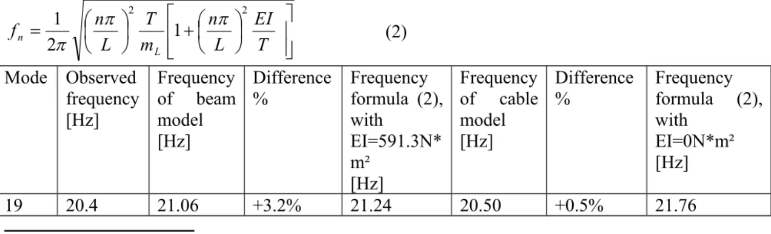
Here is a comparison between measured frequencies, frequencies computed using a cable model, frequencies computed using a beam finite element model and frequencies computed thanks to the following formula [9] (using the same tension values as in the model: 27.1kN for the beam and 29kN for the cable).
T EI L n m T L n f L n 2 2 1 2 1 (2) Mode Observed frequency [Hz] Frequency of beam model [Hz] Difference % Frequency formula (2), with EI=591.3N* m² [Hz] Frequency of cable model [Hz] Difference % Frequency formula (2), with EI=0N*m² [Hz] 19 20.4 21.06 +3.2% 21.24 20.50 +0.5% 21.76
2 IREQ : Institut de Recherche d’Hydro-Québec, www.Ireq.ca 3 fy
40 42.9 44.46 +3.6% 46.14 42.22 -1.6% 45.82
53 59.3 61.74 +4.1% 62.93 56.49 -4.7% 60.71
Table 2: Comparison between measured half wavelength and computed half wavelength (for the beam and cable models)
The comparison between the beam and cable model is performed respecting an imposed sag value. Given this hypothesis, tension in the beam model is worth 27.1kN and 29kN in the cable model. A discussion of the difference between eigen frequencies computed with the beam model and observed ones is presented further in the text.
The following tables compare measured mode shape information versus values computed by a modal analysis, with a cable and a beam model of the span.
Mode l/2 measured [m] l/2 beam model [] Difference% l/2 cable model [m] Difference % 19 3.51 3.51 0.2% 3.34 5% 40 1.71 1.71 0.1% 1.63 4.7% 53 1.27 1.27 0.5% 1.22 3.8%
Table 3: Comparison between measured half wavelength and computed half wavelength (for the beam and cable models)
Mode Position of node
1 measured [m] Position ofnode 1 beam model [] Difference% Position of node 1 cable model [m] Difference % 19 3.65 3.68 3% 3.34 8.5% 40 1.83 1.856 1.5% 1.63 11% 53 1.39 1.40 0.4% 1.22 12.4%
Table 4: Comparison between measured position of node 1 and computed position of node 1 (for the beam and cable models)
From the previous tables, one can see that the beam model with the assumption of constant bending stiffness (taken equal to the average bending stiffness deduced from measurements) leads to good results. The position of node 1 is computed with a difference of a few % (against 10% for the cable model), which means that the mode shape in the vicinity of the span is correctly computed. The difference between computed and measured position of node 1 is minimum for the 53rd vibration mode (0.4%). Also, half the wavelength is computed with a difference much inferior to 1% (against about 5% for the cable model).
TIME RESPONSE WITH A FORCED EXCITATION
On Ireq’s cable test bench, a vibration shaker was used to excite the cable. It was located at a distance of 1.68m of the span end opposed to the suspension clamp. In our finite element model, the vibration shaker is modelled by a vertical harmonic force acting at the same distance from span end, with the same amplitude as that measured during the tests.
Let us consider tests carried out on 30 September 2008 on Crow ACSR conductor tensioned at approximately 24%RTS.
The 19th eigen frequency computed by a modal analysis for the beam model is worth 21.152Hz. This means that there is a 3.6% difference between the computed value of the nineteenth frequency and the one measured in laboratory (20.4Hz). Such difference probably comes from one or several of the following reasons:
- no damping is considered for the present modal analysis; in reality, some damping is present, which will affect the values computed for eigen frequencies,
- the sag of the model has been tuned so as to coincide with the measured sag value, but with a tolerance of a few millimetres; also, the sag value was measured on a daily basis, and a small sag variation during the day due to temperature change may not be excluded; last, a small error in measurement is also possible,
- the cable is a complicated system with layers, stranding angle…modelled here with a simple beam element,
- the spatial discretization of the span has an impact on the computed mass and stiffness matrixes and hence on computed values of eigen frequencies.
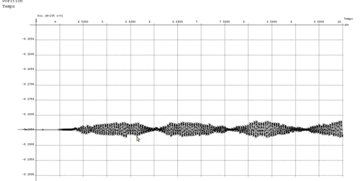
Let us now consider the dynamic response of the cable when a forced harmonic excitation, with a frequency of 21.152 Hz and the same amplitude and location as in the laboratory is introduced. The position of the third antinode (the first antinode being the one adjacent to the span end opposed to the shaker) as a function of time can be seen in figure 3. Note that the integration scheme used is Newmark with no numerical damping.
Fig. 3: Amplitude at the third antinode as a function of time (the first antinode is adjacent to the span end opposed to the shaker), when the excitation frequency of the shaker is 21.152Hz A beat is clearly visible. Its period is approximately 1.5s, which suggests that the eigen frequency of the span has been shifted of around 0.67Hz due to the introduction of the vibration shaker. Reducing by 0.67Hz the excitation frequency leads to lower amplitudes, while increasing it by 0.67Hz leads to higher antinode amplitudes of vibration.
The resonance can be visualised with a Lissajous curve, with position on one axis and excitation force on the other. At resonance, phase shift between acceleration and excitation force is 90°, which means that the Lissajous curve plotting either excitation force as a function of displacement, or excitation force as a function of acceleration is a “circle” (provided an appropriate scale is chosen for axes X and Y, else the plot will show an “unrotated” ellipse). The following figure shows a Lissajous curve for an excitation frequency of 21.85Hz.
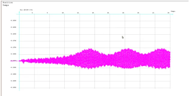
Fig. 4: Lissajous curve (position as a function of excitation) at a frequency of 21.85Hz. One can see that the phase is not constant. After some trials to stabilize the phase, it is possible to improve the situation, but not to completely get rid of beats. The best results are obtained for an excitation frequency of 22 Hz. Antinode amplitudes for a simulation at 22 Hz which does not include any damping (neither numerical nor material) reach 10mm to 15mm pk-pk. The following figure shows the position of an antinode as a function of time. The simulation time represented below is approximately 20 seconds.
Fig. 5: Amplitude at the third antinode as a function of time (antinode 1 is adjacent to the span end opposed to the shaker), when the excitation frequency is 22Hz
In reality, measured antinode amplitudes were of the order of 8mm pk-pk. Antinode amplitudes computed without any damping are therefore larger than those measured in reality, which seems logical. An interesting point is to find an explanation for the beat phenomenon.
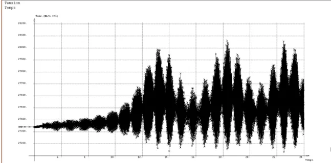
The following figure shows the evolution of tension in the beam model as a function of time. The curve suggests that the introduction of an excitation force in the model induces important tension variations. Also, the average tension once the excitation force has started is more important than the initial one. This explains why a better tuning is obtained with a higher excitation frequency.
Fig. 6: Evolution of tension in the model when the excitation frequency is 22Hz
This finding also has other consequences. The continual tension fluctuations cause a continual eigen frequency fluctuation, and even if no damping is introduced in the model, the “nodes” will be vibrating.
The Inverse Standing Wave Ration method, which is widely used to deduce conductor self damping [4] is based on the hypothesis that when no damping is present, incident and reflected wave are equal. In other words, when no damping is present, there is no motion at nodes. One may wonder how representative is the value of conductor self damping computed by this method on a span where there are tension fluctuations.
SENSITIVITY ANALYSIS
As mentioned in the introduction of the present paper, the behaviour of overhead line cables is complex to model. The present sensitivity analysis aims at studying the impact of an inaccurate value of average bending stiffness on the one hand and of excitation force in the other hand.
Experiments described in paper [1] permit to show that the relationship between conductor moment and cable rotation during loading and unloading cycles at constant speed is described by hysteretic cycles. The “shape” of these hysteretic cycles depends on conductor tension, which seems logical: interlayer friction forces depend on a friction coefficient and the pressure between layers, which directly depend on tension in the wires. When a conductor is bent, considering a cross section of the conductor, stress conditions for wires most distant from the neutral axis are very different. Since overhead cables are helicoidally wired, in a same wire, axial stress may vary along the conductor, which in turn has an impact on pressure between layers and therefore on friction forces. It is important to note that once slipping between layers has started, the moment in the conductor depends not only on conductor curvature, but also on the tension in the conductor [1].
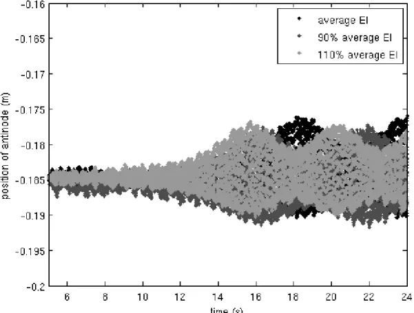
The following figure shows the impact of a 10% change in the value of average bending stiffness used in the simulations.
Fig. 7: Sensitivity of the model to the value of average bending stiffness
In the previous figure, three values of conductor bending stiffness are considered: the average one, as well as 90% and 110% of this average value. Note that the previous figure is drawn respecting a constant sag value and with a frequency adjustment performed for every case to get closer from resonance conditions. The previous figure shows that a bending stiffness change of 10% leads to an amplitude change comprised between 1 to 6%.
During the experiments performed at Ireq’s laboratory, the amplitude of the excitation force was displayed with 3 digits after the decimal commabut the measurement error on this value was probably higher than that. The following figure shows the results of a sensitivity analysis to the value of the excitation force.
. Fig. 8: Sensitivity of the model to the value of excitation force
The previous figure shows that the sensitivity to the amplitude of the excitation force is low. Considering changes of 10% in the amplitude of the excitation force, corresponding changes in maximum amplitudes computed are of the order of 5%.
Provided the value of the excitation force is of the order of a few tens of Newtons, the impact of a 1N error in the knowledge of the amplitude of the excitation force is negligible.
CONDUCTOR SELF-DAMPING
In the present paper, a first attempt to model the cable test span with beam elements is presented. The hypothesis on conductor bending stiffness has been developed in the previous paragraph. It is also interesting to discuss the way conductor self damping may be modelled.
When damping is present, in the case of a cyclic oscillation, if a force-displacement curve is plotted, its shape will be characterized by an enclosed area, also called hysteresis loop. The surface of this enclosed area represents the energy dissipation per cycle.
Under the hypothesis of a Voigt – also called Kelvin- material, which is modelled by a dashpot in parallel with a spring, when a graph of total force (spring force+dashpot force) as a function of displacement is plotted, it results in a “rotated” ellipse [7].
Plotting the bending moment in a cable as a function of bending radius, considering different loading speeds, Godinas obtained hysteresis curves [1]. Such hysteresis curves could be obtained using beam model and a Voigt-Kelvin material, where the relationship between macro stresses and macro strains could be customized. As a first trial, in the frame of the present paper, a model with a Kelvin-Voigt relationship between all stresses and corresponding strains is used. Let us explicite this hypothesis. The energy dissipated per loading cycle with a visco-elastic material and harmonic excitation is [7]:
2 d
where c is the viscous damping coefficient [N/m], omega is the angular velocity [rad/s] and X the amplitude of displacement [m]. The power dissipated is hence proportional to frequency squared (f²). As a comparison, in the experimental law given in equation (1), the power dissipated is generally expressed as a function of frequency with an exponent comprised between 4 and 6.
The following figure compares relative displacements in the vicinity of the clamp for conductor Crow tensioned at approximately 24%RTS, without any in-span equipment, for an excitation frequency of 22Hz. The test conditions are the same as those described in the paragraph “Shape of eigen modes” (fymax=80mm/s, amplitude of the excitation force equal to 26.38N), but this time, the span is modelled with beam elements, using a visco-elastic material (Kelvin-Voigt model). Three values of viscous damping parameter (alpha) are tested: 0.01, 0.001, 0.0001. When alpha is equal to 0.0001, there is still a beat phenomenon. This is why for every abscissa, two dots are plotted: one for the minimum amplitude of the beat and the other one for the maximum amplitude.
Fig. 7: Relative displacement in the vicinity of the suspension clamp, as computed with a visco-elastic material and as measured
From the previous figure, it appears that the most adequate value of parameter alpha is comprised between 0.001 and 0.0001.
With alpha taken equal to 0.0001, antinode peak-to-peak displacements comprised between 2mm and 1.3cm are obtained (a beat phenomenon is still present, these values correspond respectively to the maximum and the minimum of the beat), to be compared with the 8mm pk-pk displacements measured in reality.
It is interesting to figure an order of magnitude of the different parameters usually used to describe the damping characteristics of a system under similar conditions, using data recorded on Ireq’s cable test span. As explained in [4,7] the different parameters usually used to describe the damping characteristics of a system are:
,max4 d k E E
which is called the dimensionless damping factor for a given eigen mode (and where Ek,max is the maximum kinetic energy of the cable),
the logarithmic decrement 2 , and the loss factor
2
.
From the displacements measured at vibration nodes at the laboratory, using a correction for fluid damping proposed by Blevins [6], a loss factor value of the order of 1e-3 is obtained. The corresponding value of zeta is of the order of 0.5e-3. The corresponding value of power dissipated per unit length of the conductor is of the order of 0.01W/m for fymax=80mm/s and f=20.4Hz.
REPRODUCTION OF OBSERVED PHENOMENA WHEN IN-SPAN LINE EQUIPMENT IS INTRODUCED
During some of the tests performed with line equipment installed in-span, higher amplitudes were observed on the short portion of conductor between the line equipment and the suspension clamp, opposed to the vibration shaker side. As further explained in this paragraph, it was possible to reproduce such phenomena with the beam model computing a dynamic time response of the span, but these higher amplitudes on the short portion of span can already be observed by a modal analysis. Let us consider a vibration test made on 27 October 2008, with conductor Crow tensioned at approximately 23.5% RTS, a suspension clamp installed on the span extremity opposed to the vibration shaker, and monitoring device installed at approximately 6.2m from the suspension clamp. For an excitation frequency of 61.23Hz, amplitudes between the monitoring device and the suspension clamp were approximately 50 % higher as amplitudes between the monitoring device and the shaker. Modelling the monitoring device by a concentrated mass of 8kg, the mode shape which corresponds to the 59.44Hz eigen frequency is also characterized by higher amplitudes on the short portion of conductor between the line equipment and the suspension clamp (see figure 8).
Fig. 8: “Resonance” obtained with the beam finite element model for an eigen frequency of 59.44Hz
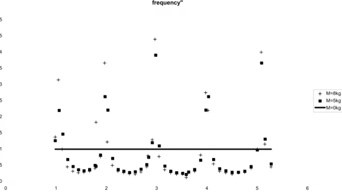
Investigating which conditions led to such higher amplitudes in the short part of the span, between the line equipment and the suspension clamps, the following graph was drawn so as to formulate the conditions which lead to this phenomenon. The graph shows the ratio between antinode amplitude on the short portion of span delimited by the line equipment device and antinode amplitude on the longest portion of span as a function of the ratio “frequency/ fundamental frequency of the short portion of span”. Three series of data are shown: the first one with the real mass value of the line equipment (8kg), the second one with a lower mass value (5kg) and the last one with no mass at all (obviously equal to 1).
Fig. 10: Ratio “antinode amplitude between suspension clamp and line equipment device/ antinode amplitude on the rest of the span” as a function of ratio “frequency/ fundamental
frequency of the portion of span between the suspension clamp and the line equipment From the previous graph, it is clear that amplitude ratios higher than 1 are met for excitation frequencies which correspond to a multiple of the fundamental frequency of the span portion between the line equipment device and the suspension clamp. Nevertheless for all other cases, the vibration amplitudes on the short portion of span are much lower than on the rest of the span. The problem needs to be further investigated, but from this information, it is possible to predict when high amplitudes will be present.
Time response
The model used to compute the time response in the previous paragraphs contains between 300 and 400 elements. With such discretization, is possible to model adequately the time response at frequencies of the order of 20 Hz, but for frequencies as high as 60Hz a mesh refinement is needed. In order not to increase the number of elements too much, it was decided to compute the time response
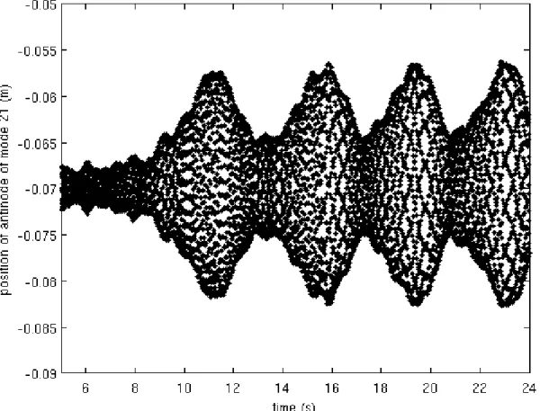
of the beam under forced excitation at a lower frequency, trying to obtain higher amplitudes on the short portion of span. The model used contains 382 elements, and a case of higher amplitudes on the short portion of span was obtained for an excitation frequency of 23.075Hz.
Fig. 11: Amplitude at an antinode located on the short portion of span when the excitation frequency is 23.075Hz
On the short portion of span, the antinodes of mode 21 vibrate with a peak-to-peak amplitude of 25mm, while on the long portion of span, antinode amplitudes of the same mode are worth 13mm peak-to-peak. This observation is equivalent to a ratio of approximately 2 between the antinode amplitudes on the short and long portion of span, which is in agreement with the values of figure 10. CONCLUSIONS
The shape of a conductor vibrating at its vibration modes in the vicinity of the span end is correctly reproduced by the beam element model.
Studying the time response of the conductor under forced excitation, it has been shown that tension fluctuations cannot be neglected in the observed phenomenon. A direct consequence is that the conductor eigen frequency continually varies, which makes it difficult to obtain a perfect resonance. For a span of this length, vibration amplitudes are worth a significant sag percentage. Part of “node” displacement is thus due to tension variation. Under such conditions, is the ISWR method still valid to estimate the cable damping properties? The ratio “amplitude of vibration/sag” on the 63m laboratory test bench is of the order of 5%, while on a real span, the same ratio is of the order of 0.2%. Therefore, smaller tension variations may be expected on real spans during Aeolian vibration events. It is
important to keep in mind the effect of tension variations when analysing a real span using self damping data coming from a “short” laboratory test span in order to avoid erroneous conclusion. Considering a concentrated mass on the conductor, modal analysis with the beam model made it possible to understand which particular conditions led to higher amplitudes on the short portion of span (between the concentrated mass and the nearest span end in our experiment). Higher amplitudes on the short portion of span occur when the excitation frequency is a multiple of the short span fundamental frequency. For all other conditions, the amplitudes of vibration on the short portion of span are lower than everywhere else. This analysis must be further completed by a study using the propagation theory. Last, it was possible to reproduce these high amplitudes on the short portion of span with a dynamic time analysis for an excitation frequency of about twenty Hz.
In the coming months, efforts will be made to improve the self damping model, bending stiffness model and further study the problem of assessing the conductor self damping on spans where tension variations may invalidate the hypotheses of ISWR.
ACKNOWLEDGEMENTS The authors warmly acknowledge
IREQ with a special thanks to Roger Paquette, Guy Brisson and Martin Gravel, Thibaut Libert and all the ampacimon team from University of Liège,
la Communauté française de Belgique. REFERENCES
[1] A. Godinas, G. Fonder, “Experimental Measurements of Bending and Damping Properties of Conductors for Overhead Transmission Lines”, Third Cable Dynamics Conf. proceedings, pp. 13-19, Trondheim (Norway), August 1999
[2] A. Cardona, 1991, “An integrated approach to mechanism analysis”, (Ph. D. thesis), Collection des Publications de la Faculté des Sciences appliquées
[3] Samtech s.a., 2008, “Samcef V13.0 User’s Manual”
[4] EPRI, 2006, Transmission Line Reference Book: Wind-Induced Conductor Motion. EPRI, Palo Alto, CA:2006.1012317
[5] K.O. Papailiou, 1997, “On the Bending Stiffness of Transmission Line Conductors”, IEEE Transactions on Power Delivery, Vol. 12, No 4, October 1997
[6] Blevins, R. D., 1977, “Flow-Induced Vibration”, New York, Van Nostrand Reinhold Co.
[7] W. T. Thomson, M. Dillon Dahlem, 1998, “Theory of Vibration with Applications”, 5th edition, Prentice Hall 1998
[8] S. Guérard, P. Van Dyke, J.L. Lilien, 2009, “Evaluation of Power Line Cable Fatigue Parameters Based on Measurements on a Laboratory Cable Test Span”, Eighth Cable Dynamics Conf. Proceedings, Paris, September 2009
[9] Newmark, N. M., 1959, “A method of computation for structural dynamics”, Proc. ASCE, J. Eng. Mech. Div. 85, pp. 67-94.