Variabilité intraspécifique de la sensibilité des macrophytes aquatiques à la contamination chimique : l'exemple du cuivre

THÈSE

En vue de l’obtention du

DOCTORAT DE L’UNIVERSITÉ DE TOULOUSE

Délivré par l'Université Toulouse 3 - Paul Sabatier

Présentée et soutenue par

Eva ROUBEAU DUMONT

Le 30 novembre 2018

Variabilité intraspécifique de la sensibilité des macrophytes

aquatiques à la contamination chimique : l'exemple du

cuivre.

Ecole doctorale : SDU2E - Sciences de l'Univers, de l'Environnement et de l'Espace

Spécialité : Ecologie fonctionnelle Unité de recherche :

ECOLAB - Laboratoire d'Ecologie Fonctionnelle et Environnement Thèse dirigée par

Arnaud ELGER et Camille LARUE Jury

Mme Gertie ARTS, Rapporteur Mme Claudia COSIO, Rapporteur

M. Nigel WILLBY, Rapporteur M. Christophe DUNAND, Examinateur

Mme Elisabeth GROSS, Examinateur M. Arnaud ELGER, Directeur de thèse Mme Camille LARUE, Co-directeur de thèse

ABSTRACT

Intraspecific variability plays a pivotal role in short and long term responses of species to environmental fluctuations. This variability, expressed through different traits of individuals, can potentially influence species sensitivity to chemical contamination. This intraspecific variability is currently not taken into account in ecotoxicological risk assessment, whereas it can mislead its results. To examine this hypothesis, the importance of intraspecific variability in the response to copper (Cu) was quantified in controlled conditions for three aquatic macrophyte species, Lemna minor, Myriophyllum spicatum and Ceratophyllum demersum. Variations among genotypes of each of these 3 species were compared to interspecific variability. Results have highlighted a significant genotypic variability, whose importance depends on the species considered. Indeed, L. minor demonstrated a low variability, contrarily to M. spicatum whose variability in growth inhibition by Cu was higher than interspecific differences. In order to specify the extent and the mechanisms of genotypic variability in M.

spicatum, other experiments involving measurements of life-history traits have been conducted

on 7 genotypes exposed to Cu. Results showed that some genotypes were up to eightfold more sensitive to Cu than others (at concentrations ranging between 0.15 and 0.5 mg/L). These differences in sensitivity were partly explained by the traits measured, but physiological or transcriptomic endpoints may explain more precisely the source of these differences in sensitivity. Finally, 3 experiments with fluctuations in nutrient concentrations, light intensity and Cu pre-exposure have demonstrated that phenotypic plasticity plays an important role in L.

minor sensitivity to Cu. Indeed, the weakening of individuals, as a result of unfavorable

environmental conditions, can lead to a two-fold increase in sensitivity to Cu. All these results demonstrated that intraspecific variability, whether it comes from genotypic variations or is linked to phenotypic plasticity, was in general lower than interspecific variability for the species and endpoints studied. However, its extent can vary depending on the species. It can therefore significantly influence aquatic macrophyte sensitivity to chemical contamination, and it would be relevant to account for it in ecotoxicological risk assessment.

Keywords: Copper, ecotoxicological risk assessment, aquatic macrophyte, intraspecific variability, genotypic variation, phenotypic plasticity

RESUME

La variabilité intraspécifique fait partie intégrante de la réponse à court et à long terme des organismes vivants aux fluctuations environnementales. Cette variabilité, exprimée au travers de différents traits des individus, peut potentiellement influencer la sensibilité des espèces à une contamination chimique. La variabilité intraspécifique n’est pas, à l’heure actuelle, prise en compte en évaluation des risques écotoxicologiques, alors même qu’elle pourrait en biaiser les résultats. Pour examiner cette hypothèse, l’importance de la variabilité intraspécifique dans la réponse au cuivre (Cu) a été quantifiée en conditions contrôlées pour trois espèces de macrophytes aquatiques, Lemna minor, Myriophyllum spicatum et Ceratophyllum demersum. Les variations entre génotypes de chacune de ces 3 espèces ont été comparées à la variabilité interspécifique. Les résultats ont mis en évidence une variabilité génotypique significative, dont l’importance dépend de l’espèce considérée. En effet, L. minor a montré une faible variabilité, au contraire de M. spicatum dont la variabilité de l’inhibition de croissance par le Cu est supérieure aux différences interspécifiques. Afin de préciser l’étendue et les mécanismes de la variabilité génotypique chez M. spicatum, d’autres expériences impliquant des mesures de traits d’histoire de vie ont été réalisées sur 7 génotypes exposés au Cu. Les résultats ont montré que certains génotypes étaient jusqu’à 8 fois plus sensibles au Cu à des concentrations allant de 0.15 à 0.5 mg/L). Ces différences de sensibilité sont en partie expliquées par les traits mesurés, mais des mesures physiologiques et/ou des approches en transcriptomique devraient pouvoir expliquer de façon plus consistante la source de ces différences de sensibilité. Enfin, 3 expériences faisant varier respectivement la teneur en nutriments, l’intensité lumineuse et la préexposition au Cu, ont démontré que la plasticité phénotypique joue un rôle majeur dans la sensibilité au Cu chez L. minor. En effet, l’affaiblissement des individus, résultant des conditions environnementales défavorables, peut conduire au doublement de la sensibilité de

L. minor au Cu. L’ensemble des résultats obtenus montre donc que la variabilité intraspécifique,

qu’elle soit d’origine génotypique ou liée à la plasticité phénotypique, demeure en règle générale inférieure à la variabilité interspécifique concernant les traits et les espèces étudiés. Cependant, son importance varie selon l’espèce considérée. Elle peut donc influer significativement sur la sensibilité des macrophytes aquatiques à la contamination chimique, et gagnerait donc à être prise en compte dans le cadre de l’évaluation des risques écotoxicologiques.

Mots clés : Cuivre, évaluation des risques écotoxicologiques, macrophyte aquatique, variabilité intraspécifique, variation génotypique, plasticité phénotypique

Acknowledgments

I will start this long list of acknowledgments by thanking my two supervisors, Arnaud Elger and Camille Larue. You have both been there to answer my questions, and gave me a direction when necessary. More particularly, I would like to thank Camille for her motivating presence during those three years (but I will come back on that later), and Arnaud for his support. Especially during the final straight line, you were present for me, you took the time to read, correct and to advise me always with patience. I can say that I really learned a lot from you, from how to structure my ideas in a paper to how to think as an ecologist, with the concepts and all. I hope I still learn from you in further collaborations. Along with that, I would like to thank Sophie Lorber, who was at the beginning my co-supervisor. Although circumstances have forced you to withdraw yourself from the board of my PhD, you always took time to see me from time to time, checking how I was doing, if everything was alright. Your kindness is something precious, and I hope you will have the chance to supervise another PhD student, to show him how enthusiast and passionate you are.

I also would like to thank the jury members, more specifically the examiners, Nigel Willby, Claudia Cosio and Gertie Arts. Their thorough review of my work, their comments and advices will help to improve my work, my experiments and deepen my scientific discussions in the future. I thank Christophe Dunand and Elisabeth Maria Gross, for their presence during my PhD defense, their questions and the discussion that followed. I have an extra-special thank for Elisabeth, who has been on the board of my PhD committee and has followed me during those three years. Thank you for your answers to the (numerous) questions I asked you about during my PhD, for your patience, and your kind and supportive presence during those two congresses.

I want to thank all of the researchers who contributed to my work during my PhD. First, Hervé Gryta, for realizing all the ISSR analysis that were necessary for the project. I appreciated your patience and your interest in this project. Elise Billoir, for her help and thorough expertise on statistical analyses, who took the time to answer my questions and helped me to progress in statistics. Benoît Pujol, for his advices during the PhD committee, his help for the plasticity experiments and his passion in his work, which was very inspiring. David Baqué, for his expertise on ICP analyses that were necessary in all of my experiments. Suzy Surble, who helped Camille and I to do experiments on the nuclear microprobe at the CEA of Saclay, but also for providing an accommodation to me and my trainee when we were running out of options. Hiram Castillo Michel, for allowing me to use the FTIR spectrometer at the ESRF at the synchrotron of Grenoble. More specifically, special thanks because I am from Grenoble and, as far as I can recall, I always wanted to see what was inside that mysterious ring.

As this goes more personal, I will continue those acknowledgments in French.

Tout d’abord, je souhaite remercier les personnes au sein du laboratoire qui ont contribué à rendre ma thèse plus simple, plus fun et plus humaine durant ces trois années. Un grand merci à Catherine Donati, une très belle personne qui rend la vie de tout le monde au labo bien plus

simple, et que j’ai pris grand plaisir à connaître. Je te remercie pour ta (très grande) patience, ta compréhension et ton humour, qui m’ont très souvent motivée et m’ont aidé à voir le bout dans les procédures administratives. De la même façon, je souhaite remercier Annick Corrège, pour son soutien et son aide précieuse pour les tâches de tous les jours qui sortaient de la réalisation d’expériences.

Je souhaite remercier tous les membres de l’équipe ECI, mais tout particulièrement Annie Perrault et Jérôme Silvestre, le combo de choc de l’équipe. Je crois que je ne peux pas dire à quel point je vous suis reconnaissante, pour tout. Vous êtes les « McGyver » du labo, et vous étiez les première personnes que j’allais voir lorsque j’avais un souci d’expérience ou une question technique. Sans vous, ma thèse n’aurait pas été la même, votre soutient en toutes circonstances et nos échanges ont été parmi les choses qui m’ont permis de persévérer. Tout simplement, merci.

Camille Larue, que je remercie encore une fois, en tant qu’amie cette fois-ci. Car c’est bien ce que tu as été dès le début de ma thèse : une amie, auprès de laquelle j’avais des discussions scientifiques sur toutes les thématiques, mais également des conversations sur tout et rien à la fois (avec pleins de questions bizarres comme je les aime). Tu es devenue mon mentor, la personne qui m’aidait à aller chercher toujours plus loin, à voir les choses autrement, avec une autre perspective. Tu es aussi celle qui m’a aidé à concilier vie sociale & vie pro, à relativiser et à respirer un bon coup quand je me sentais sous l’eau. Tu m’as aidé à me remettre en question, à évoluer en tant que scientifique, mais surtout en tant que personne. Tu es la personne à laquelle j’aimerais ressembler d’ici quelques années : passionnée, enthousiaste, l’esprit toujours curieux de tout, désireuse d’apprendre et profondément humaine. J’espère vivement continuer à travailler avec toi à l’avenir… J’ai hâte de voir jusqu’où tu vas aller : je n’ai pas oublié que tu comptes sauver la planète ;). Qui sait ce que te réserve l’avenir ?

Je souhaite particulièrement remercier Diane Espel, dont l’arrivée au labo a révolutionné la vie là-bas. Tu es une belle personne, et je peux dire que ton sourire, ton humour, ton (petit ?) accent du sud vont énormément me manquer. Il s’en sera passé des choses en 2ans et demi… En passant par les Mariposa à la province, je n’ai que de beaux souvenirs avec toi (la sortie Camargue et les waders ;)), et je sais que ça ne s’arrêtera pas là. Vive la team macrophyte ! Je souhaite également remercier Laura Lagier, Antoine Firmin et Clarisse Liné, pour leur présence au laboratoire, leur sourire et leur amitié. Restez passionnés par ce que vous faites. Je dois également remercier mes stagiaires, en particulier Maëlle Bériou, actuellement en thèse au Canada et dont le passage au labo a été très agréable, mais aussi Lucas Vigier et Céline Azéma, mes deux derniers stagiaires super motivés, jamais découragés (ou presque ;)), qui m’ont permis de finir mes dernières expériences et ma thèse sur une note particulièrement heureuse. Je vous souhaite d’aller jusqu’au bout de vos rêves, de ne jamais baisser les bras pour faire ce que vous souhaitez.

En continuant sur ma lancée, je ne pouvais pas faire autrement que de te remercier, Marion Garacci. On a vécu cette thèse ensemble, les hauts & les bas, les joies et les déprimes. Je pense qu’il ne s’est pas passé une chose que je n’aie partagée avec toi durant ces 3ans. Merci pour

tous ces moments passés. Tu as les capacités pour faire tout ce que tu veux, alors rêve haut et rêve fort, et vois où cela te mène !

Je souhaite aussi remercier mes amis des doctoriales, ces personnes géniales que j’ai rencontrées lors de ce challenge interdisciplinaire entre thésards. En particulier Paul, Nicolas et Mounir, mais aussi Quentino & Quentin, Chaimae, Julie et Cyril. Pour leur humour, ces moments de partage & de compréhension que seuls les thésards peuvent avoir lorsqu’ils sont sous pression et qu’ils pensent que le ciel leur tombe sur la tête (ou presque).

Je dois forcément remercier Céline et Marie, sans qui je ne serais pas allée aussi loin. Je vous avais promis un passage dans mes remerciements pour tout ce que vous avez fait pour moi ces dernières années, alors le voilà ! Comme nous savons toutes les trois que je pourrais écrire autant de pages que je parle (et donc, beaucoup), je vais essayer d’être brève. Céline, c’est toi qui m’a fait réaliser que je pouvais aller plus loin, que j’étais capable de beaucoup, et que les seules limites que nous avons sont celles que nous nous posons. Outre notre duo de choc à la fac, les heures passées ensemble pour toujours apprendre plus, tu as été une véritable amie depuis notre rencontre. Nous sommes très semblables dans notre désir d’apprendre, d’évoluer, de nous challenger. Qui sait où l’on sera dans 10 ans ? Marie, c’est toi qui m’as donné envie de partir à l’étranger pour découvrir autre chose, de sauter vers l’inconnu, de prendre des risques… C’est ton amitié et ton soutient inconditionnels qui me portent dans les moments forts comme dans les moments les plus bas. Sans toi, je ne serai pas celle que je suis aujourd’hui, ouverte sur le monde et les idées nouvelles. Tu es celle avec qui je partage mes espoirs et mes rêves, et qui ne rigole jamais (ou presque) de mes idées farfelues, à qui je peux montrer le meilleur comme le pire sans jamais être jugée.

Et enfin … Je souhaite remercier ma famille. Les mots me manquent pour dire à quel point je suis reconnaissante pour votre soutient durant toutes ces années, mais tout particulièrement pour ces 3 dernières. Pour toujours avoir plus confiance en moi que je n’en ai envers moi-même, pour respecter mes choix qui ne sont pas toujours les plus simples, et pour toujours, toujours croire en moi et en ce que je peux accomplir. Merci. Pour tout ça, et pour tout le reste.

CONTENTS

INTRODUCTION

(Version française résumée)

11

1. Impacts de l’homme sur l’environnement 13

2. L’environnement aquatique, réceptacle ultime de la contamination chimique 14

3. Ecotoxicologie et évaluation des risques écotoxicologiques 15

A. Prise de conscience et développement de l’écotoxicologie 15

B. Politiques environnementales 16

C. Les macrophytes, un modèle biologique aquatique pertinent 16 D. La variabilité intraspécifique en évaluation des risques écotoxicologiques 17

CHAPTER I - INTRODUCTION

19

1. Aquatic macrophytes 21

A. Definition and evolutionary history 21 B. General traits of vascular aquatic macrophytes 21

C. Habitat diversity 23

D. Ecological services 23

E. Role of macrophytes as bioindicators and biomonitors in aquatic ecosystems 24

2. Copper fate and toxicity in the environment 26

A. Generalities 26

B. Copper dissemination in the environment 27

C. Copper in living organisms 29

3. Policies and methodologies in ecotoxicological risk assessment 31

A. History of environmental regulations 31 B. Introduction to ecotoxicological risk assessment 33 C. Ecotoxicological risk assessment in Europe 34 D. Ecotoxicological risk assessment in other countries 36 E. Tiered approach in ecotoxicological risk assessment 36 F. Toxicity data used in ecotoxicological risk assessment 38 G. Species Sensitivity Distribution (SSD): a tool for ecotoxicological risk

assessment 39

H. Limits of ecotoxicological risk assessment and pitfalls of the SSD approach 40

4. Ecological importance of intraspecific variability 42

A. What is intraspecific variability? 42

B. Genetic variations 43

C. Phenotypic plasticity 45

D. Implications of intraspecific variability in species evolution and ecosystem

resilience 49

E. Intraspecific variation in risk assessment approaches 53

2

CHAPTER II - MATERIAL AND METHODS

59

1. Model species 61

A. Lemna minor 61

B. Myriophyllum spicatum 65

C. Ceratophyllum demersum 70

2. Copper exposure and experimental designs 74

A. Growth chamber parameters 74

B. Effective Cu concentrations in water samples 75 C. Intraspecific and interspecific variations 75

D. Genotypic variability 76

E. Phenotypic plasticity 77

3. Plant responses to copper 78

A. Growth related endpoints 78

B. Maximal Quantum Yield of PSII (Fv:Fm) 79 C. Cu concentrations in plant samples 81 D. Biomacromolecule analyses using FTIR spectroscopy 82 E. Genetic differentiation using Inter Simple Sequence Repeats 83

CHAPTER III - Importance of intraspecific variation on macrophyte

sensitivity to chemicals

87

1. Does intraspecific variability inflect macrophyte sensitivity to copper? 89

1. Abstract 91

2. Introduction 92

3. Materials and methods 94

A. Studied species and chemicals 94

B. Genetic differentiation of strains by ISSR 96

C. Effective Cu concentration 96

D. Growth experiments 97

E. Maximum quantum yield of photosystem II (Fv:Fm) experiments 98

F. Calculations and statistics 99

4. Results 100

A. Effective concentrations in the exposure media 100 B. Intraspecific variations in plant sensitivity to copper 100 C. Relative importance of intraspecific vs. interspecific variations 104

5. Discussion 106

A. Endpoint sensitivity 106

B. Intraspecific variation 107

C. Interspecific variation in Cu sensitivity 108

6. Conclusion 109

3

8. Supplementary data 110

CHAPTER IV - Influence of genotypic variability on Myriophyllum

spicatum exposed to chemicals

115

1. Does genotypic variability of M. spicatum affect its sensitivity to copper? 117

2. Abstract 119

3. Introduction 120

4. Material and methods 122

A. Growth and copper exposure 122

B. Distinction of genotypes 123

C. Copper concentration in water samples 123

D. Life-history traits 124

E. Biomacromolecule composition 124

F. Endpoints assessing Cu sensitivity 125

G. Statistical analyses 126

5. Results 126

A. Genetic differentiation of the seven genotypes 126 B. Differences in life-history traits among genotypes 127 C. Relationship among life-history traits 129 D. Copper impact on M. spicatum: general patterns and intraspecific

variation 130

6. Discussion 134

A. Intraspecific trait variability and trait syndromes 134 B. Variations in copper sensitivity 135 C. Implications of intraspecific variation for ecotoxicological risk assessment 137 D. Ecological implications of intraspecific variation 137

7. Conclusion 138

8. Acknowledgments 139

9. Supplementary data 140

CHAPTER V - Influence of phenotypic plasticity on macrophyte sensitivity

to chemicals

143

1. Does phenotypic plasticity inflect the sensitivity of Lemna minor to copper? 145

2. Abstract 146

3. Introduction 147

4. Material and methods 149

4

B. Endpoints 152

C. Statistical analysis 153

5. Results 154

A. Light variation 154

B. Variation in nutrient concentrations 156

C. Effect of copper pre-exposure 158

6. Discussion 160

A. Phenotypic plasticity of L. minor exposed to copper 160 B. Ecological and ecotoxicological implications 161

7. Conclusion 162

8. Acknowledgments 162

CHAPTER VI - GENERAL DISCUSSION

163

1. The importance of intraspecific variability of aquatic macrophytes in the response to

chemical contamination 165

2. Genotypic variability in the sensitivity of Myriophyllum spicatum to chemicals 167 3. Implication of phenotypic plasticity in the response of aquatic plants to chemical stress

168

4. Implications for ecotoxicological risk assessment 170

5. Limitations 171

CONCLUSION & PERSPECTIVES (english)

173

CONCLUSION & PERSPECTIVES (french)

177

5

TABLE OF FIGURES

Short introduction (Français)

Figure 1.1. Evolution de la population mondiale entre 1950 et 2100. Source: Secrétariat des Nations Unies, prévision de la population mondiale, révisions de 2017 (United Nations 2017). ... 13 Figure 2.1. Voies d’entrée de la contamination chimique dans les environnements aquatiques

(Ærtebjerg et al. 2003). ... 15 Figure 1.1. Zonation of the different vascular aquatic plants, depending on their life history

traits: emergent plants, floating-leaved plants, submerged plants, free-submerged plants and free-floating plants. ... 22

CHAPTER I

Figure 2.1. Major uses of copper: usage by region and end use sector, 2016. Graphic from the International Copper Study Group, ICSG [http://www.icsg.org/]. ROW: rest of the world. ... 26 Figure 2.2. Copper distribution in European topsoils: an assessment based on LUCAS soil

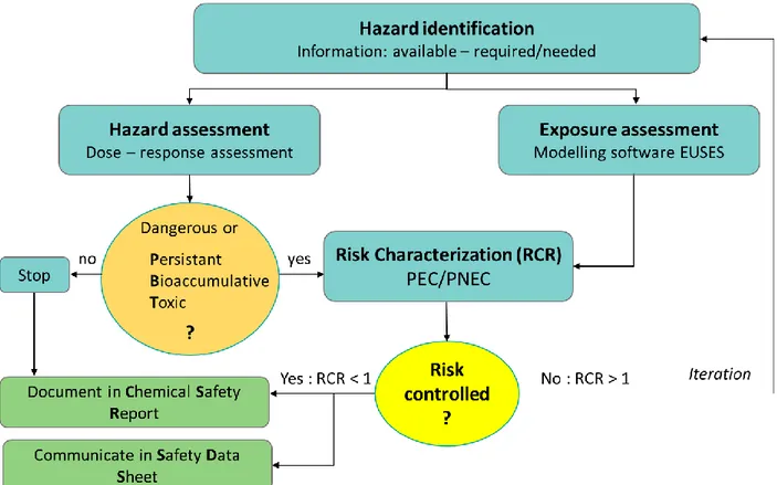
survey from 2017, and produced by Gallagher et al. 2018. The resulting map shows quite high Cu concentrations in areas typically devoted to wine production, especially in France and northern Italy. ... 28 Figure 3.1. Schematic presentation of the four steps in EU ecotoxicological risk assessment:

(1) Hazard identification, (2) hazard assessment, (3) exposure assessment and (4) risk characterization. The iteration of the process depends on the toxicity of the product and its probable environmental concentration. Adapted from the European Environment Agency (2016). ... 35 Figure 3.2. Schematic presentation of the four tiers of ecotoxicological risk assessment, with

acute (left part) and chronic (right part) effect assessment. Adapted from EFSA PPR Panel, (2013). ... 38 Figure 3.3. SSD representing the toxicity of trichlorfon in freshwater based on short‐term LC50

and EC50 values for 26 aquatic species versus the proportion of species affected. The

dashed line in black represent the HC5 (Canadian Council of Ministers of the Environment,

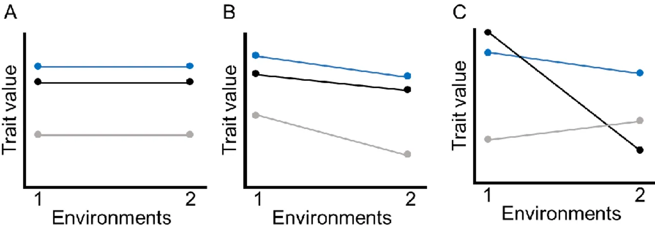
2012). ... 40 Figure 4.1. Reaction norms of a given trait of three genotypes (different color lines in each

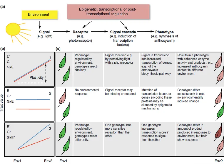
graph) under two environments, with (A) absence of phenotypic plasticity, (B) presence of phenotypic plasticity and (C) presence of phenotypic plasticity, and genotype-environment (G*E) interaction. ... 46 Figure 4.2. Phenotypic plasticity in the production of leaf anthocyanins as a defensive

6

Molecular mechanisms involved in plastic response, which translate an environmental signal (excess light in this case) into a phenotype. (b) Responses graphically presented as reaction norms. Here, the blue and red lines indicate the reaction norms of two different genotypes responding to a change from a low light environment (Env1) to a high light one (Env2). The extent of phenotypic change in response to an environmental signal is its phenotypic plasticity. Asterisks in the panels denote the significant effects of environment (E) or genotype (G), and an interaction between both (G × E). (c) Examples of the mechanisms underlying the cases depicted in panels 1–3 are given separately for each point in the signal pathway. The leaves on the left and right represent the phenotypes in Env1 and Env2, respectively. Figure from Nicotra et al., 2010. ... 47 Figure 4.3. Impact of selection and plasticity on genetic diversity, according to the cost of

plasticity. Genetic diversity is represented by different forms, and different phenotypes are represented by different colors. The population size is kept constant. (a) Without plasticity, showing a strong decline of genetic diversity, (b) with equal plasticity among genotypes and a very strong cost of plasticity resulting in a strong decline of genetic diversity; (c) with equal plasticity among genotypes and a medium cost of plasticity for the circles and strong cost for the rectangles resulting in a low decline of genetic diversity, and (d) with equal plasticity among genotypes and no cost of plasticity, resulting in the maintenance of genetic diversity. Figure from Grenier et al. 2016. ... 51 Figure 4.4. Graphical scheme representing the potential impact of intraspecific variation in

chemical sensitivity, with (a) genotypic variability among four genotypes of aquatic plants and (b) phenotypic plasticity in the chemical sensitivity of one genotype across four environmental sets. Genotypic variability takes time, as it occur through several generations, whereas phenotypic plasticity occur during an individual lifespan. Phenotypic plasticity is a costlier process, as it require sensors for environmental cues, and constant adjustments, compared to a fixed trait which will not vary across environmental ranges. ... 54 Figure 5.1. Graphical scheme of the questions addressed during my PhD project. Importance

of intraspecific compared with interspecific variations in three macrophytes species exposed to copper (Cu), with several genotypes per species (A). Underlying mechanisms of intraspecific variation with (B) importance of genotypic variability in the sensitivity of seven genotypes of Myriophyllum spicatum exposed to Cu and (C) importance of phenotypic plasticity in the sensitivity of Lemna minor exposed to Cu under favorable and unfavorable environments (Envi.). ... 56

CHAPTER II

Figure 1.1. (A) Lemna minor in an axenic culture inside an Erlenmeyer flask, (B) close-up picture of L. minor controls during Cu exposure. Both pictures were taken in a growth chamber. ... 61 Figure 1.2. Distribution map of Lemna minor across the globe. Red dots are the countries/states

where the species has been reported (CABI, Centre for Agriculture and Biosciences International, 2011, [www.cabi.org/isc/]). ... 63

7

Figure 1.3. (A) Geographic origin of the different clonal strains of L. minor used for experiments and (B) GPS location of the harvesting sites. ... 64 Figure 1.4. (A) Picture of stock culture of Myriophyllum spicatum in a 220 L outdoor tank, (B,

C) pictures of M. spicatum in another stock culture in the growth chamber in an 80 L aquarium. ... 66 Figure 1.5. Distribution map of Myriophyllum spicatum across the globe. Red dots are the

countries/states where the species has been reported (CABI, Centre for Agriculture and Biosciences International, 2011, [www.cabi.org/isc/]). ... 67 Figure 1.6. (A) Geographic origin of the different clonal strains of Myriophyllum spicatum used

for experiments and (B) GPS coordinates of the harvesting sites. ... 68 Figure 1.7. Growth media for Myriophyllum spicatum tested with sediments mixed with

Osmocote® over 10 days. S&B: Smart and Barko media pH6.5, Andrew media pH6.5 and Steinberg media pH6.5. RER stands for Relative Elongation Rate in cm.cm-1_.d-1_{, and RGR}

for Relative Growth Rate in mg.mg-1.d-1. ... 69 Figure 1.8. (A) Stock culture of Ceratophyllum demersum in an 80 L aquarium in a growth

chamber with M. spicatum, (B) close-up picture of C. demersum shoots. ... 71 Figure 1.9. Distribution map of Ceratophyllum demersum across the world. Red dots indicate

the countries/states where the species has been reported (CABI, Centre for Agriculture and Biosciences International, 2011, [www.cabi.org/isc/]). ... 72 Figure 1.10. (A) Geographic origin of the different clonal strains of Ceratophyllum demersum

and (B) GPS coordinates of the harvesting sites. ... 73 Figure 1.11. Relative Elongation Rate (RER) based on length in cm.cm-1.d-1, and Relative

Growth Rate (RGR) based on fresh in mg.mg-1.d-1 of Ceratophyllum demersum growing in different media during 7 days. Stb: Steinberg, Hoag.: Hoagland. ... 74 Figure 2.1. Exposure conditions to ionic Cu for the three species (A) Lemna minor in Steinberg

medium, (B) Ceratophyllum demersum in half strength Steinberg, (C) Myriophyllum

spicatum in Smart & Barko medium with sediment. ... 76

Figure 2.2. Experimental design to highlight the phenotypic plasticity in the response of Lemna

minor exposed to Cu, with an acclimatization phase (14 days) and exposure phase (7 days).

... 77 Figure 3.1. A simplified description of the steps occurring in PSII explaining the main

parameters in fluorescence analysis. (A) A schematic figure showing electron transport within the PSII reaction centre complex. Light energy is absorbed by chlorophyll within the light-harvesting complex, and can be dissipated either via photochemistry, by heat (non-photochemical quenching), or through fluorescence emission. The competition between these processes allows us to resolve the efficiency of PSII. LHC= Light Harvesting Complex, CP = Chlorophyll-proteins, Pheo = Pheophytin, QA and QB =

Quinones A and B, PQ = Plastoquinone, OEC = Oxygen-Evolving Complex. (B) Fluorescence trace made on dark-adapted leaf material, showing the formation of Fo and

Fm. The measuring beam excites chlorophyll, but its energy is not of a sufficient intensity

8

level of fluorescence. At this state, the reaction centres are said to be open. Then a saturating pulse of light will result in the formation of the Fm, which is the formation of the maximum possible level of fluorescence, as this pulse closes the reaction centres. (Adapted from Murchie & Lawson, 2013). ... 80 Figure 3.2. Sample analysis using ICP-AES method with the different steps, from the

nebulization of the sample to its ionization in the plasma flame, and the separation of the wavelength spectrum and its detection by the detector, ending with concentration determination by the computer. ... 82 Figure 3.3. Genotypic differentiation with PCR amplification using an ISSR primer on three

genotypes of M. spicatum. First, DNA is extracted from fresh plant material, and amplified through a PCR step using ISSR primers. Finally, amplified fragments were separated through electrophoresis. ... 84

CHAPTER III

Figure 1.1. Summary of the experimental design to assess the influence of intraspecific variability, more specifically genotypic variation, in three aquatic macrophyte species sensitivity to copper contamination. At least three genotypes of Lemna minor,

Ceratophyllum demersum and Myriophyllum spicatum were exposed to Cu. ... 90

Figure 2.1. Sensitivity to chemicals for five hypothetic species determined using individuals from a single population per species (in black). In this kind of approach, the real variability of the species response to contamination is ignored, and interspecific differences which are highlighted here may be spurious and result from a “sampling effect” (i.e. these differences may be related more to the sensitivities of the populations sampled than to intrinsic characteristics of the species). ... 94 Figure 4.1. Concentration-response curves for three genotypes of L. minor exposed to copper,

with relative growth rates (RGR) based on fresh weight (A) and frond number (B) after 7 days of exposure, and (C) Fv:Fm after 96h. Curves were fitted with non-linear log-logistic

models with 4 parameters (A and B) and 3 parameters (C). ... 101 Figure 4.2. Concentration-response curves for four genotypes of M. spicatum exposed to

copper, relative growth rates (RGR) based on fresh weight (A) and shoot length (B) after 12 days of exposure. Curves were fitted with non-linear log-logistic models with 3 parameters. ... 103 Figure 4.3. Concentration-response curves for two to three genotypes of C. demersum exposed

to copper, with relative growth rates (RGR) based on fresh weight (A) and shoot length (B) after 14 days of exposure, and Fv:Fm (C) after 96h. Curves were fitted with non-linear

log-logistic models with 4 parameters for growth related endpoints (A, B) and exponential decay models with 2 parameters for Fv:Fm (C). ... 104

Figure 4.4. EC50 values for Relative Growth Rates based on fresh mass of three species, L.

minor, M. spicatum and C. demersum exposed to copper. From three to four genotypes of

each species were exposed during 7 days (L. minor), 12 days (M. spicatum) or 14 days (C. demersum) to concentrations from 0 to 1.25 mg/L, 0 to 2 mg/L and 0 to 0.5 mg/L Cu,

9

respectively. Same letters within a given species indicate genotypes whose EC50 values do

not differ significantly. ... 106

CHAPTER IV

Figure 1.1. Geographic origin of the 7 genotypes of M. spicatum used to assess the influence of genotypic variability in chemical sensitivity. ... 118 Figure 5.1. Life-history traits measured on 7 genotypes of Myriophyllum spicatum in absence

of copper contamination. RERall, Relative elongation rate based on total shoots length (A), Main shoot elongation (C), whorl number (D), lateral shoot development (E), relative growth rate based on fresh mass (F), dry matter content (G) and root number (H) were measured. The legend with color code is displayed in (B). ... 128 Figure 5.2. Principal component analysis conducted on wavelength numbers from FTIR

analysis, performed on five genotypes of Myriophyllum spicatum. ... 129 Figure 5.3. Principal Component Analysis (PCA) performed on 7 life-history traits for 7

genotypes of Myriophyllum spicatum. Relationship between Relative Growth Rate (RGR), Relative Elongation Rate based on total shoot length (RERall); RER based on main shoot elongation (RERmain), whorl number per cm (whorls_cm), Dry Matter Content (DMC), root number (Roots) as well as lateral shoot number (LS) is assessed. Color gradient represents the goodness of representation of each variable in the factorial plan defined by axes 1 and 2. ... 130 Figure 5.4: Copper sensitivity of 7 genotypes of Myriophyllum spicatum, assessed through the

inhibition of their Relative Growth Rates (RGR) (A) and Relative Elongation Rates based on total shoots elongation (RERall) (B) during a 10-day exposure. ANOVA P-values for genotype effects are provided; genotypes with same letters for a given combination endpoint x Cu concentration are not significantly different in terms of copper sensitivity (HSD Tukey test). ... 131 Figure 5.5: Linear discriminant analysis on 7 genotypes of Myriophyllum spicatum exposed to

Cu during 10 days. The left panel displays the canonical weights of the different variables, with the number of whorls/cm, the number of lateral shoots (LS), Cu plant concentration, dry matter content (DMC), RGR (Relative Growth Rate based on fresh mass), RERall (Relative Elongation Rate, based on total shoots length) and RERmain (RER based on main shoot elongation). The percentages correspond to the inertia of each axis. The right panel displays the scores of the experimental units. These were grouped with ellipses and labelled after the combination genotype x Cu concentration. ... 133

CHAPTER V

Figure 4.1. The crossed experimental design used in our study, with an acclimatization and a copper exposure phase. One environmental factor (light intensity, nutrient level or copper pre-exposure) varied per experiment, with ‘favorable’ and ‘unfavorable’ conditions for plant growth. For example, light intensity was either the one routinely used on the stock

10

cultures, and considered as ‘favorable’ (L+), or lowered using a shading mesh, and considered as ‘unfavorable’ (L-) for plant growth. The various combinations of conditions during acclimatization and Cu exposure allowed to avoid any confounding effect of environmental conditions prior to the experiment, and to distinguish between the effects of average environmental conditions and of temporal change regime. ... 150 Figure 5.1. (a) Maximum quantum yield (Fv:Fm) of L. minor under favorable” (L+) and

“unfavorable” (L-) light conditions during the phase of acclimatization (first letter in the legend) and the phase of Cu exposure (second letter in the legend). (b) Relative growth rate (RGR) based on biomass production under “favorable” (- / L+) and “unfavorable” (- / L-) light conditions during Cu exposure at 0, 0.05 and 0.25 mg/L. Only steady conditions are shown in figure 1b, as no significant effect of acclimatization was found. Significant differences among treatments and Cu concentrations are labelled with different letters from a to d, error bars correspond to standard errors. ... 155 Figure 5.2. (a) Maximum quantum yield (Fv:Fm) and (b) relative growth rate (RGR) of L. minor

under “favorable” (N+) and “unfavorable” (N-) nutrient concentrations (KNO3 and

KH2PO4) during the phase of acclimatization (first letter in the legend) and the phase of

Cu exposure (second letter in the legend), at 0, 0.1 and 0.25 mg/L. Significant differences among treatments and Cu concentrations are labelled with different letters from a to h, error bars correspond to standard errors. ... 158 Figure 5.3. (a) Maximum quantum yield (Fv:Fm), and (b) relative growth rate (RGR) of L.

minor pre-exposed to 0.05 mg/L Cu or not pre-exposed before Cu exposure at 0, 0.015 and

0.2 mg/L. Significant differences among treatments and concentrations are labelled with different letters from a to d, error bars correspond to standard errors... 159

11

INTRODUCTION

(Version française résumée)

13

1. Impacts de l’homme sur l’environnement

Durant les deux derniers siècles, la révolution industrielle a mené à une forte augmentation de la population humaine (Figure 1.1). Pour répondre à ses besoins toujours croissants, des changements, notamment dans les pratiques agricoles, ont été mis en place, et ont mené à la révolution verte. Ainsi, ces cinquante dernières années, la population a plus que doublé, et la production céréalière a triplé, avec seulement 30 % d’augmentation de terres cultivées (Pingali 2012). La croissance de la population humaine, ainsi que la modification des modes de vie, ont mené à l’augmentation des besoins pour les ressources, l’énergie, la nourriture, le logement, les terres cultivables. Réponde à ces besoins demeure un challenge à l’heure actuelle (Goulding et al. 2008; Mozner 2013; García-Mier et al. 2013). De plus, cela a mené à l’augmentation des déchets sous-produits. Jusqu’à maintenant, la croissance humaine a été exponentielle, et son impact sur les écosystèmes a suivi.

Figure 1.1. Evolution de la population mondiale entre 1950 et 2100. Source: Secrétariat des Nations Unies, prévision de la population mondiale, révisions de 2017 (United Nations 2017).

Les activités humaines constituent une menace majeure pour la biodiversité de la planète, ainsi que pour la santé des écosystèmes (Tilman and Lehman 1987; Dubois et al. 2018; Dodds et al. 2013). Entre autre, ces effets nocifs sur l’environnement sont liés à un changement d’utilisation des terres (urbanisation, industrie minière), qui va perturber et morceler les écosystèmes présents. Ces activités produisent également une multitude de polluants tels que

14

des hydrocarbures aromatiques polycycliques (HAP), des éléments traces métalliques (ETM), des nanoparticules, des hormones ou encore des microplastiques, avec de nombreuses voies d’entrée dans les écosystèmes.

2. L’environnement aquatique, réceptacle ultime de la contamination

chimique

Les eaux douces occupent seulement 0.8 % de la surface planétaire, mais sont l’habitat d’environ 6 % des espèces existantes (Woodward et al. 2010).

En raison de différents processus, tels que l’érosion des sols, la volatilisation atmosphérique et la redéposition des polluants en suspension, les écosystèmes aquatiques sont le réceptacle final de la contamination chimique (Figure 2.1, Ærtebjerg et al. 2003; Woodward et al. 2010). Selon Dodds et al. (2013), les impacts anthropiques sur les écosystèmes d’eau douce sont globaux. Ils peuvent entre autres altérer le flux d’écoulement, causer des invasions biologiques, des altérations thermiques, causer des extinctions biologiques ou encore des contaminations chimiques et ainsi menacer l’équilibre fragile de ces écosystèmes, et donc à plus ou moins long terme mettre en péril les services écosystémiques rendus. Les services écosystémiques sont définis comme les bénéfices que les humains retirent des écosystèmes, tels que la production d’oxygène, de biomasse (bois, nourriture pour l’homme ou pour les animaux d’élevage), ou encore l’activité des pollinisateurs pour les cultures (Seppelt et al. 2011). Enfin, les humains utilisent également une portion substantielle de cette ressource en eau douce, que ce soit pour leur survie ou leurs activités domestiques et industrielles (Dodds et al. 2013).

15

Figure 2.1. Voies d’entrée de la contamination chimique dans les environnements aquatiques (Ærtebjerg et al. 2003).

3. Ecotoxicologie et évaluation des risques écotoxicologiques

A. Prise de conscience et développement de l’écotoxicologie

Certains événements ont contribué à la prise de conscience globale de l’effet néfaste que nos activités pouvaient avoir sur les écosystèmes. Entre autres, l'explosion de la première bombe atomique dans le désert du Nouveau-Mexique en 1945, qui marque l’aboutissement du projet Manhattan et la contamination des écosystèmes par des composés radioactifs. Un autre exemple fut la guerre du Vietnam, qualifiée de guerre écologique car elle détruisit durablement des écosystèmes au moyen d'herbicides de synthèse (Neilands 1970; Prăvălie 2014). Certaines publications ont également eu un retentissement très important, tels que le livre ‘Silent Spring’ de Rachel Carson, paru en 1962, qui a démontré que l'arme atomique n'était pas la seule à menacer de détruire la vie, et que les pesticides pouvaient à long terme conduire à des résultats similaires. Ce livre a notamment mené à la création des premières lois environnementales aux Etats-Unis et à la formation de l’agence de protection environnementale (US-EPA). En réponse

16

à cette prise de conscience croissante, un nouveau champ disciplinaire s’est développé dans les années 1970, l’écotoxicologie, qui vise à étudier la toxicité des activités humaines sur l’environnement (Truhaut 1977).

B. Politiques environnementales

Au niveau politique, afin de limiter l’impact de l’homme sur l’environnement, plusieurs mesures ont été mises en place, à la fois pour déterminer la toxicité de molécules manufacturées par l’homme, et pour évaluer et diminuer la pollution potentielle émise par certaines pratiques agricoles et/ou industrielles. Notamment, la Directive Cadre sur l’Eau européenne a été implémentée en octobre 2000, afin de limiter l’impact des activités humaines sur les écosystèmes aquatiques, et augmenter leur qualité (European Commission 2000). Par ailleurs, le règlement REACH (Enregistrement, Evaluation, Autorisation, Restrictions des Substances Chimiques règlement n°1907/2006) a été mis en place en 2007 afin d’évaluer la toxicité des produits chimiques présents sur le marché, ou nouvellement créés. Pour ce faire, des outils spécifiques ont donc été développés faisant l’objet de protocoles standardisés (pour plus de détails: Chapitre 1.3) se focalisant généralement sur des unités taxonomiques et/ou niveaux trophiques différents. L’évaluation des risques écotoxicologiques permet ainsi une approche intégrative, notamment au travers de tests en laboratoire sur des espèces modèles, pour déterminer la toxicité potentielle sur un écosystème donné des produits chimiques présent sur le marché.

C. Les macrophytes, un modèle biologique aquatique pertinent

De par leur place dans les écosystèmes aquatiques en tant que producteurs primaires, leurs implications dans les cycles biogéochimiques ainsi que leur sensibilité aux paramètres environnementaux, les macrophytes sont des organismes très pertinents pour évaluer l’impact potentiel de molécules sur les écosystèmes. En effet, ces organismes chlorophylliens visibles à l’œil nu sont pour la plupart sessiles, et sont de ce fait, utilisés en tant que bioindicateurs de l’état de santé des écosystèmes aquatiques. En d’autres termes, ils attestent de la qualité physico-chimique d’un écosystème de par leur présence, leur diversité ainsi que leur réponse métabolique. Ils sont également utilisés en biosurveillance car l’analyse de leurs tissus reflète souvent le degré de contamination de leur environnement (Haury et al., 2001; Ferrat, Pergent-Martini et Roméo, 2003). Si leur capacité à accumuler les polluants est un atout pour utiliser

17

ces organismes en tant que sentinelles au sein des écosystèmes, c’est également la raison pour laquelle les macrophytes sont parmi les premiers organismes impactés par les contaminations d’origine anthropique.

Ces organismes sont faciles à manipuler en laboratoire, et sont aujourd’hui incontournables dans les tests de toxicité en laboratoire. De ce fait plusieurs protocoles standardisés ont été mis au point sur les macrophytes par l’Organisation de Coopération et de Développement Economique, ou OCDE (OECD 2006, 2014a, 2014b).

D. La variabilité intraspécifique en évaluation des risques écotoxicologiques

L’impact des polluants organiques comme des ETM sur les macrophytes aquatiques a été démontré dans diverses publications (Pflugmacher et al. 1997; Samecka-Cymerman and Kempers 2004; Knauert et al. 2010; Ladislas et al. 2012). Afin d’améliorer continuellement les démarches d’évaluation des risques écotoxicologiques, leur pertinence et leur transposition in

situ, de nombreuses études essaient de rendre compte des facteurs qui ne sont pas encore pris

en compte dans ces approches (Belanger et al. 2017; Maltby et al. 2005; Forbes and Calow 2002; Pathiratne and Kroon 2016). C’est dans ce contexte que s’inscrit ce travail de thèse, qui vise à étudier l’importance de la variabilité intraspécifique de la réponse des macrophytes aquatiques face à une contamination chimique.

La variabilité intraspécifique peut être définie comme la variabilité observable entre des individus d’une même espèce. Cette variabilité est le fruit de différences génétiques entre ces individus, et de l’influence de l’environnement sur l’expression de leur patrimoine génétique. Elle est considérée comme une étape clé dans l’évolution des espèces et leur adaptation à un nouvel environnement, et les différents mécanismes impliqués sont expliqués plus en détails dans le chapitre I.4. Cette variabilité intraspécifique n’est pas prise en compte en évaluation des risques écotoxicologiques à l’heure actuelle, et elle peut potentiellement impacter de façon significative les résultats des tests en laboratoire (Chapitre I.3). En effet, beaucoup d’études font part de l’influence des facteurs environnementaux, tels que le pH ou la teneur en nutriments, sur la morphologie et la physiologie des plantes aquatiques (Puijalon et al. 2008; Vasseur and Aarssen 1992; Gratani 2014). D’autres études font état de l’importance de la diversité génétique au sein des macrophytes aquatiques, et des différences morphologiques et physiologiques entre populations qui peuvent en résulter (Eckert et al. 2008; Pollux et al. 2007; Othman et al. 2007). Cependant, à l’heure actuelle, très peu d’études ont cherché à déterminer

18

l’importance de la variabilité intraspécifique dans la réponse des plantes aquatiques aux contaminations chimiques. Cette question est pourtant très pertinente, si l’on considère l’importance de la pollution des écosystèmes par les activités humaines.

Ce projet de thèse a pour but de pallier ce manque de connaissances, et de déterminer l’impact que la variabilité intraspécifique pourrait avoir sur les procédures d’évaluation des risques écotoxicologiques telles que nous les connaissons.

Dans cette optique, nous avons cherché à déterminer l’importance de cette variabilité intraspécifique chez des plantes aquatiques exposées à un élément trace métallique, le cuivre.

Cette thèse s’articule autour de trois questions principales:

1) Quelle est l’étendue de la variabilité intraspécifique dans la réponse des plantes aquatiques à la contamination chimique ? J’ai cherché à répondre à cette question pour trois espèces dans le chapitre III.

2) Cette variabilité intraspécifique chez les plantes aquatiques est-elle expliquée par leur variabilité génotypique ? C’est ce que j’analyse dans le chapitre IV, en me focalisant sur une espèce de plante aquatique, le myriophylle en épis (Myriophyllum spicatum). 3) La plasticité phénotypique peut-elle moduler la réponse des plantes aquatiques aux

contaminations chimiques ? Les résultats que j’ai obtenus pour répondre à cette question, concernant une autre espèce, la lentille d’eau (Lemna minor), sont présentés dans le chapitre V.

19

CHAPTER I

INTRODUCTION

21

1. Aquatic macrophytes

A. Definition and evolutionary history

Aquatic macrophytes refer to large photosynthetic organisms visible to the naked eye, and adapted to partial or total life in aquatic habitats. They are represented in several plant clades, the main ones being macroalgae (Chlorophyta and Charophyta, or green algae, Xanthophyta, or yellow-green algae, Rhodophyta, or red algae, Cyanobacteria, or blue-green algae, and Phaeophyta, or brown algae), mosses (Bryophyta), ferns (Pteridophyta) and seed-bearing plants (Spermatophyta) (Haury et al. 2001; Chambers et al. 2008). Vascular macrophytes are found among ferns and seed-bearing plants.

In the early Paleozoic (541 to 251 million years ago), ancestral marine plants colonized land, giving rise to the evolution of vascular plants (Chambers et al. 2008). As angiosperms diversified and thrived in terrestrial habitats, some species came back to aquatic environments (freshwater and marine), and became aquatic. The transition back to an aquatic life has been achieved by only 3 % of the approximately 350,000 angiosperm species (Cook 1999). According to the same study, probably 252 events of independent colonization have occurred, with at least seven reversion events in ferns, and 204-245 reversion events in angiosperms.

B. General traits of vascular aquatic macrophytes

Reproductive traits and other life-history traits of aquatic angiosperms are tightly associated with their growth form (e.g. root disappearance, free-floating), as they represent different degrees of aquatic life adaptation, and are convergent among aquatic angiosperms (Thomaz et al. 2008). Angiosperms is the main group representing vascular aquatic macrophytes. They can be divided in five main life forms (Figure 1.1):

- Emergent (also known as helophyte), with plants being rooted in the sediments with above parts extending into the air, such as Typha species,

- Floating-leaved, with plants rooted in the sediments with leaves floating at the water surface, such as Nymphaea species,

- Rooted submerged, with plants that are rooted into the sediments and are completely submerged, such as Myriophyllum species,

- Free-submerged, with plants non rooted to sediments, and floating freely in the water column, such as Ceratophyllum species,

22

- Free-floating, with plants floating at the water surface without being rooted to the sediments, such as Lemna species.

Figure 1.1. Zonation of the different vascular aquatic plants, depending on their life history traits: emergent plants, floating-leaved plants, submerged plants, free-submerged plants and free-floating plants.

As a consequence of this return to aquatic life, many physiological and morphological adaptations occurred in aquatic angiosperms, in order to cope with limited CO2 (e.g. use of

bicarbonates) and reduced light and oxygen availability (Chambers et al. 2008). For instance, they have large leaf surface, often highly dissected, to increase surface area (e.g. Ceratophyllum

demersum, Myriophyllum spicatum) in order to enhance light, carbon and nutrient uptake

through an increased surface contact with the environment (Bornette and Puijalon 2009). They have a thin cuticle, and also show a high concentration of chloroplasts near the leaf surface to cope with the decreased light availability in water. They are usually poorly lignified, as water preserves plants from gravitational stress, and they are characterized by the presence of aerenchyma, a plant tissue which forms spaces or air channels in the leaves, stems and roots, and increases oxygen flux from shoots to roots. Macrophytes growing in shallow water can overcome aqueous inorganic carbon limitations for photosynthesis through the absorption of atmospheric CO2 with aerial or floating leaves.

23

Their dispersal partly relies on water drift, thus on seed buoyancy and on plant ability to break themselves up and regrow from broken fragments, and partly on anemochory and zoochory (e.g. by birds or fish). Some species can reproduce under water, relying on underwater transport of pollen, such as Ceratophyllum demersum.

Some traits found in submerged species, such as aerial pollination, aquatic pollination and presence of stomata, are interpreted only under an evolutionary perspective.

C. Habitat diversity

Aquatic macrophytes colonize a wide variety of aquatic habitats, from tiny temporary ponds to thermal springs (e.g. Najas tequefolia) passing by waterfalls (e.g. Podostemaceae family). They are also found in rivers, lakes, lagoons and reservoirs (Thomaz et al. 2008). According to Chambers et al. (2008), the diversity of vascular macrophytes is the highest in the Neotropics (984 species), intermediate in the Orient, Nearctic and Afrotropics (664, 644 and 614 species, respectively), lower in the Palearctic and Australasia (497 and 439 species, respectively), and even lower in the Pacific region and Oceanic islands (108 species). Only very few species have been found in the Antarctica, all confined to sub-Antarctic freshwater habitats.

Free-floating and tall species with floating leaves, or forming a canopy just below the water surface, are often the most competitive species for light resource, and dominate when sufficient nutrients are available in the water column, while rooted species are dominant in lotic ecosystems (Bornette and Puijalon, 2009).

D. Ecological services

Aquatic macrophytes are involved in the structure and functioning of aquatic ecosystems. They influence nutrient cycles through the transfer of chemical elements from sediments to water, by both active and passive processes, both during their growth phase and during their senescence and decomposition (Magela et al. 2010). Nutrients (phosphorus and nitrogen) and dissolved organic carbon released by aquatic plants are quickly used by micro-algae and bacteria which are free-living or attached to macrophyte surfaces (Sand-Jensen and Borum 1991). They also impact nutrient cycling through the retention of solids (detritus) and nutrients, by their submerged roots and leaves through protection against wave actions (Madsen et al. 2001). Thus, they protect sediments and riverine soils from erosion, and can inflect water

24

flow if they form dense canopies. They also influence underwater light availability, hence they interfere with photosynthesis of other organisms.

Aquatic macrophytes have been characterized as an important food resource for aquatic organisms, both through dead organic matter for detritivorous organisms, and for living organisms through grazing (Magela et al. 2010). The influence of macrophyte species on populations and communities has been widely studied for a variety of organisms. They foster species diversity, as they are substrate for several species of algae and bacteria and can provide shelter for periphyton (Van Donk and Van de Bund 2002), micro- and macroinvertebrates (Schramm and Jirka 1989; Ferreiro et al. 2010; Kouamé et al. 2011), but also interact with fish species (Theel et al. 2008; Schultz and Dibble 2012) and waterbirds (Klaassen and Nolet 2007; Guadagnin et al. 2009; Laguna et al. 2016). To draw a general picture, Scheffer (2004) illustrated the role of aquatic macrophytes as a luxuriant forest full of biodiversity.

Last but not least, some macrophyte species (e.g. rice) are widely cultivated for human consumption and represent a major food source for many populations.

However, several of the worst invasive weeds are aquatic macrophytes, e.g., Myriophyllum

spicatum in North America, Eichhornia crassipes in China, Hydrilla verticillata in the US, Ludwigia grandiflora in Southern Europe (Olden and Tamayo, 2014; Wang et al., 2016; Zhu et al., 2017).

E. Role of macrophytes as bioindicators and biomonitors in aquatic ecosystems

A bioindicator is defined as an organism (or a part of an organism) or a community of organisms, that provides qualitative information on the environment, whereas a biomonitor is an organism or a community of organisms that provides quantitative information of environmental status (Markert et a. 2003). Some species are also considered as ‘sentinel’, as these species accumulate and concentrate pollutants from their surroundings and the analysis of their tissues provides an estimate of the environmentally available concentrations of pollutants (Gerhardt 2011).

The role of macrophytes as bioindicator and for biomonitoring has been extensively studied over the years. As primary producers, and due both to their involvement in aquatic ecosystem functioning and their sensitivity to environmental modifications, they are an ideal tool to assess ecosystem health. For instance, Pereira et al. (2012) have demonstrated that

25

macrophyte communities were relevant bioindicators of limnological conditions of lakes in southern Brazil, as species richness and growth-forms varied depending on nutrients, pH and dissolved oxygen. Furthermore, it was often demonstrated that submerged macrophyte community and diversity respond to changes in the nutrient concentrations of their environment (Kohler and Schneider 2003; Lukács et al. 2009).

To go further, several methodologies based on macrophyte composition, diversity and abundance, have been developed to assess the ecological status of freshwater ecosystems, as tools for the Water Framework Directive (see chapter I.3). For instance, the LEAFPACS method uses macrophyte composition to define ecological quality of rivers and lakes (Willby, Pitt, and Phillips 2012; Penning et al. 2008). Other methods exist, such as the Trophic Index of Macrophytes (TIM) and the Macrophyte Biological Index for Rivers (IBMR) in running waters, or the Macrophyte Index (MI) and the Ecological State Macrophyte Index (ESMI) in lakes (Kohler and Schneider 2003; Fabris et al. 2009; J. Haury et al. 2006; Ciecierska and Kolada 2014).

Many studies focused on the assessment of chemical pollution by macrophytes. For instance, Ladislas et al. (2012) have demonstrated that aquatic plants were relevant to assess metal pollution in ecosystems, as plant concentration indicated cumulative effects of environmental pollution from water and sediment. Khellaf and Zerdaoui (2010) have shown that Lemna minor was highly relevant in biomonitoring program of copper contamination. Ferrat et al., (2003) have suggested that seagrasses showed an early response to environmental pollution, and are thus good bioindicators. Likewise, several species of macrophytes were successfully used in Russia to evaluate trace element contamination of water bodies (Kurilenko and Osmolovskaya 2006). Aquatic macrophytes are therefore highly relevant to assess the toxicity of given molecules, or the impact of agricultural practices through runoffs of crop soils, as well as wastewater treatment quality, among others.

The ability of some species to take up trace elements, as well as to thrive in highly eutrophic waters (i.e. rich in ammonia and phosphorus) has led to the development of depollution practices, such as phytoremediation to remove pollutants from sediments and water, or for wastewater treatment (Nirmal Kumar et al. 2008; Dosnon-Olette et al. 2011; Nair and Kani, 2016; Newete and Byrne, 2016). The use of macrophytes in phytoremediation of copper has been extensively studied as this metal is broadly found in aquatic ecosystems due to multiple uses, and because its excess is known to cause damages to aquatic organisms ( Ha et al. 2009;

26

Mokhtar et al. 2011; Basile et al. 2012; Sood et al. 2012; Üçüncü et al. 2013; Putra et al. 2015; Costa et al. 2018).

2. Copper fate and toxicity in the environment

A. Generalities

Copper occurs naturally in the Earth crust and topsoils, with concentrations around 24 to 68 mg kg−1 and below 30 mg kg−1, respectively (Karczewska et al. 2015).

In the industry, Cu is broadly used for its conductive properties. In Europe, according to the European Copper Institute, 50 % of the Cu produced is used in electricity industry, 25 % is used for construction, 10 % for mechanic and thermal exchanges, and 5 % for vehicle manufacturing. Worldwide, Asia is the main user of Cu and use it primarily in construction (Figure 2.1).

Figure 2.1. Major uses of copper: usage by region and end use sector, 2016. Graphic from the International Copper Study Group, ICSG [http://www.icsg.org/]. ROW: rest of the world.

Copper is also broadly used in agriculture, both as fertilizer and as biocide (Borkow and Gabbay 2005; Fan et al. 2011; Ochoa-Herrera et al. 2011; Rajasekaran et al. 2016). Copper-based biocidal compounds such as Cu hydroxide, Cu oxychloride and Cu chelates, have been widely used in prevention of microbial diseases. The use of Cu as fungicide has been generalized in agriculture since the late 19th century (Alloway 2013). In viticulture, Cu-based

27

fungicides are used at typical application doses of 2 to 4 kg Cu ha−1 year−1, and soil concentration sometimes surpass concentration range tolerable for most cultivated crops (Komárek et al. 2010, Alloway, 2013).

B. Copper dissemination in the environment

The wide use of Cu in past decades for anthropogenic activities has led to Cu residues accumulation in soils and in surrounding ecosystems, especially in aquatic ecosystems through multiple entry points, such as lixiviation (soluble matter) and leaching (solid matter) processes (Heijerick et al. 2006; Schuler et al. 2008).

Recently, a study from Ballabio et al. (2018), has assessed Cu concentrations in European topsoils, using 21 682 samples from the LUCAS topsoil survey (Figure 2.2). They highlighted that among land uses, vineyards have the highest Cu concentration with on average 49.3 mg kg−1 Cu, and olive grove as well as fruit tree crops also had high Cu concentrations in topsoil with on average 33.5 mg kg−1 and 27.3 mg kg−1, respectively. The highest Cu concentration in Europe was found in French vineyards, with on average 91.3 mg kg−1 Cu, with almost half of the samples having values above 100 mg kg−1. Indeed, viticulture is a very important agricultural sector in the Mediterranean region, and 60 % of the global wine production originates from just France, Italy and Spain (Hall and Richard 2000).

28

Figure 2.2. Copper distribution in European topsoils: an assessment based on LUCAS soil survey from 2017, and produced by Gallagher et al. 2018. The resulting map shows quite high Cu concentrations in areas typically devoted to wine production, especially in France and northern Italy.

Ultimately, Cu contained in soils can reach aquatic ecosystems. Many studies have highlighted the problems triggered by Cu concentrations in runoff from agricultural systems and mining sites (Karczewska et al. 2015; Knabb et al. 2016). It was demonstrated by Gallagher et al. (2001) that although only 1% of Cu was found to leave crop fields, it was enough to cause high Cu concentrations in runoff waters, with on average 2102 ± 433 µg L-1 _{of total Cu, and}

189 ± 139 µg L-1 of dissolved Cu. They showed that Cu concentrations in groundwater samples were also high, with an average of 312 ± 198 µg L−1 of total Cu, and 216 ± 99 µg L−1 of dissolved Cu. Other sources of Cu for aquatic systems include wood preservative treatment,