Modeling Timed Systems

Texte intégral

(1)cba This is a chapter from the book. System Design, Modeling, and Simulation using Ptolemy II This work is licensed under the Creative Commons Attribution-ShareAlike 3.0 Unported License. To view a copy of this license, visit: http://creativecommons.org/licenses/by-sa/3.0/, or send a letter to Creative Commons, 444 Castro Street, Suite 900, Mountain View, California, 94041, USA. Permissions beyond the scope of this license may be available at: http://ptolemy.org/books/Systems.. First Edition, Version 1.0. Please cite this book as: Claudius Ptolemaeus, Editor, System Design, Modeling, and Simulation using Ptolemy II, Ptolemy.org, 2014. http://ptolemy.org/books/Systems..

(2) 10 Modeling Timed Systems Janette Cardoso, Patricia Derler, John C. Eidson, Edward A. Lee, Slobodan Matic, Yang Zhao, Jia Zou. Contents 10.1 Clocks . . . . . . . . . . . . . . . . . . . . . . . . . . . . 10.2 Clock Synchronization . . . . . . . . . . . . . . . . . . 10.3 Modeling Communication Delays . . . . . . . . . . . . Sidebar: Precision Time Protocols . . . . . . . . . . . . . 10.3.1 Constant and Independent Communication Delays 10.3.2 Modeling Contention for Shared Resources . . . . Sidebar: Decorators . . . . . . . . . . . . . . . . . . . . 10.3.3 Composite Aspects . . . . . . . . . . . . . . . . . 10.4 Modeling Execution Time . . . . . . . . . . . . . . . . . 10.5 Ptides for Distributed Real-Time Systems . . . . . . . . 10.5.1 Structure of a Ptides Model . . . . . . . . . . . . . Sidebar: Background of Ptides . . . . . . . . . . . . . . . 10.5.2 Ptides Components . . . . . . . . . . . . . . . . . Sidebar: Safe-to-Process Analysis . . . . . . . . . . . . . 10.6 Summary . . . . . . . . . . . . . . . . . . . . . . . . . . 10.7 Acknowledgements . . . . . . . . . . . . . . . . . . . .. . . . . . . . . . . . . . . . .. . . . . . . . . . . . . . . . .. . . . . . . . . . . . . . . . .. . . . . . . . . . . . . . . . .. . . . . . . . . . . . . . . . .. . . . . . . . . . . . . . . . .. 357 361 365 367 368 368 373 375 378 380 381 382 389 390 393 393. 355.

(3) This chapter is devoted to modeling timing in complex systems. We begin with a discussion of clocks, with particular emphasis on multiform time. We then illustrate how to use multiform time in three particular modeling problems. First, we consider clock synchronization, where network protocols are used to correct clocks in distributed systems to ensure that the clocks progress at approximately the same rates. Second, we consider the problem of assessing the effect of communication delays on the behavior of systems. And third, we consider the problem of assessing the effect of execution time on the behavior of systems. We then conclude the chapter with an introduction to a programming model called Ptides that makes possible systems whose behavior is unaffected by variations in the timing of computation and networking, up to a point of failure. The Ptides model of computation enables much more deterministic cyber-physical systems. As a preface to this chapter, we issue a warning to the reader. Discussing the modeling of timing in cyber-physical systems can be very confusing, because in such models, time is intrinsically multiform. Several distinct views and measurements of time may simultaneously coexist, making the use of words like “when” and phrases such as “at the same time” treacherous. The most obvious source of temporal diversity is in the distinction between real time and model time. By “real time” we mean here the time that elapses while a model executes, or while the system that the model is supposed to model executes. If the execution of the model is a simulation of some physical system, then “real time” may refer to the time elapsing in the world where the simulation is executing (e.g. the time that your wristwatch measures while you watch a simulation run on your laptop). Model time, by contrast, exists within the simulation and advances at a rate that bears little relationship with real time. But even this can be confusing, because the physical system being simulated may be a real-time system, in which case, model time is a simulation of real time. But not the same real time that your wristwatch is measuring. Worse, within a simulation of a cyberphysical system, there may be a multiplicity of time measuring devices. There is no single wristwatch. Instead, there are clocks on microcontroller boards and in networking infrastructure. These may or may not be synchronized, but even if they are synchronized, the synchronization is inevitably imperfect, and modeling the imperfections may be an important part of the model. As a consequence, a single model may have several distinct timelines against which the components of the system are making progress. Moreover, as discussed in Chapter 8, modal models lead to some timelines becoming frozen, while others progress. Keeping these multiple timelines straight can be a challenge. This is the primary topic of this chapter. 356. Ptolemaeus, System Design.

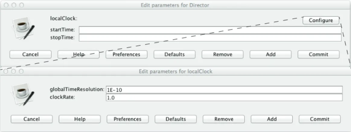
(4) 10. MODELING TIMED SYSTEMS. 10.1. Clocks. As explained in Section 1.7, Ptolemy II provides a coherent notion of time across domains. Ptolemy II supports multiform time. Every director contains a local clock that keeps track of the local time. The local time is initialized with the startTime of the director and evolves at a given clockRate. The clockRate can change. The parameter dialogue of a simple director is shown in figure 10.1 (most directors have more parameters than these, but every director has at least these). The startTime parameter, if given, specifies the time of the local clock when the model is initialized. If it is not given, then the time at initialization will be set to the time of the environment (the enclosing director, or the next director above in the hierarchy), or will be set to zero if the director is at the top level of the model. When the local time of the director reaches the value described by stopTime, the director will request to not be fired anymore (by returning false from its postfire method). The parameter dialog of a director also contains a Configure button for configuring the local clock, as shown in Figure 10.1. This can be used to set the time resolution, which is explained in Section 1.7.3, and the clock rate. The clockRate parameter specifies how rapidly the local clock progresses relative to the clock of the enclosing director. A director refers to the time of the enclosing director as the environment time. If there is no enclosing director, then advancement of the clock is entirely controlled by the director.. Figure 10.1: The director parameters for the local clock.. Ptolemaeus, System Design. 357.

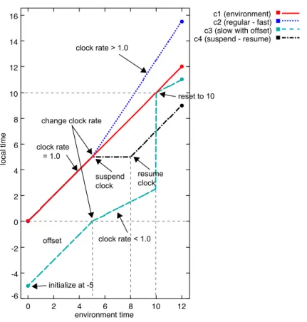
(5) 10.1. CLOCKS For example, if a DE director has an enclosing director, then the clockRate is used to translate the time stamps of input events from the environment into local time stamps. If it has no enclosing director, then all events are generated locally, and the director will always advance time to the least time stamp of unprocessed events. Every director in Ptolemy has a local clock. If an untimed director such as SDF or SR has no enclosing director, then the clock value never changes (unless its period parameter is set to a non-zero value).. Example 10.1: Figure 10.2 shows four different time lines of clocks c1 through c4. The clock c1 (solid red line) represents a clock that evolves uniformly with the environment time. Clocks c2 through c4 have varying clock rates, clock values and offsets. During the first 5 time units, all clocks evolve with the same rate as the environment time. Clock c3 starts with an offset of −5.0, i.e. it is 5 time units behind environment time. At environment time 5, the clock rates of c2 and c3 are modified; the clock rate of c2 is increased and the clock rate of c3 is decreased. Clock c4 is suspended, so that its value does not change during the next 3 time units. At time 8, c4 is resumed. At time 10, the value of c3 is set to 10 to match the environment time. Because the clock rate of c3 is still less than 1.0, the clock immediately starts lagging.. These different clock behaviors can be modeled in Ptolemy. We can perform the following actions on clocks: define an offset, change the clock value, suspend and resume the clock, and change the clock rate.. Example 10.2: The model that generates the plot shown in Figure 10.2 is presented in Figure 10.3. The clock rate is modified by changing the parameter clockRate of the parameter localClock in a director. In the Fast composite actor at the upper right, that parameter is set equal to the port parameter rate, so that each time a new rate is provided on that input port, the rate of the local clock changes. RegularToFast is a DiscreteClock actor that starts the clock with rate 1.0 at time 0.0, then changes the rate to 1.5 at time 5.0. The clock value is modified by changing the value of the parameter startTime of a director. Modifying the parameter startTime any time during the simulation will 358. Ptolemaeus, System Design.

(6) 10. MODELING TIMED SYSTEMS. set the current value of the clock to the value in the startTime parameter. The SlowWithOffset composite actor at the middle right has a port parameter called clockValue, and its director’s startTime is set to the expression clockValue to reference the port parameter. Whenever a new value arrives at that port parameter, the clock value gets set. The Offset actor at the left sets the clock to −5.0 at environment time 0.0, to 2.5 at environment time 10.0, and to 10.0, again at environment time 10.0. The latter update leverages the superdense time model in Ptolemy II to instantaneously change the clock value from one value to another, as indicated by the vertical dashed line segment in Figure 10.2.. Timed Plotter. c1 (environment) c2 (regular - fast) c3 (slow with offset) c4 (suspend - resume). 16 14. clock rate > 1.0. 12 10. reset to 10. local time. 8. change clock rate. 6. clock rate = 1.0. 4. suspend clock. 2. resume clock. 0. -4 -6. clock rate < 1.0. offset. -2. initialize at -5 0. 2. 4 6 8 environment time. 10. 12. Figure 10.2: Clocks progressing at different rates relative to environment time.. Ptolemaeus, System Design. 359.

(7) 10.1. CLOCKS. The SupendAndResume actor at the lower right is a modal model where the clock of the inside Continuous director is suspended when the state machine is not in the active state, resulting in the horizontal segment of the dash-dot line in Figure 10.2. Notice that the transition entering the active state is a history transition to prevent the local clock from being reset to its start time (if given) or the environment time (if a start time is not given). The local time of a director can be plotted by using a CurrentTime actor with the useLocalTime parameter set to true (which is the default). If the useLocalTime parameter is set to false, then the output produced will be the environment time of the top level of the model. The time lines in Figure 10.2 are obtained by periodically triggering these CurrentTime actors.. Figure 10.3: The model that generates the plot of Figure 10.2. [online]. 360. Ptolemaeus, System Design.

(8) 10. MODELING TIMED SYSTEMS. 10.2. Clock Synchronization. Many distributed systems rely on a common notion of time. A brute-force technique for providing a common notion of time is to broadcast a clock over the communication network. Whenever any component needs to know the time, it consults this broadcast clock. A well-implemented example of this is the global positioning system (GPS), which with some care can be used to synchronize widely distributed clocks to within about 100 nanoseconds. This system relies on atomic clocks deployed on a network of satellites, and careful calculations that even take into account relativistic effects. GPS, however, is not always available to systems (particularly indoor systems), and it is vulnerable to spoofing and jamming. More direct and self-contained realizations of broadcast clocks may be expensive and difficult to implement, since lack of control over communication delays can render the resulting clocks quite inaccurate. In addition, avoiding brittleness in such systems, where the source of the clock becomes a single point of failure that can bring down the entire system, may be expensive and a significant engineering challenge (Kopetz, 1997; Kopetz and Bauer, 2003). A more modern technique that improves robustness and precision is to use precision time protocols (PTP) to provide clock synchronization. Such protocols keep a network of loosely coupled clocks synchronized by exchanging time-stamped messages that each clock uses to make small corrections in its own rate of progress. This technique is more robust, because sporadic failures in communication have little effect, and even with permanent failures in communication, clocks can remain synchronized for a period of time that depends on the stability of the clock technology. This technique is also usually more precise than what is achieved by a broadcast clock; for most such protocols, the achievable precision does not depend on the communication delays, but rather instead depends on the asymmetry of the communication delays. That is, if the latency of communication from point A to point B is exactly the same as the latency of the communication from point B to point A, then perfect clock synchronization is theoretically possible. In practice, such protocols can come quite close to this theoretical limit over practical networks. The White Rabbit project at CERN, for example, claims to be able synchronize clocks on a network spanning several kilometers to under 100 picoseconds (Gaderer et al., 2009). This means that if you simultaneously ask two clocks separated by, say, 10 kilometers of networking cable, what time it is, their response will differ by less than 100 picoseconds. Over standard Ethernet-based local area networks, it is routine today to achieve precisions well under tens of nanoseconds using a PTP known Ptolemaeus, System Design. 361.

(9) 10.2. CLOCK SYNCHRONIZATION as IEEE 1588 (Eidson, 2006). Over the open Internet, it is common to use a PTP known as NTP (Mills, 2003) to achieve precisions on the order of tens of milliseconds. Typically, one or several master clocks are elected (and reelected in the event of failure), and slaves synchronize their clocks to the master by messages sent over the network. This guarantees a common notion of time across all platforms, with a well-defined error margin. The following example simulates the effects of imperfect clock synchronization.. Example 10.3: In electric power systems, a transmission line may span many kilometers. When a fault occurs, for example due to a lightning strike, finding the location of the fault may be very expensive. Hence, it is common to estimate the location of the fault based on the time that the fault is observed at each end of the transmission line. Assume a transmission line of length 60 kilometers between substation A and substation B. When a fault occurs, both substations will experience an observable event. Assuming that electricity travels through the transmission line. Figure 10.4: Line fault detection model. [online]. 362. Ptolemaeus, System Design.

(10) 10. MODELING TIMED SYSTEMS. Figure 10.5: Line fault detection — Substation A, the clock master.. Figure 10.6: Line fault detection — Substation B, the clock slave.. at a known speed, then the time difference between when substation A observes the event and substation B observes the event can be used to calculate the location of the event.. Ptolemaeus, System Design. 363.

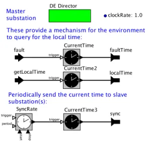
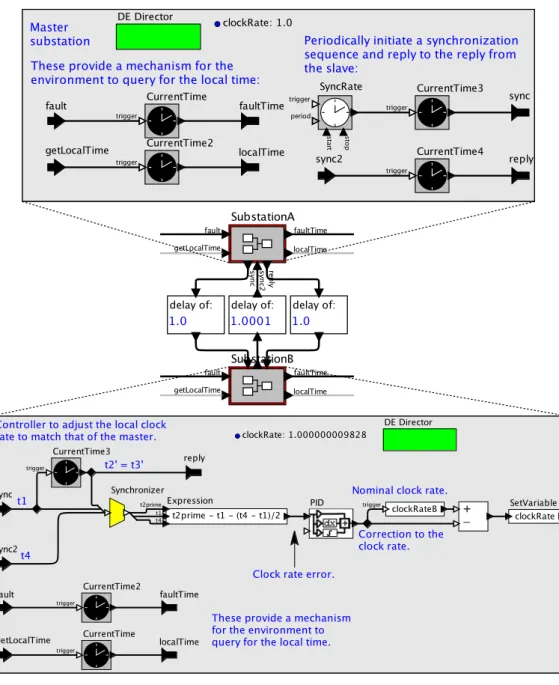
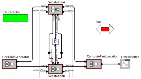
(11) 10.2. CLOCK SYNCHRONIZATION. Let X denote the location of the fault event along the transmission line (the distance from substation A). Then X satisfies the following equations, s × (TA − T0 ) = X s × (TB − T0 ) = D − X where T0 is time of fault (which is unknown), TA is the time of fault detection at substation A, TB is the time of fault detection at substation B, s is the speed of propagation along the transmission line (the speed of light), D is the distance from A to B, and D − X is the distance from B to the fault. Subtracting the above equations and solving for X yields X = ((TA − TB ) × s + D)/2. Of course, this calculation is only correct if the clocks at the two substations are perfectly synchronized. Suppose that the substations use a PTP to synchronize their clocks, and that substation A is the master. Then periodically, A and B will exchange messages that can be used to compute the discrepancy between their clocks. To see how this is done, see the sidebar on page 367 or Eidson (2006). Here, we will assume that this done perfectly (something that is only possible if the communication latency between A and B is perfectly symmetric). We focus in this model only on the effects of the control strategy that uses this information to adjust the clock of substation B. The model shown in Figure 10.4 shows SubstationA periodically sending its local time to SubstationB, where the period is given by the syncPeriod parameter, set to 20.0 seconds. In that model, the LineFaultGenerator produces faults at times 50, 100, 150, etc., and the fault is assumed to occur 20 kilometers from substation A. The substation actors send the local times at which they observe the faults to a ComputeFaultLocation composite actor, whose task it is to determine the fault location using the above formulas. Since the measured fault times arrive at the ComputeFaultLocation actor at different times, a Synchronizer is used to wait until one data value from each substation has been received before it will do a calculation. Note that inputs will be misaligned if one of the substations fails to detect the event and provide an input, so a more realistic model needs to be more sophisticated. The substation models are depicted in Figures 10.5 and 10.6. SubstationA is modeled very simply as, from top to bottom, responding to a fault input by sending the time of the fault, responding to a getLocalTime input with the local time, and periodically sending the local time to the sync output. 364. Ptolemaeus, System Design.

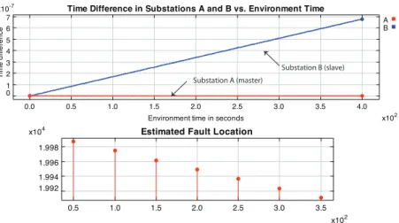
(12) 10. MODELING TIMED SYSTEMS. Substation B is a bit more complicated. When it receives a sync signal from the master, it calculates the discrepancy with its local clock; this calculation is not realistic, since there is an unknown time delay in receiving the sync signal, but PTP protocols take care of making this calculation, so this detail is not modeled here. Instead, the model focuses on what is done with the information, which is to use a PID controller to generate a correction to the local clock. The correction is added to the local clock rate and then stored in the clockRate parameter using a SetVariable actor. The director’s clock uses this same parameter for the rate of its clock, so each time a correction is made, the rate of the local clock will change. Figure 10.7 shows the simulation result. The upper plot shows the errors in the clocks. Since substation A is the master, it has no error, so its error is a constant zero. At the start of simulation, the clock of B is drifting linearly with respect to A. At 20 seconds, B receives the first sync input, and the PID controller provides a correction that reduces the rate of drift. At 40 seconds, another sync signal further reduces the rate of drift. The lower plot shows the estimated locations of the faults occurring at times 50, 100, 150, etc. The correct fault location is 20 km, so we can see that as the clocks get synchronized, the estimate converges to 20 km. Figure 10.8 shows what happens if there is no clock synchronization (the sync signal never arrives at B). In this case, the clock of B drifts linearly with respect to A, and the error in the estimated fault location grows without bound.. 10.3. Modeling Communication Delays. In design-space exploration, designers evaluate whether their designs work well on a given architecture. Part of the architecture is the communication network, which introduces delays that can affect the behavior of a system. A communication network introduces delay. It is straightforward to model constant communication delays that are independent of one another, but it is much more interesting (and realistic) to take into account shared resources, which result result in correlated and variable delays. We begin with the simpler models, and then progress to the more interesting ones. Ptolemaeus, System Design. 365.

(13) 10.3. MODELING COMMUNICATION DELAYS Time Difference in Substations A and B vs. Environment Time. Time difference. x10-4 0.2. A B. -0.0 -0.2. Substation A (master). -0.4 -0.6 -0.8 -1.0. Substation B (slave) 0.0. 0.5. 1.0. 1.5. 2.0. 2.5. Environment time in seconds. 3.0. 3.5. 3.0. 3.5. 4.0. x102. Estimated Fault Location. x104 3.0 2.5 2.0 0.5. 1.0. 1.5. 2.0. 2.5. x102. Figure 10.7: Line fault detection with clock synchronization.. Time Difference in Substations A and B vs. Environment Time. Time difference. x10-7 7 6. A B. 5 4 3. Substation B (slave). 2. Substation A (master). 1 0 0.0. 0.5. 1.0. 1.5. 2.0. 2.5. Environment time in seconds. 3.0. 3.5. 3.0. 3.5. 4.0. Estimated Fault Location. x104. x102. 1.998 1.996 1.994 1.992 0.5. 1.0. 1.5. 2.0. 2.5. x102. Figure 10.8: Line fault detection without clock synchronization.. 366. Ptolemaeus, System Design.

(14) 10. MODELING TIMED SYSTEMS. Sidebar: Precision Time Protocols The figure at the right shows how a typical PTP works. The clock master A initiates an exchange of messages. The first message is sent at time t1 (by the master clock) and contains the value of t1 . That message is received by the slave B at time t2 (by the master clock), but since the slave does not have access to the master clock, the slave records the time t02 that it receives the message according to its own clock. If its clock is off by e vs. the master clock, then t02 = t2 + e.. master A t1. slave B t1. t2+e t3+e. t4 t4. The slave responds by sending a message back to the master at time t03 according to its clock, or t3 according to the master’s clock, so t03 = t3 + e. The master receives this second message at t4 , and replies with a third message containing the value of t4 . The slave now has t1 , t02 , t03 , and t4 . Now notice that the round trip communication latency (the time that a message from A to B and a reply message spend in transport) is r = (t2 − t1 ) + (t4 − t3 ) = (t4 − t1 ) − (t3 − t2 ). At B, this value can be calculated even though t2 and t3 are not known, because (t3 − t2 ) = (t03 − t02 ), and slave B has t02 , and t03 . If the communication latencies are symmetric, then the one way latency is r/2. To correct the clock of B, we simply need to estimate e. This will tell us whether the clock is ahead or behind, so we can slow it down or speed it up, respectively. If the communication channel has symmetric delays (i.e. t2 − t1 = t4 − t3 ), then a very good estimate is given by e˜ = t02 − t1 − r/2. In fact, if the communication latency is exactly symmetric, then e˜ = e, the exact clock error. B can now adjust its local clock by e˜. Ptolemaeus, System Design. 367.

(15) 10.3. MODELING COMMUNICATION DELAYS. 10.3.1. Constant and Independent Communication Delays. In the DE domain, network delays that are independent of one another can be easily modeled using the TimeDelay actor.. Example 10.4: The line fault detector of Figure 10.4 idealizes the calculation of the clock error in substation B. In practice, calculating clock discrepancies is not trivial. A typical technique implemented in a PTP is described in the sidebar on page 367 and implemented in the model in Figure 10.9. In Figure 10.9, substation A periodically initiates a sequence of messages that are used to calculate the clock discrepancy. First, at master time t1 , it sends the value of this time to substation B. Substation B responds. Substation A responds to the response with the time t4 that it receives the response. When substation B has received this final message, it has enough information to estimate the discrepancy between its clock and that of the master. The Synchronizer actor ensures that this estimate is only calculated after all the requisite information has been received. Figure 10.9 has three TimeDelay actors that can model network latency in the communication of synchronization messages. Interestingly, if all three delays are set to the same value, even a rather large value such as 1.0 seconds, then the performance of the model in identifying the location of the fault is essentially identical to that of the idealized model. However, if, as shown, one of the delays is changed only slightly, to 1.0001, then the performance degrades considerably, as shown in Figure 10.10. The slave clock settles into a substantial steady-state error, and the estimated fault location converges to approximately 13 kilometers, quite different from the actual fault location at 20 kilometers. Clearly, if the communication channel is expected to be asymmetric, then the designer has work to do to improve the control algorithm. A different choice of parameters for the PID controller would probably help, but perhaps at the expense of lengthening the convergence time.. 10.3.2. Modeling Contention for Shared Resources. In the model in Figure 10.9, each connection between actors has a fixed communication delay. This is not very realistic for practical communication channels, where the delay 368. Ptolemaeus, System Design.

(16) 10. MODELING TIMED SYSTEMS. Figure 10.9: Line fault detection with communication delays in the PTP implementation. [online]. Ptolemaeus, System Design. 369.

(17) 10.3. MODELING COMMUNICATION DELAYS Time Difference in Substations A and B vs. Environment Time. Time difference. x10-5 8 6 4 2 0 -2 -4 -6. A B. Substation B (slave). Substation A (master) 0.0. 0.5. x10. 1.0. 1.5. 2.0. 2.5. Environment time in seconds. 3.0. 3.5. 3.0. 3.5. 4.0. x102. Estimated Fault Location. 4. 2.5 2.0 1.5 1.0 0.5. 1.0. 1.5. 2.0. 2.5. x102. Figure 10.10: Line fault detection performs poorly with PTP when network latencies are asymmetric.. will depend on other uses of the channel. Most communication channels have shared resources (radio bandwidth, wires, buffer space in routers, etc.), and the latency through the network can vary significantly depending on other uses of these resources. The model in Figure 10.9 could be modified to route all the messages through a single, more elaborate network model. However, this leads to considerable modeling complexity. Suppose for example that we wish to model the network using a single Server actor, perhaps the most basic model for a shared resource. Then all messages that traverse the channel would have to be merged into a single stream to feed to the Server actor. These streams would then have to be separated after emerging from the Server actor, so destination addresses would have to be encoded in the messages before the streams are merged. The model suddenly becomes very complicated. Fortunately, Ptolemy II has a much cleaner mechanism for handling shared resources. We use aspect-oriented modeling (AOM), which is based on aspect-oriented programming (Kiczales et al., 1997), to map functionality to implementation. This way of associating functional models with implementation models and schedulers was introduced in Metropolis (Balarin et al., 2003), where the mechanism was called a quantity manager. In Ptolemy II, an aspect is an actor that manages a resource; it is associated with the actors and ports that share the resource. In a simulation run, the aspect actor schedules the 370. Ptolemaeus, System Design.

(18) 10. MODELING TIMED SYSTEMS use of the resource. The association between the resource and the users of the resource is done via parameters, not by direct connections through ports. As a consequence, aspects are added to an existing model without changing the interconnection topology of the existing model. The next example shows how communication aspects can be used to cleanly model shared communication resources.. Example 10.5: Figure 10.11 shows a variant of the line fault detector model where we have dragged into the model a communication aspect called Bus. In this example, the PTP communications between SubstationA and SubstationB use the shared bus. This is indicated in the figure by the annotation “Aspects: Bus” on the input ports, and by red fill in the port icon. The Bus has a serviceTime parameter that specifies the amount of time that it takes a token to traverse the channel. During that time, the Bus is busy, so any further attempts to use the Bus will be delayed. The Bus therefore acts like a Server actor with an unbounded buffer, but since it is an aspect, there is no need for the model to explicitly show all the communication paths passing through a single instance of a Server.. Figure 10.11: Line fault detection where communication uses a shared bus, modeled using a communication aspect. [online]. Ptolemaeus, System Design. 371.

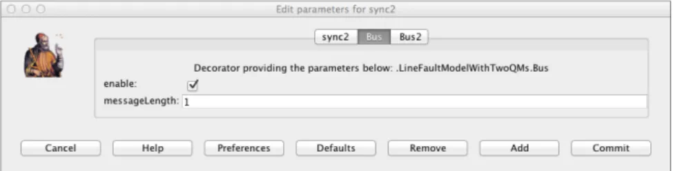
(19) 10.3. MODELING COMMUNICATION DELAYS. In this example, the communications latencies are symmetric, because there is no contention for the bus. Hence, the line fault detection algorithm performs well, behaving similarly to Figure 10.7. If, on the other hand, you enable use of the bus for other communication paths in the model, such as at the input ports of ComputeFaultLocation, then the performance will degrade considerably, because contention for the bus will introduce asymmetries in the communication latencies.. To use an aspect for modeling communication, simply drag one into the model from the library and assign it a meaningful name. The Bus, along with several others that are (as of this writing) still rather experimental, can be found in the MoreLibraries→Aspects library. An aspect is a decorator, which means that it endows elements of the model with parameters (see sidebar on page 373). In the case of the Bus, it decorates ports with an enable and messageLength parameter, as shown in Figure 10.12. When an input port has the Bus enabled, then messages sent to that input port will be delayed by at least the product of the messageLength parameter of the port and the serviceTimeMultiplicationFactor parameter of the Bus. The delay is at least this, because if the bus is busy when the message is sent, then the message has to wait until the bus becomes free. You can add any number of aspects to a model. Each is a decorator, and each can be independently enabled. If an input port enables multiple communication aspects, then. Figure 10.12: The Bus aspect decorates ports with an enable and messageLength parameter. This figure shows a parameter editor for a port in model in Figure 10.14, which has two busses.. 372. Ptolemaeus, System Design.

(20) 10. MODELING TIMED SYSTEMS those aspects mediate the communication in the order in which the aspects are enabled. Hence, aspects may be composed.. Example 10.6: In Figure 10.14, a second bus has been added to the model, and the communication from SubstationB to SubstationA traverses Bus and Bus2, in that order, as you can see from the annotation on the sync2 input port to SubstationA. As a consequence, the communication latencies become asymmetric, and the line fault detection algorithm performs poorly, yielding results similar to those in Figure. Sidebar: Decorators A decorator in Ptolemy II is an object that adds to other objects in the model parameters, and then uses those parameter values to provide some service. The simplest decorator provided in the standard library is the ConstraintMonitor, which can be found in the Utilities→Analysis library. The ConstraintMonitor is an attribute that, when inserted in model, adds a parameter called value to actors in the model. The ConstraintMonitor keeps track of the sum of all the values that are set for actors in the model, displays that sum in its icon, and compares that sum against a threshold. An example use of ConstraintMonitor is shown in Figure 10.13, where a ConstraintMonitor has been dragged into a model with three actors and renamed “Cost.” Once that ConstraintMonitor is in the model, then the parameter editing window for each actor acquires a new tab, as shown at the top of the figure, where the label on the tab matches the name of the ConstraintMonitor. The user can enter a cost for each actor in the model, and the ConstraintMonitor will display the total cost in its icon. The ConstraintMonitor has a parameter threshold, which specifies a limit on the sum of the values. When the total approaches the limit, the color of the ConstraintMonitor icon changes to yellow. When the total hits or exceeds the limit, if the warningEnabled parameter is true, then the user is warned. The default value for threshold is Infinity, which means no limit. The ConstraintMonitor has two other parameters, as shown at the bottom of Figure 10.13. If includeOpaqueContents is true, then actors inside opaque composite actors will also be decorated. Otherwise, they will not be decorated. If includeTransparents is true, then transparent composite actors will be decorated. Otherwise, they will not be. There are many other uses for decorators. A director can be a decorator. The aspects described in this chapter are decorators. Ptolemaeus, System Design. 373.

(21) 10.3. MODELING COMMUNICATION DELAYS. Figure 10.13: A decorator in Ptolemy II is an object that adds to other objects in the model parameters, and then uses those parameter values to provide some service. In this example, a ConstraintMonitor (which has been renamed Cost) is monitoring the total cost of components in the model, checking them against a threshold of 100.0. 374. Ptolemaeus, System Design.

(22) 10. MODELING TIMED SYSTEMS. 10.10. The decoratorHighlightColor parameter of Bus2 has been changed from red to green, resulting in green highlighting of both the port and the bus icon.. 10.3.3. Composite Aspects. The aspects discussed in the previous section are like atomic actors; their logic is defined in a Java class. For a more flexible way of describing communication aspects, we use the CompositeCommunicationAspect. This actor can be found in Ptolemy under MoreLibraries→Aspects.. Example 10.7: Figure 10.15 shows the bus example implemented using a CompositeQuantityManager. In this case, the bus behavior is modeled using a discreteevent subsystem with a Server actor. Requests to use the bus queue up at the input. Figure 10.14: Line fault detection where one of the communications traverses two busses, yielding asymmetric communication. [online]. Ptolemaeus, System Design. 375.

(23) 10.3. MODELING COMMUNICATION DELAYS. Figure 10.15: A bus implemented as a composite communication aspect. [online]. to the server. When the server becomes free, the first queued input is delayed by the serviceTime. The behavior is identical to that of the atomic Bus aspect.. Since a composite communication aspect is simply a Ptolemy II model, we have a great deal of freedom in its design.. Example 10.8: In the example of Figure 10.15, the bus is being used not only for the communication between SubstationA and SubstationB, but also in the communication to the ComputeFaultLocation actor. Contention for the bus makes the communication latencies asymmetric, degrading the performance of the clock syn376. Ptolemaeus, System Design.

(24) 10. MODELING TIMED SYSTEMS. Figure 10.16: A network that reduces contention implemented as a composite aspect. At the bottom is shown how the decorator parameters of a port are used to select the port of the aspect that handles the communication. [online]. Ptolemaeus, System Design. 377.

(25) 10.4. MODELING EXECUTION TIME. chronization, and resulting in very poor performance in computing the fault location. We can improve the performance with a better network, as shown in Figure 10.16. In that figure, we have modified the Bus so that it is now a more sophisticated network with two input ports and two distinct servers. By routing communication to the two servers, contention can be reduced. Each input port involved in a communication specifies which input port, in1 or in2, of the aspect should handle the communication. At the bottom of the figure is shown how the decorator parameters of a port are used to select the port of the aspect that handles the communication. In the figure, the top input port of ComputeFaultLocation is using in2. If the bottom port also uses in2, and the ports handling the communication between SubstationA and SubstationB use in1, then contention is reduced enough to deliver excellent performance, similar to that in Figure 10.7.. 10.4. Modeling Execution Time. In addition to modeling network characteristics such as communication delays, one might also want to model execution time, the time it takes it takes an actor to perform its function on a particular implementation platform. The joint modeling of an application’s functionality and its performance on a model of the implementation platform is a very powerful tool for design-space exploration. It makes it much easier to understand the impact of choices in networking infrastructure and processor architecture. In a discrete-event model, execution times can be simulated using a Server actor for each execution resource (such as a processor), where the service time is the execution time. Example 7.5 and Figure 7.8 illustrate this for a simple storage system. However, such models are difficult to combine with models of complex functionality. Fortunately, Ptolemy provides execution aspects, which, like communication aspects, provide a form of aspect-oriented modeling. Execution aspects can be used to model contention for resources that are required to execute an application model. The mechanisms are similar to those of the communication aspects, as illustrated in the next example.. 378. Ptolemaeus, System Design.

(26) 10. MODELING TIMED SYSTEMS. Figure 10.17: A model with two alternative execution aspects, one that models a one-processor execution platform and one that models a two-processor execution platform. [online]. Ptolemaeus, System Design. 379.

(27) 10.5. PTIDES FOR DISTRIBUTED REAL-TIME SYSTEMS. Example 10.9: A variant of the generator model considered in Section 1.9 is shown in Figure 10.17. This model includes two possible implementation platforms, one with one processor, one with two processors, shown at the bottom of the figure. These two implementation platforms are modeled using the CompositeResourceScheduler actor, found in MoreLibraries→ResourceScheduler. In this model, the Supervisor and Controller actors execute on one of the two processor architectures. Which one is determined by the value of the useTwoProcessors parameter in the model. If the value of this parameter is true, then the 2Processor aspect will be used to execute Supervisor and Controller. Otherwise, 1Processor will be used. When this model is executed, the behavior changes with the value of useTwoProcessors. When two processors are used, there is no contention for resources, since Supervisor and Controller can execute simultaneously, as modeled by the two Server actors at the lower right in the figure. However, when only one processor is used, the Supervisor and Controller compete for the use a single processor, as modeled by the single server at the lower left. In that case, there is more delay in one of the two feedback loops, which changes the dynamics of the model. In particular, with certain choices of parameters and test conditions, the choice of processor architecture could affect whether the over voltage protection conditions shown in the plot in Figure 1.11 occurs. Notice the use of RecordDisassembler actors in the composite execution aspects. The input to the submodel in the composite aspect is a record that contains the values of the decorator parameter executionTime of the actor requesting an execution resource. This execution time is extracted from the record and becomes the service time of the Server.. 10.5. Ptides for Distributed Real-Time Systems. So far, this chapter has focused on modeling and simulating timing behavior in system implementations. Another role for timed models, however, is to specify timing behavior. That is, a timed model may give the required behavior of an implementation without 380. Ptolemaeus, System Design.

(28) 10. MODELING TIMED SYSTEMS completely describing the implementation. Towards this end, we focus for the remainder of this chapter on a programming model for distributed real-time systems called Ptides.∗ Ptides models are designed to solve the problem identified in Example 10.9 above, where the behavior of a system depends on the details of the hardware and software platform that executes the system. A key goal in Ptides is to ensure that every correct execution of a system delivers exactly the same dynamic behavior.. Example 10.10: In Example 10.9, choosing to execute Supervisor and Controller on a single processor yields different dynamic behavior than choosing two processors. If these were Ptides models, the two behaviors would be identical, as long as the processor resources were sufficient to deliver a correct execution. Moreover, the execution times of the Supervisor and Controller will also not affect the dynamics until they get so large that a correct execution is no longer possible. Hence, Ptides has the potential to reduce the sensitivity that a system has to implementation details. Behavior is exactly the same over a range of implementations.. A Ptides model is a DE model with certain constraints on time stamps. Ptides is used to design event-triggered distributed real-time systems, where events may be occurring regularly (as in sampled-data systems) or irregularly. A key idea in Ptides is that, unlike DE, time stamps have a relationship with real time at sensors and actuators (which are the devices that bridge the cyber and the physical parts of cyber-physical systems). A second key idea in Ptides is that it leverages network time synchronization (Johannessen, 2004; Eidson, 2006) to provide a coherent global meaning to time stamps in distributed systems. The most interesting, subtle, and potentially confusing part about Ptides is the relationship between multiple time lines. But herein also lies its power.. 10.5.1. Structure of a Ptides Model. A Ptides model consists of one or more Ptides platforms, each of which models a computer on a network. A Ptides platform is a composite actor that contains actors representing sensors, actuators, and network ports, and actors that perform computation and/or ∗. The name comes from the somewhat tortured acronym for “programming temporally integrated distributed embedded systems.” The initial “P” is silent, as in Ptolemy, so the name is pronounced “tides.”. Ptolemaeus, System Design. 381.

(29) 10.5. PTIDES FOR DISTRIBUTED REAL-TIME SYSTEMS. Sidebar: Background of Ptides Ptides leverages network time synchronization (Johannessen, 2004; Eidson, 2006) to provide a coherent global temporal semantics in distributed systems. The Ptides programming model was originally developed by Yang Zhao as part of her Ph.D. research (Zhao et al., 2007; Zhao, 2009). Zhao showed that, subject to assumed bounds on network latency, Ptides models are deterministic. The case for a time-centric approach like Ptides is elaborated by Lee et al. (2009b), and an overview of Ptides and an application to power-plant control is given by Eidson et al. (2012), A number of implementations followed the initial work. A simulator is described by Derler et al. (2008), and an execution policy suitable for implementation in embedded software systems by Feng et al. (2008) and Zou et al. (2009b). Zou (2011) developed PtidyOS, a lightweight microkernel implementing Ptides on embedded computers, and a code generator producing embedded C programs from models. Matic et al. (2011) adapted PtidyOS and the code generator to demonstrate their use in smart grid technologies. Feng and Lee (2008) extended Ptides with incremental checkpointing to provide a measure of fault tolerance. They showed conditions under which rollback can recover from errors, observing that the key constraint in Ptides is that actuator actions cannot be rolled back. Ptides has also been used to coordinate real-time components written in Java (Zou et al., 2009a). A technique similar to Ptides was independently developed at Google for managing distributed databases (Corbett et al., 2012). In this work, clocks are synchronized across data centers, and messages sent between data centers are time stamped. The technique provides a measure of determinacy and consistency in database accesses and updates. Assuming that the network latency bounds are met, a correct implementation of Ptides is deterministic in that a sequence of time-stamped events from sensors always results in a unique and well-defined sequence of time-stamped events delivered to actuators. However, this determinism does not provide any guarantee that events are delivered to actuators on time (prior to the deadline given by the time stamp). The problem of determining whether events can be delivered on time to actuators is called the schedulability problem. The question is, given a Ptides model, does there exist a schedule of the firing of actors such that deadlines are met. Zhao (2009) solved this problem for a limited class of models. The problem is further discussed by Zou et al. (2009b), and largely solved by Matsikoudis et al. (2013). 382. Ptolemaeus, System Design.

(30) 10. MODELING TIMED SYSTEMS. Figure 10.18: Ptides model with two Ptides platforms, sensor, actuator and network ports. [online]. modify time stamps. A Ptides platform contains a PtidesDirector and represents a single device in a distributed cyber-physical system, such as a circuit board containing a microcontroller and some set of sensor and actuator devices. For simulation purposes, a Ptides platform is placed within a DE model that models the physical environment of the platform.. Ptolemaeus, System Design. 383.

(31) 10.5. PTIDES FOR DISTRIBUTED REAL-TIME SYSTEMS. Example 10.11: A simple Ptides model is shown in Figure 10.18. This model has two platforms connected to a physical plant (via sensors and actuators) and to a network. The top-level director is a DE director, whereas the platform directors are Ptides directors. The physical plant may internally be a Continuous model.. Ptides models leverage Ptolemy’s multiform time mechanism. A common pattern in such models assumes the time line at the top-level of the model hierarchy represents an idealized physical time line that advances uniformly throughout the system. This time line cannot be directly observed by computational devices in the network, which must instead use clocks to approximately measure it. We refer to such an idealized time at the top level as the oracle time. In the MARTE time library, the same idealized concept of physical time is referred to simply as ideal time (Andr´e et al., 2007). Within a platform, a local clock maintains a time line called platform time, which approximates oracle time. Platform time is chronometric, an imperfect measurement of oracle time. The builder of a Ptides model may choose to assume that platform time perfectly tracks oracle time or, more interestingly, to model imperfections in tracking and discrepancies across the network, as illustrated in Section 10.2 above.. Example 10.12: In the Ptides model of Figure 10.18, the top-level director’s clock represents oracle time. The clocks of the Ptides directors represent platform time. These can be parameterized to drift with respect to each other and platform time and to have offsets.. A key innovation in Ptides, however, is that a second time line called logical time plays a key role in a platform. The notion of logical time in distributed systems was introduced by Lamport et al. (1978), and is applied in Ptides to achieve determinism in distributed realtime systems. Any actor that requests the current time from the PtidesDirector will be told about logical time, not about platform time. The only actors that have access to platform time are sensors, actuators, and network interfaces, i.e. the actors at the cyber-physical boundary. Specifically, when a sensor produces an event in a Ptides model, the time stamp of the event is a logical time value equal to the platform time at which the sensor takes its 384. Ptolemaeus, System Design.

(32) 10. MODELING TIMED SYSTEMS measurement. That is, Ptides binds logical time to physical time (as measured by platform time) at sensors.. Example 10.13: In the Ptides model of Figure 10.18, the sensor uses the platform time of PtidesPlatform1 to construct a time stamp for each event that it produces. Such an event represents a measurement made on the physical plant, and its (logical) time stamp is equal to the local measurement of time.. Let ts be the platform time at which a measurement is made by a sensor. The event produced by that sensor actor will have logical time stamp ts . A TimeDelay actor, however, operates in logical time. It simply manipulates the logical time stamp. Platform time is not visible to it. If an input to a TimeDelay actor whose delay value is d1 has (logical) time stamp t, then its output will have time stamp t + d1 . Once an event from a sensor has been produced, it is processed by the Ptides model like any other discrete event in a DE system. That is, events with logical time stamps are processed by the PtidesDirector in time-stamp order, without particular concern for platform time or oracle time. Actors are fired as they would be in simulation. A key property of Ptides models is that this time-stamp-ordered processing of events is preserved despite the distributed architecture and imperfect clocks. This key property delivers determinism. An actuator port inside a Ptides platform acts as an output from the platform. When it receives an event from the platform Ptides model, that event has a logical time stamp t. The actuator interprets t as a deadline relative to platform time. That is, an event with time stamp t sent to an actuator is a command to perform some physical action no later than the (platform) time equal to t. Hence, actuators, like sensors, also bridge logical and physical times.. Example 10.14: In the Ptides model of Figure 10.18, in PtidesPlatform1, assume the SensorPort produces an event with time stamp ts . This represents the platform time at which a sensor measurement is made. Assume further that Computation is a zero-delay actor, and that it reacts to the event from SensorPort by producing an output event with the same time stamp ts . The output of the TimeDelay actor, therefore, will have time stamp ts + d1 , where d1 is the delay of the TimeDelay Ptolemaeus, System Design. 385.

(33) 10.5. PTIDES FOR DISTRIBUTED REAL-TIME SYSTEMS. actor. That event goes to the ActuatorPort, which interprets the time stamp ts + d1 as a deadline. That is, the actuator should produce its actuation at platform time no later than ts + d1 .. By default, when executing a Ptides model, actors are assumed to be instantaneous (in platform time). Hence, the deadline at ActuatorPort in Figure 10.18 will never be violated. In fact, in the simulation, the ActuatorPort will be able to perform its actuation as early as platform time ts . This is not very realistic, because any physical realization of this platform will incur some latency. It cannot react instantaneously to sensor events. More realistic simulation models can be constructed by combining the execution aspects of Section 10.4 with Ptides, but we will not do that here. Instead, here, we will assume that there is some variability in the latency introduced by the physical realization of the platform, but that the deadline will nevertheless be met. Verifying this is a schedulability problem. The actuation of ActuatorPort in Figure 10.18 affects the physical plant, which in turn affects the SensorPort. There is a feedback loop, and the closed-loop behavior will be affected by the latency of the platform. If that latency is unknown or variable, then the overall closed-loop behavior of the system will be unknown or variable, yielding a nondeterministic model. To regain determinism, Ptides actuators can be configured to perform their actuation at the deadline rather than by the deadline. As long as events arrive at or before the deadline, the actuator will be able to produce its actuation deterministically, independent of the actual arrival time of the events, and hence independent of execution time variability. The response of PtidesPlatform1 to a sensor event will a deterministic actuator event (in platform time and oracle time). This makes the behavior of the entire closed-loop system independent of variability in execution times (and, as we will show below, network delays). To configure a Ptides actuator to provide this determinism, set the actuateAtEventTimestamp parameter of the ActuatorPort to true. Ptides, therefore, provides a mechanism to hide underlying uncertainty and variability (up to a failure threshold, when deadlines are not met), yielding deterministic closed-loop behavior. A natural question arises now about what to do if the failure threshold is crossed. By default, an actuator port in Ptides will throw an exception if it receives an event with time stamp t and platform time has already exceeded t. Such an exception is an indication that assumptions about the ability of the platform to meet the deadline have been violated. A well-designed model will catch such exceptions, using for example error transitions in a modal model (see Section 8.2.3). How to handle such exceptions, of course, is application 386. Ptolemaeus, System Design.

(34) 10. MODELING TIMED SYSTEMS dependent. It might be necessary, for example, to switch to a safe but degraded mode of operation. Or it might be necessary to restart some portion of the system, or to switch to a backup system. Multiple Ptides platforms in a model may communicate via a network. When such communication occurs, logical time stamps are conveyed along with the data. Unlike an actuator port, a network transmitter port always produces its output immediately when it becomes available, rather than waiting for platform time to match the time stamp. The logical time stamp of the event will be carried along with the event to the network receiver port, which will then produce on its output an event with that same time stamp. Like an actuator port, a network transmitter port treats the time stamp as a deadline and will throw an exception if the platform time exceeds the time stamp value when the event arrives.†. Example 10.15: In the Ptides model of Figure 10.18, in PtidesPlatform1, assume that the sensor makes a measurement at platform time ts , and that consequently the network transmitter port receives an event with time stamp ts + d1 . Assume further that it receives this event at platform time ts , because the execution time of actors is (by default) assumed to be zero. Hence, the Network actor in Figure 10.18 will received an event containing as its payload both a value (the value of the event delivered to the NetworkTransmitterPort) and a logical time stamp ts + d1 . The NetworkTransmitterPort will launch this payload into the network at platform time ts . The network will incur some delay, simulated by the Network actor in the figure, and will arrive at PtidesPlatform2 at some time t2 , a local platform time at PtidesPlatform2. The NetworkReceiverPort on PtidesPlatform2 will produce an output event with (logical) time stamp ts + d1 , extracted from the payload. In Figure 10.18, this event will pass through another Computation actor and another TimeDelay actor. Assuming the TimeDelay actor increments the time stamp by d2 , the ActuatorPort on PtidesPlatform2 will receive an event with time stamp ts + d1 + d2 . This deadline will be met if ts + d1 + d2 ≥ t2 . If the actuateAtEventTimestamp parameter of the ActuatorPort is true, and all deadlines are met, then the overall latency from the sensor in platform 1 to the actuator in platform 2 is deterministic and independent of the actual network delay †. This deadline may be modified to be earlier or later by changing the platformDelayBound parameter of the network transmitter port, as explained below.. Ptolemaeus, System Design. 387.

(35) 10.5. PTIDES FOR DISTRIBUTED REAL-TIME SYSTEMS. and actual computation times. This ability to have a fixed latency in a distributed system is central to the power of the Ptides model.. As with the actuator on platform 1, if the deadline is not met at the actuator on platform 2, the ActuatorPort will throw an exception. This exception is an indication that some timing assumption about the implementation has been violated; for example, an assumed bound on the network latency has not been actually met by the network. This should be handled by the model as an error condition, which could, for example, cause the model to switch into a safe but degraded mode of operation. Although the end-to-end latency from the sensor on platform 1 to the actuator on platform 2 is deterministic, it is not exactly clear from this model what that latency is. Nominally, the latency is the logical time delay, d1 + d2 . However, the time at which the actuation occurs, ts + d1 + d2 , is relative to the local platform clock at platform 2. This time, however, also depends on the clock on platform 1, since ts is the time on platform 1 when the sensor measurement is taken. Hence, to be useful, a distributed Ptides system requires that clocks be synchronized (see Section 10.2). They need not be perfectly synchronized, but if the error between them is not bounded, then there is no bound on the end-to-end latency (in oracle time). If these two platform clocks are perfectly synchronized, then the actual latency will be exactly d1 + d2 , relative to these platform clocks. The latency in oracle time, of course, depends on the drift of these clocks relative to oracle time (see Figure 10.2). If these two clocks progress at exactly the rate of oracle time, then the actual latency will be exactly d1 + d2 in oracle time. Hence, with sufficiently good clocks and sufficiently good clock synchronization, Ptides gives an overall timing behavior that is precise and deterministic up to the precision of these clocks. To help ensure that a realization meets the requirements of a specification, a network receiver port also imposes a constraint on timing. As mentioned above, the network transmitter port will throw an exception if it receives an event at a platform time greater than the time stamp of the event.‡ So if a network receiver port receives a message, it knows that the message was transmitted at a platform time no later than the time stamp on the message it receives. The receiver has a parameter networkDelayBound, which is an upper bound on the network delay that it assumes. When the network receiver receives a ‡. This deadline may be modified to be earlier or later by changing the platformDelayBound parameter of the network transmitter port, as explained below.. 388. Ptolemaeus, System Design.

(36) 10. MODELING TIMED SYSTEMS message, it checks that the platform time does not exceed the time stamp on the message plus the networkDelayBound plus a fudge factor to account for clock discrepancies and device delays, which also have assumed bounds specified by parameters, described below. If the platform time is too large, then the network receiver knows that one of these assumptions was violated (though it cannot know which one), and it throws an exception. Although this constraint is very subtle, the consequences on models are relatively easy to understand.. Example 10.16: In the Ptides model of Figure 10.18, along the path from the sensor to the network receiver port, there cannot be a physical delay greater than the logical delay along the same path. The logical delay along this path is simply d1 , the parameter of the TimeDelay actor. The physical delay is the sum of the executions times of the actors along the path (which in simulation is assumed to be zero by default) and the network delay. Hence, if the network imposes a delay greater than d1 , the model in this figure will fail with an exception (by default, though other error handling strategies are also possible).. Notice that if we were to replace the Ptides directors in the platforms with DE directors, then the behavior would be significantly different. In this case, the latency from the sensor in platform 1 to the actuator in platform 2 would include the actual network delay. A key property of Ptides is that network delays and computation times are segregated from the logical timing of a model. The logical timing becomes a specification of timing behavior, whereas network delays and computation times are part of the realization of the system. Ptides models enable us to determine conditions under which realizations will meet the requirements of the specification. And the simulator enables evaluation of behavior under elaborate conditions that would be very difficult to validate analytically, for example taking into account the complicated dynamics of PTP clock synchronization protocols.. 10.5.2. Ptides Components. Ptides ports. Ports in a Ptides platform represent devices that communicate with the environment or the network. Ptides ports can model device delays, although by default these delays are zero. Every Ptides port has a deviceDelay and a deviceDelayBound parameter. The deviceDelay d models delay of the device. For example, if a sensor makes a meaPtolemaeus, System Design. 389.

(37) 10.5. PTIDES FOR DISTRIBUTED REAL-TIME SYSTEMS. Sidebar: Safe-to-Process Analysis The execution of actors inside a Ptides platform follows DE semantics. Actors must process events in time-stamp order (unless they are memoryless). In simulation, it is straightforward to ensure that events are processed in time-stamp order, but when Ptides models are deployed, things get more complicated. In particular, a deployed system cannot easily coordinate the scheduling of actor firings across platforms. Each platform must be able to make its own scheduling decisions. Consider the platform model shown in Figure 10.19. This example has a sensor port and a network receiver port. Suppose that the sensor produces an event with time stamp ts . If we assume that every sensor produces events in time-stamp order, then the scheduler can immediately fire Computation1. Suppose that firing produces another event with time stamp ts , which then results in an event with time stamp ts + d1 available at the top input of Computation3. When can Computation3 be fired to react to that event? The scheduler has to be sure that no event with time stamp less than or equal to ts + d1 will later become available at the bottom input of Computation3. A simple approach, developed by Chandy and Misra (1979) for distributed DE simulation, is to wait until there is an event available on the bottom input of Computation3 with time stamp greater than or equal to ts + d1 . But this could result in quite a wait, particularly if a fault occurs and the source of events on this path fails. An alternative approach due to Jefferson (1985) fires Computation3 speculatively, assuming no problematic event will later arrive, and if it does, reverses the computation by restoring the state of the actor. This approach is fundamentally limited by the inability to backtrack actuators. The Ptides approach ensures that events are processed in order as long as all deadlines are met. In our example, an event at the top input of Computation3 with time stamp ts + d1 can be safely processed when the local platform time meets or exceeds ts + d1 . This is because schedulability requires that an event with time stamp ts + d1 or earlier is required to arrive at the network receiver port at platform time ts + d1 or earlier. Conversely, suppose an event with time stamp tn is at the bottom input of Computation3. That event is safe to process when platform time meets tn − d1 + s, where s is a bound on the sensor delay, the time between a sensor event time stamp and the event becoming visible to the scheduler. See page 382 for citations that explain safe-to-process analysis in more detail. 390. Ptolemaeus, System Design.

(38) 10. MODELING TIMED SYSTEMS. Figure 10.19: Simple Ptides example used to illustrate safe-to-process analysis.. surement at platform time ts , it will produce an event with time stamp ts . But that event will not appear until platform time ts + d. For example, d might represent the amount of platform time that it takes for the sensor device to raise an interrupt request, and for the processor to respond to the interrupt request. The deviceDelayBound dB gives an upper bound on the deviceDelay d. The Ptides framework assumes that deviceDelay can vary during execution but will never exceed deviceDelayBound, which does not vary. This bound is used in safe to process analysis (see sidebar on page 390), which ensures that events are processed in time-stamp order. Sensors. A sensor port is a particular kind of Ptides port that looks like this:. It receives inputs from the environment and creates new events with the time stamp equal to the current platform time (which is the current local time of the PtidesDirector) and posts this event on the event queue. An event that is received by a sensor at platform time ts is produced with logical time stamp ts at platform time ts + d.. Ptolemaeus, System Design. 391.

(39) 10.5. PTIDES FOR DISTRIBUTED REAL-TIME SYSTEMS Actuators. An actuator port is a particular kind of Ptides port that looks like this:. By default, an actuator port produces events on the output of the platform when the time stamp of the event equals the current platform time. If you change actuateAtEventtimestamp to false, then the event may be produced earlier if it is available earlier. The deviceDelayBound parameter specifies a setup time for the device. Specifically, the deadline for delivery of an event with time stamp t to an actuator is platform time t − dB , where dB is the value of deviceDelayBound. An exception is thrown if this deadline is not met. Network transmitters and receivers. Network transmitter ports and network receiver ports are also particular kinds of Ptides port that look like this:. The NetworkTransmitterPort takes an event from the inside of the Ptides platform and sends to the outside a record that encodes the time stamp of the event and its value (the payload). The NetworkReceiverPort extracts the time stamp and the payload and produces at the inside of the destination Ptides platform and event with the specified value and time stamp. The parameter networkDelayBound (dN ) specifies the assumed maximum amount of time an incoming token spends in the network before it arrives at the receiver. It is used to determine whether an event can processed safely, or whether another event with a smaller time stamp may still be in the network. If the actual network delay exceeds this bound and the delay causes the message to be received too late, then the network receiver port will throw an exception. 392. Ptolemaeus, System Design.

(40) 10. MODELING TIMED SYSTEMS. 10.6. Summary. Modeling of complex timed systems is not easy. We all harbor a naive notion of a uniform fabric of time, shared by all participants in the physical world. But such a notion is a fiction, and real systems are strongly affected by errors in time measurement and discrepancies between logical and physical notions of time. A major focus of recent work in the Ptolemy Project has been to provide a solid modeling foundation for the far-from-solid realities of time.. 10.7. Acknowledgements. The authors would like to thank Yishai Feldman and Stavros Tripakis for very helpful suggestions for this chapter.. Ptolemaeus, System Design. 393.

(41)