HAL Id: hal-01716283
https://hal.archives-ouvertes.fr/hal-01716283
Submitted on 14 Mar 2019HAL is a multi-disciplinary open access
archive for the deposit and dissemination of sci-entific research documents, whether they are pub-lished or not. The documents may come from teaching and research institutions in France or abroad, or from public or private research centers.
L’archive ouverte pluridisciplinaire HAL, est destinée au dépôt et à la diffusion de documents scientifiques de niveau recherche, publiés ou non, émanant des établissements d’enseignement et de recherche français ou étrangers, des laboratoires publics ou privés.
Optimizations of coat-hanger die, using constraint
optimization algorithm and Taguchi method
Nadhir Lebaal, Fabrice Schmidt, Stephan Puissant
To cite this version:
Nadhir Lebaal, Fabrice Schmidt, Stephan Puissant. Optimizations of coat-hanger die, using constraint optimization algorithm and Taguchi method. NUMIFORM 2007 - 9th International conference on numerical methods in industrial forming processes, Jun 2007, Porto, Portugal. pp.537-542. �hal-01716283�
Optimizations Of Coat-Hanger Die, Using Constraint
Optimization Algorithm And Taguchi Method.
Nadhir Lebaal
a, Fabrice Schmidt
band Stephan Puissant
a" GIP-InSIC, Institut Superieur d'ingenierie de la conception, 27Rue d'Hellieule, 88100 Saint-Die, France.
Ecole des mines d'Albi Carmaux, Laboratoire CROMeP,- Campus Jarlard-Route de Teillet 81013 Albi Cedex 9, France
Abstract. Polymer extrusion is one of the most important manufacturing methods used today. A flat die, is commonly used to extrude thin thermoplastics sheets. If the channel geometry in a flat die is not designed properly, the velocity at the die exit may be perturbed, which can affect the thickness across the width of the die. The ultimate goal of this work is to optimize the die channel geometry in a way that a uniform velocity distribution is obtained at the die exit. While optimizing the exit velocity distribution, we have coupled three-dimensional extrusion simulation software Rem3D®, with an automatic constraint optimization algorithm to control the maximum allowable pressure drop in the die; according to this constraint we can control the pressure in the die (decrease the pressure while minimizing the velocity dispersion across the die exit). For this purpose, we investigate the effect of the design variables in the objective and constraint function by using Taguchi method. In the second study we use the global response surface method with Kriging interpolation to optimize flat die geometry. Two optimization results are presented according to the imposed constraint on the pressure. The optimum is obtained with a very fast convergence (2 iterations). To respect the constraint while ensuring a homogeneous distribution of velocity, the results with a less severe constraint offers the best minimum. Keywords: Polymer extrusion, Response surface method, DoE, Optimization, Kriging Interpolation, Rem3D®.
INTRODUCTION
The design of dies for polymer extrusion often involves trial and error corrections of the die geometry to achieve uniform flow at the exit. Manual correction to die geometry is a time consuming and costly procedure. If the repartition channel in a flat die is not designed properly, the velocity at the exit of the flat die may not be uniform [1], and leads to a variation in the sheet thickness across the width of the die. Since a tight control on thickness is required for a high quality plastic sheet.
Often, the number of involved variables and their interactions prevent any optimization according to the trial and error corrections, because the number of evaluations needed may become very high. Hurez et al. [2] used the trial and error corrections, to determine the optimal die shape which may allow to give a homogeneous exit flow distribution. Design of experiment, in particular the Taguchi method [3], allows obtaining invaluable information on the important variables of the process in order to achieve the required goals. The effects of the various factors can be represented on graphs to support the discussion and to lead to identify the most sensitive to minimize
the defects. Within this framework, we can mention Chen et al. [4]. They showed, using the Taguchi method, that the operating conditions, the type of materials, and the geometry of the die have a great influence on the exit velocity distribution on the die.
Prior works in sheet die optimization have involved the use of lubrication approximations of the momentum equations [5,6]. If the geometry is more complex, a flow channel can be approximated with simple geometric sections. Smith et al. [7,8] modeled Newtonian and non-Newtonian isothermal flow in a coat hanger die using a generalized Hele-Shaw (HS) approximation, and optimized the die by minimizing pressure drop subject to exit flow uniformity being within a tolerance set. The sensitivities analysis needed for the Sequential Quadratic Programming (SQP) algorithm was calculated by direct differentiation and the adjoint method are compared, and simultaneous minimization of velocity dispersion subject to residence time variations is added using Broyden. Fletcher. Goldfarb Shanno (BFGS) algorithm and penalty function. The same author [9] in order to optimize the geometry for two different materials at various temperatures, he use two optimization algorithms with constraint based on SQP and
Sequential Linear Programming (SLP), and are compared. The optimization problem consists in minimizing the pressure loss in the die, with an imposed constraint so that a homogeneous velocity distribution is obtained on the outlet side of the die within an imposed tolerance. Network algorithms have been developed to optimize die designs [2] but they are difficult to apply to arbitrary shapes. Michaeli et al [10] have used a combination of finite element analysis for isothermal flow and flow analysis network to accelerate the iterative optimization process for the design of profile extrusion dies. To optimize the die geometry, they used respectively the evolution strategy algorithm and network theory. Sun et al. [11] optimize a flat die using BFGS algorithm. A penalty function was introduced to enforce a limit on the maximum allowable pressure drop in the die.
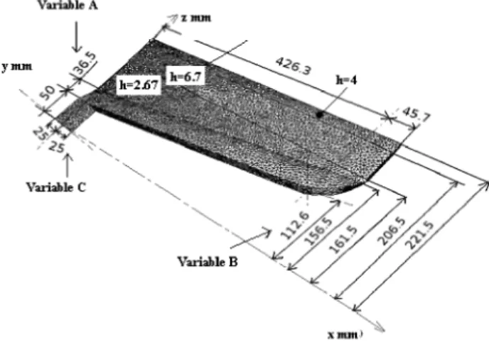
The ultimate goal of this work is to optimize the die channel geometry in a way that a uniform velocity distribution is obtained at the die exit. For this end, we developed an automatic optimization algorithm based on a response surface method together with Kriging interpolation. We used the REM3D® software [12] to compute a 3D flow in extrusion dies. This software takes into account strain rate and temperature dependence. The optimal design procedure is applied to a coat hanger die used to extrude thermoplastic sheets (Figure 1).
Variable A
FIGURE 1. Geometry of the flat die.
THE OPTIMIZATION BENCHMARK
In this paper, the geometry of a flat die is optimized for an Acrylonitrile Butadiene Styrene (ABS, Astalac EPC 10000). The extrusion simulation is carried out using the 3D computation software by finite elements REM3D®. The behaviors laws used in Rem3D® give an expression of the viscosity in function of the shear rate and temperature. The
rheological parameters of the ABS are given in Table 1. Carreau Yasuda/WLF viscosity model is used to characterize the temperature and shear rate dependence [13]. It is written as:
m-1
A flow of 50000 mm3/s was imposed on the entry with a temperature of 240°C, and the temperature of the die is constant and equals to 230°C.
TABLE 1. Rheological parameters.
T]o Pa.s 716.997 Al
m
0.15862 A2[K] CCo 1 Ts[K] Ts Pa 224063 Tref [K] 20.4 101.6 397.7 524.7Design Variables
The design of a flat die is based on the values of various geometrical parameters; the optimization variables (A, B and C) correspond to the geometry of the coat hanger die. The first variable A represents the depth of the channel repartition, the second variable B represents the opening of the channel repartition, the third one C represents the channel thickness (figure 1). During the process of optimization the variables A, B and C vary in a limited field. Each variable has its geometrical limitations which are respectively
30 < ,4 < 110 mm, 50 < B < 140 mm and 5 < C < 45 mm.
During the optimization process, we developed a Matlab® based program which, allows us to treat the CAD and to change the geometry of the die automatically. In the first stage, in order to change the geometry we make a surfaced mesh. Since we know the nodes position, we seek to determine the coordinates of all the nodes (Ni), belonging to both surfaces SI and S2 (figure 2). For this, we use the diffuse approximation [14] with a linear interpolation.
FIGURE 2. Procedure for the change of the geometry.
To change the geometry of the channel repartition we define the new surface (Slk), which corresponds to
the new optimization parameters Ak, Bk, and Ck. After
that, we carry out a change of coordinates for all nodes which belong to the surface SI, so that they will be relocated on to the new Slk surface which represents
the new geometry. For S2 surface, a simple translation of the following nodes is applied there. The same procedure is applied on the other side of the die.
Objective And Constraint Functions
This optimization problem consists in determining an optimal geometry to homogenize the velocity distribution through the die exit, which corresponds to the minimum of the velocity dispersion (E). While preventing that the pressure "pressure loss" increases more than the pressure obtained by the initial geometry. We can also impose a more severe constraint on the pressure; this condition is translated by a constraint function ( g ) .
min J ( O )
Such that g •-P-(a*Po)
( a * P0)
(2) <0
where (J), the normalized objective function, the velocity dispersion (E), is defined as:
f
E
\_N
Z
f\
v
lY\
v
(3) J)where E0 and P0 are respectively the velocity
dispersion and the pressure in the initial die, N is the total number of nodes at the die exit in the middle plane, vi is the velocity at an exit node, and v is the
average exit velocity, is defined as:
1
N(4)
The constraint function ( g ) is selected in a way that it is negative if the pressure is lower than the imposed pressure, if not it will be positive. If a = 1; the pressure should not increase compared to the initial pressure. If a < 1; the pressure must be even lower compared to the initial pressure.
Study of the effects of the variables:
A Taguchi method [3] is used to investigate the effect of the design variables (A, B and C). In the
objective and constraint function we use the response obtained by a central composite design (CDD) [3], which gives 5 levels per variable. The various levels are represented from 1 to 5 respectively giving the values of the minimum to the maximum of each variable. The effects of the various variables are represented on graphs to support the discussion and to lead to the identification of those influencing to minimize the defects.
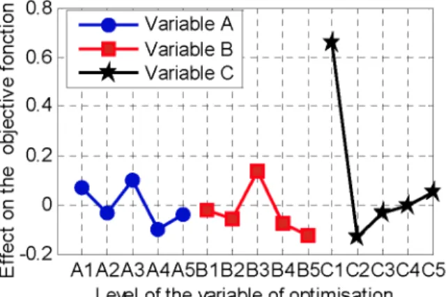
Figure 3, illustrates the average effect of the design variables on the objective function at the various levels. From this figure we can note that the three geometrical variables A, B and C have considerable effects on the objective function, with strongly nonlinear variation according to the various levels. This is more particularly true for the variable A. We notice the variable "C" which represents the thickness of the repartition channel, has a more important effect at level 1 (the minimal thickness of the repartition channel). This effect represents a maximum value, corresponding to a worst exit velocity distribution. At the level 2, the effect represents the minimum value (or best exit velocity distribution). When C is at levels 2 to 5 the effect on the objective function is of same order as the other variables (A and B). It is noticed, from the same figure, that the variables A and B seem having means effects and oscillate compared to the various levels, which implies that a linear or quadratic mathematical model cannot represent effectively the objective function. As for their effects according to the various levels, we note that level 4 of variable A and level 5 of the variable B correspond at the minimum value of the objective function.
0.8 0.6 ~ 0.4
f
O 0.2 •0.2 — ^ — Variable C i i i i i i i - - i— 1 — 1 r — r — r — i -i -i -i -i -i -i -i i i i i i i i i i i i i i i I I A 1 I I I -i -i -i -i -i -i -i I I I T I I I I I I I I I I*k
1 1 1 I 1 I \ l LU A1A2A3A4A5B1B2B3B4B5C1C2C3C4C5 Level of the variable of optimisationFIGURE 3. Effect of the variables on the objective function.
Figure 4, illustrates the average effect of the optimization variables on the constraint function (pressure) at the various levels. It is also noted that the effect of the variable C on level 1 is most important. If the thickness of the repartition channel is minimal (CI) we need more pressure to extrude the plastic. For other
levels of the variable C, we note that the effect is less important, and that the constraint function decreases gradually with the increase thickness of the repartition channel. Concerning the variable A, we note that the effect on the constraint function is average, and the minimum of the pressure corresponds to level 5. This level corresponds to the maximum depth of the repartition channel (figure 1). For this design, the extruded melt undergoes less contracting on the level of the repartition channel and flow out more easily, which can explain the pressure decrease. As for the variable B, we can see that its effect is small on the pressure (constraint), particularly for the levels 1, 2, 4, and 5. For level 3 of variables A and B, the value of the average effect increased because of the taking into account of the maximum value of the effect of the variable C on level 1. ^ 1 5 i 1 1 1 1 1 1 1 1 1 1—j|r—| 1 1 . 5 l l l l l l l V "Q I I I I I I I I 1 C l l l l l l l l I O l l l l l l l l 1 l4— 1 0 — i — ^ 1 — i — i — i — i — ^ ^ — i — V — i — i - £ I I i i i i i i 1 •— I I i i i i i i 1 **— _R i i i i i i i i i i i i i r^ *ft m A1A2A3A4A5B1B2B3B4B5C1C2C3C4C5 Level of the variables of optimisation
FIGURE 4. Effect of the variables on the constraint function.
Optimization procedure
The response surface method consists in the construction of an approximate expression of objective and constraint function starting from a limited number of evaluations of the real function. In order to obtain a good approximation, we used a Kriging interpolation described in next section. In this method, the approximation is computed by using the evaluation points by composite design of experiments.
Once the approximation of the objective function and the constraint function are built for each iteration. Since the successive evaluation of the approximate function does not take much computing time, we use the SQP algorithm to obtain the optimal approximate solution which respects the imposed nonlinear constraints. To avoid the fact of falling into a local optimum, and to respect the imposed nonlinear constraint, we use an automatic procedure which allows the launch of the SQP algorithm starting from each point of our experimental design. We take then
the best approximate solution among those obtained by the various optimizations. Then, another approximate function is built by taking into account the weight function of Gaussian type which allows to slightly change the interpolation and makes the approximation more accurate locally (centred around the best minimum). Next, another minimization is carried out by the SQP algorithm with the initial point which represents the best optimum The iterative procedure stops when the successive points of the approximate function are superposed with a tolerance e=10"6. Finally, another evaluation is carried out to obtain the real response in the optimization iteration.
An adaptive strategy of the search space is applied to allow the location of the global optimum and, then, to readjust the research space by decreasing it by 1/3. A new design of experiment is automatically launched around the optimum. An enrichment of the interpolation is made by recovering responses already calculated, and which are located in the new research space. The iterative procedure stops when the successive points are superposed with a tolerance e=10-3.
Kriging interpolation
Kriging (27, 28), is an elegant and general interpolation method. Its origin goes up to Krige at the beginning of the 50th, it was proved to be a very powerful interpolation technique. The Kriging, makes it possible to present the complexes function effectively (curved, surfaces...). This method is applied in our work to represent the response surface in an explicit form, according to the variables of optimization.
J(x) = pT(x)a + Z(x) (5)
with, p(x) = [p1(x), ..., pm(x)f, where m
denotes the number of the basis function in regression model, a = fav ..., am] is the coefficient
vector the, x is the design variables, J(x) is the unknown objective or constraint interpolate function, and Z(x) is the random fluctuation. The term
p (x)a in Eq. (5) indicates a global model of the design space, which is similar to the polynomial model in a Moving Least Squares (MLS) approximation. The second part in Eq. (5) is a correction of the global model. It is used to model the deviation from p (x) a so that the whole model interpolates response data from the function
The construction of a Kriging model can be explained as follows:
The output responses from the function are given as:
F(x) = {f
1(x\f
2(x\-fA*)} (6)
From these outputs the unknown parameters a can be estimated:
a = (P
1R-'PpP
1R
lF
(7)Where P is a vector including the value of p(x) evaluated at each of the design variables and R is the correlation matrix, which is composed of the correlation function evaluated at each possible combination of the points of design:
R
^ ( * i ,xi ) • " ^ ( * i ,xJi?(x
n,
X l) ... R(x
n,x
n)
R
'j4
(8) (9) The second part in Eq. (5) is in fact an interpolation of the residuals of the regression model/? (x)a . Thus, all response data will be exactly predicted; is given as:Z(x) = rT(x)P (10)
Where rT(x)= {R(x,x1),---,R(x,xn)}
The parameters /? are defined as fallow:
P = Rl(F-Pa) (11)
R E S U L T A N D D I S C U S S I O N
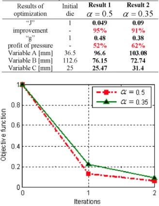
A representative convergence history during an optimization process on the objective functions (J) is represented in figure 5. Two curves of results of the convergence of optimization are presented:
Results 1: A constraint on the pressure is imposed for which the pressure in the optimal die must be lower or equals 0.5*P0 {a = 0.5).
Results 2: The constraint imposed on the pressure is more severe. The pressure in the optimal geometry must be lower or equals 0.35*P0 (CC = 0.35).
Our algorithm of optimization clearly showed its capacity to obtain an optimal solution with a very fast
convergence. The optimal solution is obtained in two iterations for both cases. The objective function is then reduced to: 95 % of its initial value, for the first result
a = 0.5 . And 91% of its initial value, for the second result a = 0.5
TABLE 2. Summary of the results. Results of optimization Initial die Result 1 or = 0.5 Result 2 or = 0.35 "J" improvement "g" profit of pressure Variable A [mm] Variable B [mm] Variable C [mm] 1 -1 -36.5 112.6 25 0.049 95% 0.48 52% 96.6 76.15 25.47 0.09 91% 0.38 62% 103.08 72.74 31.4 0 1 2 Iterations
FIGURE 5. Convergence history during an optimization process on the objective functions.
We notice that the objective function for both results has strongly decreased in the first iteration, because of the precision of the Kriging interpolation. Nevertheless, to respect the constraint while ensuring a homogeneous distribution of velocity, we observe that result 1 offer the best minimum in the first and second iteration, because of the less severe constraint on the pressure compared to results 2.
We have represented the relative velocity dispersion obtained in the initial geometry and after optimization, for both results in figure 6. We see that the objective function obtained by imposing a severe constraint on the pressure (a = 0.35) is slightly higher of the objective function obtained with a less severe constraint ( a = 0.5).
S- 60 •E 50 Initial die Optimal die a = 0.5 Optimal die ct= 0.35 jjjdPat 100 200 300
Width of half die fmml
FIGURE 6. Velocity dispersion with initial and optimal die.
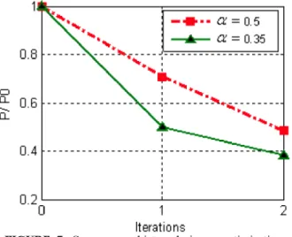
The constraint on the pressure is represented on figure 7, in a form of (P/PO) for both results. We see that the constraint function is weaker with a more severe constraint ( a = 0 . 3 5 ) .
o
0 1 2 Iterations
FIGURE 7. Convergence history during an optimization run of the Constraint functions.
CONCLUSION
The applied method of optimization with the various strategies allowed us to obtain an optimal geometry in two iterations with a very satisfactory computing time for E.F calculation of the flow in three dimensions. The optimal die gives a good exit velocity distribution while minimizing the pressure for the same flow. A qualitative comparison enables us to note that we were able to obtain with the optimal geometry a 9 5 % profit of homogeneity compared to the initial geometry with a decrease of pressure of 52% (results obtained with a less severe constraint on the pressure). The use of the different constraints on the pressure allowed us to
compare the various results obtained after optimization. The results are obtained at the second iteration. The algorithm of optimization clearly showed its robustness and its capacity to obtain an optimal solution with a very fast convergence. Total CPU time is of 3 days and 16 hours on a machine Pentium IV, 3 GHz, 1 Go RAM.
R E F E R E N C E S
1. Y. Wang, "The flow distribution of molten polymers in slit dies and coat hanger die through three-dimensional finite element analysis," In Polymer Engineering and
Science, 1991, pp. 204-212.
2. P. Hurez, P. A. Tanguy, D. Blouin, "A New Design procedure for profile die," In: Polymer Engineering and
Science, Vol 36, No 5, 1996, pp. 626-635.
3. D.C. Montgomery, "Design and analysis of experiments," John wiley & Sons, INC, USA, 2005. 4. C. Chen, P. Jen, F. S. Lai, "Optimization of the
Coathanger manifold via computer simulation and orthogonal array method," In Polymer Engineering and
Science, 1997, pp. 188-196.
5. Y. W. Yu, T. J. Liu, "A simple numerical approach for the optimal design of an extrusion die," In: Journal of Polymer Research, 1998, pp. 1-7.
6. Y. Xiaorong, S. Changyu, L. Chuntai, W. Lixia, "Optimal design for polymer sheeting dies," In Chinese
Journal of Computational Mechanics, 2004, pp. 253-256.
7. D.E. Smith, D.A. Tortorelliav, CL. Tucker, "Optimal design for polymer extrusion. Part I: Sensitivity analysis for nonlinear steady-state systems," Comput. Methods
Appl. Meek Engrg. 1998, pp. 283-302.
8. D.E. Smith, D.A. Tortorelliav, CL. Tucker, "Optimal design for polymer extrusion. Part II: Sensitivity analysis for weakly-coupled nonlinear steady-state systems," in
Comput. Methods Appl. Mech. Engrg. 1998, pp.303-323. 9. D.E. Smith, "An optimisation-based approach to
compute sheeting die designs for multiple operating conditions," In: Annual Technical Conference, 2003, pp. 315-319.
10. W. Michaeli, S. Kaul, T. Wolff, "Computer aided optimisation of extrusion dies," In: Journal of Polymer
Enginering, 2001, pp. 225-237.
11. Y. Sun, M. Gupta, "Optimization of a flat die geometry,"
InAnnual Technical Conference, 2004, pp. 3307-3311. 12. L. Silva, "Viscoelastic Compressible Flow and
Applications in 3D Injection Molding Simulation," these de doctorat, CEMEF, 2004.
13. G. Balasubrahman, D. Kazmer, "Thermal control of melt flow in cylindrical geometries," In: Annual Technical Conference, 2003, pp. 387-391.
14. N. Lebaal, S. Puissant, F. M. Schmidt, "Rheological parameters identification using in-situ experimental data of a flat die extrusion," In Journal of Materials
Processing Technology, 2005, pp.1524-1529.