HAL Id: hal-00620874
https://hal.archives-ouvertes.fr/hal-00620874
Submitted on 8 Sep 2011
HAL is a multi-disciplinary open access
archive for the deposit and dissemination of
sci-entific research documents, whether they are
pub-lished or not. The documents may come from
teaching and research institutions in France or
abroad, or from public or private research centers.
L’archive ouverte pluridisciplinaire HAL, est
destinée au dépôt et à la diffusion de documents
scientifiques de niveau recherche, publiés ou non,
émanant des établissements d’enseignement et de
recherche français ou étrangers, des laboratoires
publics ou privés.
Handling uncertainty in production activity control
using proactive simulation
Olivier Cardin, Pierre Castagna
To cite this version:
Olivier Cardin, Pierre Castagna. Handling uncertainty in production activity control using proactive
simulation. 12th IFAC Symposium on Information Control Problems in Manufacturing, INCOM 2006,
2006, Saint-Etienne, France. pp.579-584. �hal-00620874�
HANDLING UNCERTAINTY IN PRODUCTION ACTIVITY CONTROL USING PROACTIVE SIMULATION
Olivier CARDIN Pierre CASTAGNA
Institut de Recherches en Communication et Cybernétique de Nantes 1 rue de la Noë
44321, Nantes FRANCE
Abstract: Simulation is a powerful tool used for a long time as a help to production systems conception. Proactive simulation is a new approach, enabling a precious help to these systems control. In this paper is presented a control architecture enabling the use of this tool, and the obstacles to an optimised development. Copyright © 2006 IFAC
Keywords: Simulation, Scheduling, Uncertainty, Production Control, Manufacturing Systems, Proactive, Real-time.
1. INTRODUCTION
In today's complex manufacturing setting, with multiple lines of products, each requiring many different steps and machines for completion, the decision maker for the manufacturing plant must find a way to successfully manage resources in order to produce products in the most efficient way possible. The decision maker needs to design a production schedule that promotes on-time delivery, and minimizes objectives such as the flow time of a product. Real-word planning and scheduling problems are generally complex, constrained and multi-objective in nature.
For short-term production scheduling, alternative methodologies and problem statements with different considerations have been proposed in the literature. Most of these works rely on mathematical programming approaches based on discrete or continuous-time representations. Although these rigorous methods are able to guarantee the optimality of the solution, their applicability is currently restricted to quite small cases due to the inherent combinatorial nature of scheduling problems. To overcome this limitation, a wide variety of heuristic and rule-based procedures have been developed aiming at providing good schedules to large-scale
problems in a reasonable time. Recently, there has been a high research interest in evolutionary, meta-heuristic and soft computing approaches for solving scheduling problems.
The problem of most of these scheduling solutions in the literature is they need a perfect knowledge of all the parameters involved in the computation of the scheduling.
A lot of the production systems, taking into account testing operations for example, cannot fit in this category. Indeed, as soon as the recipes of the products can be modified along the production, the result of the scheduling operation is not up-to-date anymore and thus another scheduling operation should be run. Due to the frequency of this event, and due to the complexity of the operation, another solution has to be defined.
Moreover, due to the growing complexity of the production systems, the decisional system (Le Moigne, 1990; Lenclud, 1993), which runs the production system, has to take a lot of decisions along the production. To be able to take satisfying decisions, two conditions have to be respected. First, the decisional system must have at his disposal reliable, complete and frequently updated data, giving him a satisfying view of the system. The proposition in this paper is to add a real-time
simulation in the control architecture. This simulation plays the role of an observer, rebuilding, thanks to the partial data retrieved from the system, all the data needed to take a decision.
Secondly, the decisional system must be able to evaluate the impact of the different options available. As a matter of fact, a decision model has to be made. This model must be at the same time accurate, i.e. the forecasts must be sharp and correspond as much as possible to the system, and quick. Indeed, facing a given situation, the decisional system has a short time to react and make a decision.
The complexity of the production systems makes that no satisfying analytical model exists: this paper presents the use of a proactive simulation module as decision model.
First, the concept of a real-time simulation observer is developed. Then, the proactive simulation module is described before presenting an application of these principles in last part.
2. OBSERVING A SYSTEM BY REAL-TIME SIMULATION
Traditionally, simulation is used as a prediction tool. As a matter of fact, time in simulation runs as fast as possible to try and reduce the simulation time. To achieve this, simulation tools have an engine base on events. The simulator builds an events calendar, ordered list of all the events that can be dated, chronologically sorted. Then it executes the first event of the list and rebuilds the calendar, which has been modified by the event. This working is very fast, as the simulator goes from event date to event date, without considering dates where nothing is supposed to happen.
In a real-time simulation, the engine is very different. Indeed, the simulated time is adjusted with the real time (synchronously with the CPU clock).
The main application of real-time simulation is the development of simulation models meant to verify the behaviour of real-time software (Schludermann et al. 2000, Cofer and Rangarajan, 2003).
In this paper, another utilization of real-time simulation is presented. The decision maker needs to have, in order to be able to make a choice, a complete description of the actual production system state. To do that, a Manufacturing Execution System (MES) is used.
"A Manufacturing Execution System (MES) is a dynamic information system that drives effective execution of manufacturing operations. Using current and accurate data, MES guides, triggers, and reports on plant activities as events occur from point of order release into manufacturing to point of product delivery into finished goods" according to Manufacturing Enterprise Solutions Association International (MESA). MES is the central source for current information on the manufacturing floor. These data are delivered by means of sensors to be placed on the production floor. The problem is that the MES is not able to give us all the state of the
system, at any time, because of the limited number of sensors. So, a real-time simulator will be used as an observer of the physical system.
The application will reproduce the behaviour of the production system. Thus, the whole state of the system will be known through the state of the simulator.
Of course, it will be necessary to insure equivalence between the evolution of the model and the evolution of the system. To achieve this, the simulator will automatically track the physical system thanks to the data coming from the system through the MES. The MES knows the state of the physical system through the state change of a set of sensors. The link between the MES and the simulator enables the achievement of a tracking each time the MES detects a new event.
Two possibilities may appear. On the first one, the simulator is ahead of the physical system. In this case, the simulator has to wait the event coming from the MES. It means the simulation model must be aware of all the situations where a synchronisation has to be done. The model evolves until reaching such a situation, and locally waits for this data. The evolution of this part of the model will only keep going when the data will be sent by the MES, whereas the rest of the model keeps on going normally.
On the second possibility, the data come from the MES before the model reaches the synchronisation point. At this point, a local time acceleration in order to bring the simulator in a state conformed to the physical system is used.
As an illustration, let’s take a conveyor and two sensors s1 and s2 (Fig. 1).
On the simulation, a transporter (1) is in front of sensor s1, whereas the real one is not arrived yet. This is the first case previously described. The simulator will then block the transporter in that position until the real sensor s1 detects the real transporter (1).
On the opposite, the real transporter (2) is in front of sensor s2 whereas the simulator displays (2) far before sensor s2. The real system is ahead the simulator. The tracking will instantaneously put simulated transporter (2) in position (2b).
Obviously, each time the system is known by the MES, there will be no difference between the behaviour of the simulation and the behaviour of the physical system. However, between the two sensors, the position of the transporters is totally unknown.
s1 Physical system Simulated system
(1)
s2 s1 s2 (1) (2) (2b) (2)The simulation is then used to know this position by simulating the moving of the transporters.
Let’s note that, because of the use of two interlocked simulations, this work is set in the concept of reflective simulation (Kindler et al., 2001).
3. USING THE PROACTIVE SIMULATION Flow simulation is widely used to study production system. For a long time, it was only used in the conception or re-conception phase of the production system. In Castagna et al. (2001), it was proposed to use simulation as a Decision Helping Tool, with the example of a production unit of the aeronautic industry.
In Pujo et al. (2004), simulation was used inside the Production Activity Control of a unit organised with KANBAN. It is shown that, thanks to proactive simulation, “the production manager […] can lean on forecasts, simulated from structural data of the workshop synoptic, and a model representing the running production considering the actual state of the workshop, permanently updated with the events, planned or contingent, which happen”.
To develop proactive simulation on commercial software, two main problems may appear: the duration of the simulation and its initialisation.
3.1. The duration of a proactive simulation
Frequently, simulation of an industrial problem is several hours long. In a conception phase, this has no impact on the pertinence of its use. For a proactive simulation, this duration is totally unacceptable. The decisional system has a very short time to make its decision, and the simulation is included in this time as a part of the data retrieval.
Let’s consider:
DT Total duration available for the
decisional system to make its decision, DC Duration needed for the retrieval of
the data needed for the simulation DS Total duration of the simulation,
DD Decision-taking time, simulation
results being known.
The following relationship must be respected. DC +DS + DD ≤ DT
In the DS time, several simulations can be run, each
one corresponding to a different scenario to be tested. In each scenario, the decision maker applies a different decision, which obviously leads to a different events series. If the model is deterministic, and the run of a simulation is Du long, then DS = N
Du will be needed to test N possible scenario.
Furthermore, if the model takes into account stochastic events and that M replications are necessary to increase the confidence interval, then the duration of the simulations will be:
DS = N M Du
All along the model building, a particular care will be brought to the running duration. Fortunately, the simulation horizon needed for decision taking is frequently relatively short.
3.2. The initialisation of a proactive simulation
Most of the simulation tools consider the production system empty at initial state. Thus, there is a time at the beginning of each replication devoted to a progressive loading of the production system. If this is not representative of the working of the system, it must be removed.
In a proactive simulation, the initial state must be the exact one of the production system. The model has to be brought to this non-empty state starting from an empty system and following a track that will lead it to the correct initial state. This may quickly become very tricky. The idea in this work is to configure the simulator directly in the correct initial state.
But, the data retrieval is still a problem. This retrieval has to be quick to decrease DC. As seen previously,
the MES does not have all the data required by the simulator for its initialisation. For example, the model needs the exact position of all the transporters all along the system.
A communication link is thus settled with the observer (i.e. the real-time simulation) in order to complete the data brought by the MES: to the production data provided by the MES are added simulated data provided by the observer.
In the next section these concepts are developed on an assembly line.
4. APPLICATION ON A COMPLEX MANUFACTURING SYSTEM
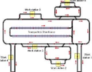
The assembly line was built for educational and research purposes by the Institut Universitaire de Technologie of Nantes (Fig. 2). This job shop production system is made of six workstations. The goods are transported with pallets, which move on unidirectional conveyors. The pallets will be called transporters”.
Fig. 2. The job-shop production system
A transporter storehouse (an accumulation conveyor) enables the storage of the free transporters. The working of the line is based on the concept of “Intelligent Product” (Wong et al., 2002). The 42 transporters are equipped with smart tags. These tags enable an Auto-Identification when in front of a tag reader. The data contained on the tag are part of the decision making process. As lots of decisions are made at a local scale, the global behaviour of the line is hard to model.
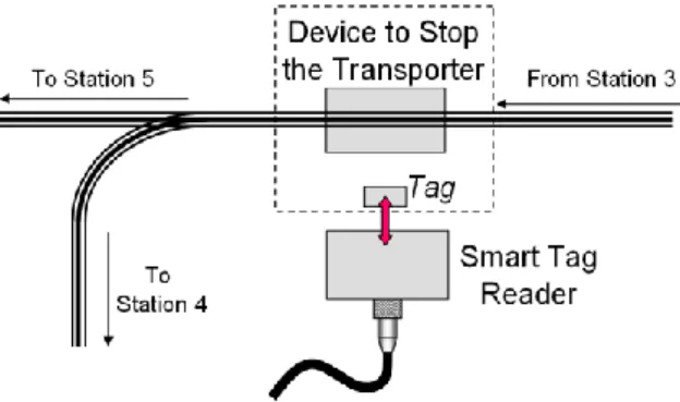
Indeed, if, for example, the product needs to go on stations 4, 6 and 3 (in this order) to perform the operations required, the transporter moves on the main loop until reaching the entrance of the work station 4 (Fig. 3).
Fig. 3. The job-shop production system At this point, a local decision is taken, making the transporter enter (or not) the station. This decision depends on a lot of parameters (number of transporters in the station batch, breakdowns of the station etc.).
Furthermore, the recipe of the product is an ordered list of operations, not a list of stations. As a matter of fact, it is frequent that two stations perform the same operation. Thus, the entrance rule may become a lot more complicated if, for example, the pilot chooses to let one transporter out of two come in to balance the load of the stations.
Similarly, stations 2 and 6 may not have a FIFO priority rule. Indeed, the configuration of the batches makes it possible to use dynamic scheduling methods as list algorithms (Kim, 1995) or more complicated rules as “Clear a Fraction” for example (Kumar and Seidman, 1990).
Finally, it is possible to take into account test operations. If the test is passed, the product goes on, but if it is not, the recipe of the product is modified to either treat the defective goods or rework it. All these properties make this example particularly adapted to the subject of this work, as the line is almost impossible to model analytically.
5. THE CONTROL ARCHITECTURE The Human Machine Interface in the control architecture is made with a supervisor, part of the Manufacturing Execution System with a database. An OPC server is settled as an intermediate between
the Programmable Logic Controllers and the MES (Fig. 4).
OPC (OLE for Process Control) is a communication standard based on OLE/COM technology (Object Linking and Embedding/Component Object Model), which constitutes a unified mean of data exchanges between software. It offers a great interoperability (read/write) between the industrial equipments (PLC, sensors etc.), all the monitoring/control/supervision software and the office management software. It also defines standard objects, methods and properties based on COM concept to enable real-time data servers (as PLC) to transfer the data to client OPC applications. The server handles the refresh of the data. Its rate may be different according to the technology, in particular the communication protocols.
Fig. 4. The control system
In this case, the OPC server is used as a common platform of communication between any application and the PLC. This enables the insertion of as many elements in the architecture as wanted without disturbing the other ones.
Indeed, both of the simulation applications have to be linked to this architecture. As the system must be able to run without the simulation help, these applications are aggregated in a single module (Fig. 4).
The module may be set for two different workings: automatic or manual. Next sections will describe these two modes.
5.1. Manual working
To illustrate this working, let’s take the example of a major failure of station 1 of the assembly line. The pilot expertise says it is necessary to re-organize the workshop. All the five operations performed on the station have to be reassigned to other stations. At this point, the use of proactive simulation can be broken down into 7 steps:
1. The pilot launches the simulation module (Present Time = PT). The actual state of the
system is saved.
2. He sets the total decision time DT and the
3. He enters one of the new possible sets of operations performed on the stations corresponding to one of the possible scenario. 4. The simulation is launched. It is initialised from
the state saved in step 1. The production keeps going on without any change until simulated time PT+DT is reached, and then the changes are
made on the operations.
5. Once the simulation is over, either a new replication of the same scenario is launched or a new scenario is tested (step 3).
6. All the results are saved in a separate file. The pilot can make a decision, based on the analysis of all these results.
7. At real time PT+DT, the decision is applied on
the production system.
The pilot can analyse the results with the same methods as those used in the usual post-production analysis. Indeed, the simulation gives the same kind of results than the real production, which makes this analysis easier.
Obviously, this working is very flexible and enables lots of possibilities. The crucial point here is once more the time question, since a lot of replications could be necessary (several hundreds in some cases). Hopefully, the poor programming complexity allows a fast evolution of the proactive simulation.
5.2. Automatic working
In automatic working, the simulation must be transparent to the user. As two different simulations cannot be run on the same CPU, a separate dedicated computer may be useful.
As soon as the automatic simulation module is turned on, the behaviour of the line changes. An application of this feature is described in Cardin and Castagna (2005), enabling the use of the “Clear a Fraction” rule with a proactive sight to decrease the number of settings.
In this mode, the decision of performing a simulation is taken without any action of the pilot. In a given configuration, a local decision module asks for a simulation result. The information is transmitted to the simulation module through the OPC server. Eight steps can describe the working of the module:
1. When the event is generated (Present Time=PT), the actual state of the system is
saved.
2. The total decision time DT and the simulation
horizon are automatically calculated by the module.
3. The model corresponding to the question asked is launched (each different type of question has an own model).
4. The parameters of the simulation are set. 5. The simulation is launched. It is initialised from
the state saved in step 1. The production keeps going on without any change until simulated time PT+DT is reached, and then the changes are
made.
6. Once the simulation is over, either a new replication of the same scenario is launched or a new scenario is tested (step 3).
7. The module analyse the results (the decisions procedure are decided during the building of the architecture and may be different in each application).
8. At real time PT+DT, a VBA procedure directly
modifies the affected PLC variables thanks to the OPC server.
Obviously, this working is not flexible, as everything must be programmed before its use on the production system, but the absence of interaction with the human operator makes the execution time (and thus the Decision Time) a lot shorter. As a matter of fact, this is meant to be applied to decisions that have to be made in a few seconds.
Indeed, the decisions can be made on criteria as much complicated as wanted, if the decision protocol is correctly defined and based on a good expertise.
5.3. Results
On a temporal point of view, some tests were made to evaluate the time needed for each step to be completed in automatic working. The same tests cannot be significant in manual working as it mostly depends on the time the pilot needs to make his decision, which fluctuates widely according to the problem posed.
If steps 1 and 2 (backup of the actual state), 3, 4 and 5 (initialisation of the simulation) all together are 1 second long (DC), step 6 corresponding to the
simulation itself is about 3 seconds long (DS). As the
analysis of the results and the time needed to apply the decision is about 1 second long (DD), a whole
simulation lasts less than 5 seconds (DT). This result
is fully satisfying as it is compatible with an online use. Of course, this solution may be adapted if the production rate is too high.
Then, tests were made to estimate the impact on the production of the solution presented here. The results are shown on Table 1.
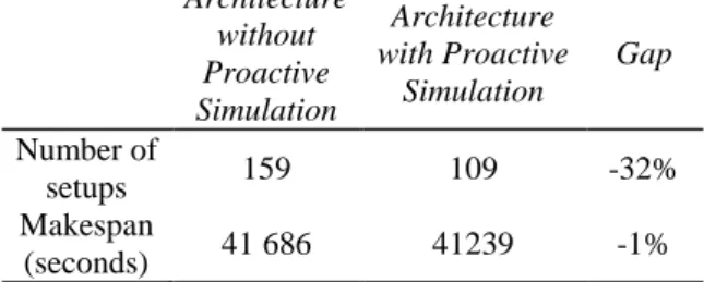
Table 1 Comparison between workings with and without proactive simulation
Architecture without Proactive Simulation Architecture with Proactive Simulation Gap Number of setups 159 109 -32% Makespan (seconds) 41 686 41239 -1% The problematic of this test was to decrease the number of setups of workstation 6. Indeed, this station represents a painting station, and changing the operation means changing the trajectories of the robot and the colour of the painting. As a matter of fact, paint is lost at each setup. The Clear-a-Fraction rule was implemented in this aim, but better
performances are required. The results show a fall-off of the number of setups thanks to Proactive Simulation (-32%): this result confirms the impact of the new architecture on the real system.
Furthermore, the makespan remains globally constant. As proactive simulation is implemented on a single work station (work station 6), its productivity is modified (in this case, it is increased). But the previous station in the recipe is not able to supply enough products to work station 6. Similarly, the next station in the recipe is not able to deal with all the products coming from station 6, thus it slows the production down. This is why the gap between the production with and without simulation is so small (about 1%).
6. CONCLUSION
This study shows how much simulation can be included in a proactive approach of the Production Activity Control of a manufacturing system with uncertainties. It can be as well used for global scheduling of the workshop activity, or on a very local point of view, improve the behaviour of the system.
As a matter of fact, proactive simulation is:
— Either a data complement given to the pilot of the line in order to be able to take the best decision
— or a possibility to control the line taking into account what is going to happen next.
All the elements needed to use proactive simulation are meant to be aggregated in a single module (containing several computers linked by an Ethernet network), which can be plugged in or out without stopping the system working.
In this module, two main elements may appear: the real-time simulation and the proactive simulation. The real-time simulation model is close to a classical simulation model (except for the communications with the other elements of the architecture), and thus this is possible for an operator well versed in flow simulation to build it.
Each time a new type of proactive simulation is required, a new model has to be made. This model is only a modification of the original model, but a large set of strict rules has to be respected. As a matter of fact, an expert in simulation is required at the time being. A future development of this work is planned about the definition of libraries useful in the proactive simulation models building to make this easier.
Another land to explore is the definition of the decisional system. Indeed, in an automatic working, it takes several decisions autonomously. Thus it needs a decision algorithm based on the expertise of the pilot of the line. This algorithm still needs to be elaborated.
REFERENCES
Cardin O., P. Castagna (2005), Defining A Command
Architecture Enabling Proactive Simulations On A Complex Manufacturing System, in
Proceedings of the I3M Conceptual Modeling and Simulation Conference CMS’2005, Marseille, France.
Castagna P., N. Mebarki, R. Gauduel, (2001), Apport
de la simulation comme outil d’aide au pilotage des systèmes de production - exemples d’application, in Proceedings of the 3e
Conférence Francophone de MOdélisation et SIMulation MOSIM’01, Troyes, France. Cofer Darren D. and Rangarajan M., (2003).
Event-triggered environment for verification of real-time system, in Proceedings of the 2003 Winter
Simulation Conference, ed. S.Chick, P. J. Sánchez, D. Ferrin, and D. J. Morrice,. Piscataway, New Jersey: Institute of Electrical and Electronics Engineers. p. 915-922.
Kim Y-D (1995), A backward approach in list scheduling algorithms for multi-machine tardiness problems, Computers and operations
research, Volume 22, Issue 3, March 1995,
Pages 307-319
Kindler E., I. Krivy and A. Tanguy, (2001). Tentative
de simulation réflective des systèmes de production et logistiques, in Proceedings of the
3e Conférence Francophone de MOdélisation et SIMulation MOSIM’01, Troyes, France, Volume 1, pp. 427-434.
Kumar P. R. and I. T Seidman., (1990) Dynamic
Instabilities and Stabilization Methods in Distributed Real Time Scheduling of Manufacturing Systems, IEEE Trans. on A.C.
35(3), pp. 289-298.
Le Moigne J.-L., (1990), La modélisation des
systèmes complexes, Editions Dunod.
Lenclud T., (1993), Contribution à la conception
d'un système intégré de simulation des systèmes de production, Thèse de doctorat, Université de
Valenciennes et du Hainaut-Cambresis, France. Pujo P., M. Pedetti and F. Ounnar, (2004), Pilotage
proactif des lignes de production kanban par modélisation DEVS et simulation temps réel, in
Proceedings of the 5e Conférence Francophone de MOdélisation et SIMulation, MOSIM'04, Nantes, France, p.593-600.
Schludermann H., Kirchmair T. and Vorderwinkler M., (2000), Soft-commissioning:
Hardware-in-the-loop based verification of controller software, in Proceedings of the 2000 Winter
Simulation Conference. p.893-899.
Wong CY, D McFarlane, A Zaharudin and V Agarawal, (2002), The Intelligent Product
Driven Supply Chain, in Proceedings of IEEE