Restoration of ultrasonic images using non-linear system identification and deconvolution

Official URL

DOI :

https://doi.org/10.1109/ISBI.2018.8363778

Any correspondence concerning this service should be sent

to the repository administrator:

[email protected]

This is an author’s version published in:

http://oatao.univ-toulouse.fr/24698

Open Archive Toulouse Archive Ouverte

OATAO is an open access repository that collects the work of Toulouse

researchers and makes it freely available over the web where possible

To cite this version: Hourani, Mohamad and Basarab, Adrian and

Kouamé, Denis and Girault, Jean-Marc and Tourneret, Jean-Yves

Restoration of ultrasonic images using non-linear system identification and

deconvolution.

(2018) In: 15th IEEE International Symposium on

Biomedical Imaging: From Nano to Macro (ISBI 2018), 4 April 2018 - 7

April 2018 (Washington DC, United States).

RESTORATION OF ULTRASONIC IMAGES USING NON-LINEAR SYSTEM

IDENTIFICATION AND DECONVOLUTION

Mohamad Hourani

, Adrian Basarab

, Denis Kouamé

, Jean-Marc Girault

, Jean-Yves Tourneret

2_{University of Toulouse, IRIT, CNRS UMR 5505, Université Paul Sabatier, Toulouse, France}

3_{Department of Medical Biophysics and Imaging, Signal-Imaging Group, François-Rabelais University of Tours, France}

{mohamad.hourani,adrian.basarab, denis.kouame}@irit.fr, {jean-yves.tourneret}@enseeiht.fr, {jmgirault@}@univ-tours.fr,

ABSTRACT

This paper studies a new ultrasound image restoration method based on a non-linear forward model. A Hammerstein polynomial-based non-linear image formation model is considered to identify the system impulse response in baseband and around the second har-monic. The identification process is followed by a joint deconvolu-tion technique minimizing an appropriate cost funcdeconvolu-tion. This cost function is constructed from two data fidelity terms exploiting the linear and non-linear model components, penalized by an additive ℓ1-norm regularization enforcing sparsity of the solution. An

alter-nating optimization approach is considered to minimize the penal-ized cost function, allowing the tissue reflectivity function to be esti-mated. Results on synthetic ultrasound images are finally presented to evaluate the algorithm performance.

Index Terms— non-linear model, system identification, har-monic ultrasonic imaging, optimization, ADMM, polynomial Ham-merstein model, deconvolution.

1. INTRODUCTION

Ultrasound (US) imaging is an effective, low cost, harmless and non-invasive medical imaging modality [1]. It is therefore widely used for clinical diagnosis (mainly for soft tissue applications related to cardiovascular and various cancers), blood flow velocity assessment and obstetrics. However, because of instrumentation constraints, US images suffer from a relatively low contrast, reduced spatial reso-lution and signal-to-noise ratio. Specifically, US images are con-taminated by an intrinsic noise called speckle, which appears as a granular texture in the image. It is well known that speckle deeply reduces the general image quality in terms of contrast and resolu-tion and increases the margin of inaccuracy in diagnostic analysis. Improving US image quality through post-processing image restora-tion techniques is therefore an important research area. Note that instrumentation approaches or pre-processing methods such as non-conventional beamformers have been also explored in the context of US [2]. In addition to the aforementioned limitations of ultra-sound imaging, the propagation of ultraultra-sound in many tissues is non-linear. Consequently, the resulting signals are combination of linear and non-linear components. This paper explores a deconvo-lution approach based on a new non-linear image formation model. This model is able to express different degrees of nonlinearity gen-erated by the tissues themselves or by ultrasound contrast agents [3]. Most of the existing US image restoration methods use the first or-der Born approximation and consequently assume that the tissue re-flectivity function (TRF) is related to the US radiofrequency (RF) image through a 2D convolution with the system point spread

func-tion (PSF) [4–7]. However, this forward model widely explored in the literature does not exploit the non-linear relationships that can exist between the unknown TRF and the observed image. We pro-pose herein a new image restoration method originating from a study of non-linear ultrasonic wave propagation in a medium [1]. More specifically, we investigate a different perspective for US image de-convolution, i.e., we estimate the TRF by eliminating the contribu-tion of the system excitacontribu-tion and the PSF using a non-linear image formation model. The non-linearity considered in this work results from a polynomial Hammerstein model allowing PSF identification. More specifically, we focus in this paper on identification methods for a generalized polynomial Hammerstein model based on an expo-nential swept-sine input signal, allowing one-path estimation of the unknown linear filters. This identification method, originally pro-posed by Farina et al. [8] and further explored by Novak et al. [9] and Rebillat et al. [10], allows the TRF of the explored medium to be estimated. The proposed estimation method optimizes a joint cost function based on both the linear and non-linear components of the model using the alternating direction method of multipliers (ADMM). The remainder of the paper is organized as follows. Sec-tion 2 describes the non-linear model considered in this study and the corresponding parameter identification approach. Section 3 in-troduces the proposed image restoration framework and the corre-sponding ADMM algorithm. Simulation results are reported in Sec-tion 4 before concluding the paper.

2. PROBLEM STATEMENT 2.1. Nonlinear Model

The use of non-linear models in US imaging is mainly motivated by the strong non-linearities that are caused by the interaction be-tween the US waves and some particular tissues. Therefore, several non-linear models can be found in the literature for non-linear US simulation [11] or for the analysis of US images, such as Volterra se-ries [12], neural networks [13] or Hammerstein models [14]. These models depend on unknown parameters or kernels to be estimated from the data. In this paper, we use the non-parametric general-ized polynomial Hammerstein model due to its generic structure: this non-linear system can be represented byN parallel branches, each branch being composed of a non-linear static polynomial ele-ment followed by a linear impulse response block. All branches have a common excitation x(t). The relationship between the input x(t) and the output y(t) is given hereafter

y(t) =

N



n=1

where∗ denotes convolution and gn(t) is the impulse response of

thenth_{branch. In this work, g}

n(t) includes both the system PSF

at the corresponding ordern and the TRF representing the true im-aged field topography. In this work, the number of system branches is limited to two, i.e., a linear component resulting from the linear image formation model and a second one associated with the first harmonic resulting from the non-linear interactions in the field. For N = 2 and taking into account the transducer’s limited bandwidth (both in reception and emission), the model in (1) can be reformu-lated as

y(t) = x(t) ∗ g1(t) + x2(t) ∗ g2(t) + n(t) (2)

where g1(t) and g2(t) are the system impulse response in baseband

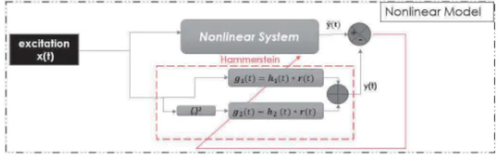
and arround the first harmonic and n(t) is an additive white Gaus-sian noise (AWGN). A schematic representation of the model in (2) is shown in Fig. 1.

Fig. 1. Schematic representation of the non-linear generalized polynomial Hammerstein model considered in this work.

2.2. System identification

This work assumes that the excitation x(t) is known such that the identification process only concerns the estimation of g1(t) and

g2(t) from y(t) and x(t). The estimation of the model impulse

responses in (2) has been already explored in the literature and de-pends on the nature of the excitation x(t) (see, e.g, [15] for a sine wave excitation or [16] for a random excitation). Assuming the model input x(t) is known and observing the output signal y(t), the identification approach used herein is based on the convolution between the output of the non-linear system and the inverse filter associated with the input. This work focuses on a swept-sine signal x(t). In this case, the identification process has an analytical solu-tion obtained from the instantaneous frequency step parametrizasolu-tion during one time step [9,10,17]. The analytical inverse filter, denoted byx(t), is a matched filter, i.e., the time-reversed signal associated! with the input x(t). As explained in [9], the convolution between the system output y(t) and the estimated input !x(t) allows the excitation x(t) to be removed from (2). Indeed, the result of this so-called "non-linear convolution" can be written

z(t) = y(t) ∗ !x(t) =

2



n=1

gn(t + ∆tn) (3)

where∆tnis the temporal gap between the non-linear impulse

re-sponse (IR) (n = 2) and the fundamental IR (n = 1). One of the main advantages of this convolution is that it allows the system IRs to be estimated in one path, i.e., the result of the convolution is a set of IRs separated in time with a delay∆tn. This separation allows

the IRs of the two branches g1(t) and g2(t) to be estimated after

time windowing. The two estimated IRs are then used in the next section for estimating the TRF of the US image.

3. ULTRASOUND IMAGE DECONVOLUTION The non-linear model and its identification presented in Section 2 have been included in a US image deconvolution framework

allow-ing the system excitation and the PSF to be separated from the TRF. The proposed TRF restoration method follows two steps. First, the excitation is eliminated through the identification presented in Sec-tion 2.2. In a second step, a deconvoluSec-tion procedure cancelling the effect of the PSF is processed. The proposed deconvolution method combines two data fidelity terms, related to the two branches (fun-damental and first harmonic) of the non-linear propagation model. A time windowing operation is used to separate the two system IRs and form the two RF signals. The envelops of these two signals are computed for each column of the image and are concatenated into two vectors g1 ∈ RN ×1 and g2 ∈ RN ×1 representing the linear

and non-linear image components (whereN is the number of image pixels). The proposed deconvolution method assumes that the two vectors g1and g2 are related with the unknown TRF r ∈ RN ×1

by convolutions with h1and h2associated with the system 2D PSF

in baseband (linear propagation) and around the first harmonic (non-linear propagation). The optimization problem related to image de-convolution can then be formulated as the minimization of the sum of three terms: two data fidelity terms associated with g1and g2

and anℓ1-norm regularization. Note that theℓ1-norm is a common

choice in order to promote a sparse solution and was used in sev-eral applications including US image restoration [18, 19]. We finally have to solve the following problem

min r 1 2#g1− H1r# 2 2+ 1 2#g2− H2r# 2 2+ µ#r#1 (4)

where H1, H2 ∈ RN ×N are two 2D convolution matrices

corre-sponding to the convolutions between the unknown TRF r with h1

and h2. In this paper, the classical assumption of cyclic boundary

condition for 2D convolution is considered, i.e., H1and H2 are

block circulant matrices with circulant blocks. We also assume that the TRFs associated with the linear and non-linear components g1

and g2are the same as in [20]. To solve (4), we use the alternating

direction method of multipliers (ADMM) whose principles can be found in [21, 22]. The ADMM is able to solve the following prob-lem

min

u,v f1(u) + f2(v)

s.t. Au+ Bv = c (5)

wheref1andf2are closed convex functions andA, B and u, v, c

are matrices and vectors of correct sizes. The ADMM is iteratively alternating minimizations over the variables u and v [22]

Fork = 0, . . .     uk+1∈ argminuLA(u, v(k), λ(k)) vk+1∈ argminvLA(u(k+1), v, λ(k)) λ(k+1)_{= λ}(k)_{+ β(Au}(k+1)_{+ Bv}(k+1)_{− c)} (6)

whereLA(u, v, λ) is the augmented Lagrangian function related to

the optimization problem in (5),β is the penalty parameter for the linear constraint, and λ is the Lagrangian multiplier attached to the linear constraints. The following parametrization is chosen in order to transform (4) into (5)      f1(u) = 1 2 2  n=1 #gn− Hnu#2₂, f₂(v) = µ#v#₁ A= IN, B = −IN, c = 0N (7)

with INthe identity matrix of sizeN ×N and 0Na vector containing

N zeroes. The augmented Lagrangian associated with (4) is LA(u, v, λ) = f1(u) + f2(v) +β

2#u − v − λ/β#

2 2. (8)

The solution of this problem can be iteratively reformulated using the following three steps.

Step 1: Update u uk+1∈ argmin u 1 2 2  n=1 #gn−Hnu#2₂+ β 2#u−v k −λk /β#22. (9)

This step admits an analytical solution implemented in practice in the Fourier domain (denoted byF), as shown below

uk+1= F−1 ( F)H1Tg1+ H2Tg2+ βv k − λk* F∗_{h 1} F {h1} + F∗{h2} F {h2} + βIN + . (10) Step 2: Update v vk+1∈ argmin v µ#v#1+ β 2#u k+1 − v − λk /β#22. (11)

The solution for (11) can be obtained using the classical soft-thresholding operator (denoted as soft [5]), leading to

vk+1= softµkvk1 β

(v + λk/β). (12)

Step 3: Update of the Lagrangian operator λ

λk+1= λk+ β(uk+1+ vk+1). (13) 4. SIMULATION RESULTS

4.1. System identification

We analyze in this subsection the capability of seperating two im-pulses responses g1(t) and g2(t) following (3). For illustration

pur-pose, we considered an exponential swept-sine excitation, i.e., an exponential chirp with starting frequencyf1= 1 MHz and stopping

frequencyf2= 10 MHz and two impulse responses g1(t) and g2(t)

to be estimated. The output of the non-linear system has been gen-erated by convolution between a column of the TRF image in Fig. 3 (a) and two PSFs in baseband and around the first harmonic. The central frequency was fixed atf0 = 3.5 MHz. The identification

process discussed in Section 2.2 allows the two time-shifted IRs to be estimated in one path, as illustrated in Fig. 2 showing a typical example of non-linear convolution signalz(t). Note that the time shift∆t2− ∆t1represents a controllable transition parameter from

f1to2f1for the instantaneous frequency of the exponential chirp.

After identification of g1(t) and g2(t), these functions are used to

form the cost functionf1(u) in (7) in order to estimate the unknown

TRF.

Fig. 2. Example of non-linear convolution z(t), where the two IRs g1(t) and g2(t) are well separated (with a separation of ∆t2− ∆t1) allowing the linear and non-linear components to be estimated.

4.2. Image restoration

The proposed non-linear model-based deconvolution method was tested on simulated data with a controlled ground truth TRF. US

images, g1and g2, were obtained by 2D convolution between two

spatially invariant US PSF (in baseband and around the first har-monic, with baseband and harmonic frequenciesf0 = 3.5 MHz

and2f0 = 7 MHz) and the TRF. The TRF corresponds here to

a simple medium representing three round hypoechoic inclusions into a homogeneous medium. The pixels located inside and out-side the inclusion were generated independently according general-ized Gaussian distributions (GGDs) with different parameters. The images were finally contaminated by an AWGN corresponding to a blurred-signal-to-noise ratio of 40 dB. The results obtained using the proposed method are compared to those obtained by a classical linear deconvolution method, having as input a non-linear forward model controlled by a parameterα that determines the degree of non-linearity of the input. Specifically,α is defined by

α =#g2#

2 2

#g1#2₂

. (14)

In this case, the optimization problem becomes min r 1 2#s − H1r# 2 2+ µ#r#1 (15)

where s∈ RN ×1is a weighted sum (depending onα) between the linear and the non-linear images g1and g2. The TRF, baseband

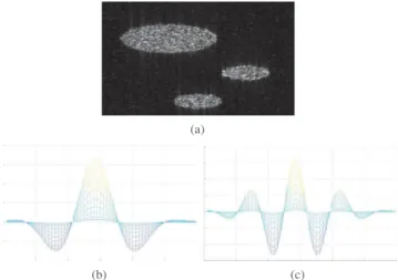
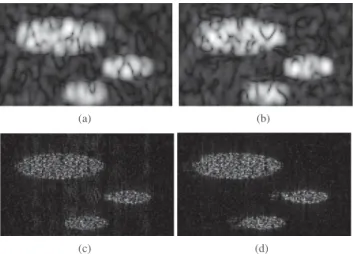
PSF and first harmonic PSF are shown in Figs. 3 (a, b, c) respec-tively. Figs. 4 (a, b) show the simulated observed B-mode image (log-compressed envelope image of the corresponding beamformed RF image commonly used for visualization purpose in US imaging) obtained from the TRF convolved with the two PSFs in baseband and arround the first harmonic respectively. The estimated TRF us-ing the classical US image restoration approach followus-ing (15) is shown in Fig. 4 (c) (forα = 0.01). Fig. 4 (d) displays the estimated TRF using the proposed method. The quality of the deconvolution can be appreciated by comparing the estimated TRFs obtained with the two methods. The density of the estimated TRF inside the inclu-sions is higher with the proposed method. Visual results are com-plemented by quantitative performance measures, i.e., by the struc-tural similarity (SSIM) [23] and the NRMSE (see Table1). The proposed method provides estimates of the imaged medium’s reflec-tivity that are closer to the reference image while taking advantage of the blurred data corresponding to the linear and the non-linear branches of the considered model.

(a)

(b) (c)

Fig. 3.(a) TRF phantom, (b, c) US PSF in baseband frequency and around the first harmonic (with baseband frequency f0= 3.5 MHz).

(a) (b)

(c) (d)

Fig. 4. (a, b) Blurred image with baseband and first harmonic PSF, (c) Estimated TRF using the classical approach for β= 0.0012, µ = σ2_and α= 0.01, (d) Estimated TRF using the proposed method.

Index α SSIM(%) NRMSE(%)

Proposed method - 97.10 0.68 Classical method [19] 0 97.16 0.69 0.01 97.05 0.69 0.05 93.22 0.87 0.1 83.14 1.38 0.5 32.55 7.01

Table 1. Performance measures for different values of the degree of non-linearityα

.

5. CONCLUSION

In presence of non-linearities affecting a medium of interest, stan-dard linear image processing techniques can have serious limitations leading to image anomalies. The origin of these anomalies is due to the fact that linear models cannot explain the non-linear interactions between the imaged medium and the observed image. This paper showed the interest of considering non-linear models and dedicated image processing strategies to estimate the tissue reflectivity from an ultrasound image. Our results are encouraging and open up new prospects. Future works will be devoted to apply the proposed ap-proach to in vivo data taking into consideration that the reflectivity depends on the type of the interaction between the tissues and the beamformed waves. It would be also interesting to consider blind deconvolution methods allowing a spatially variant PSF to be esti-mated.

6. REFERENCES

[1] T. L. Szabo, Diagnostic ultrasound imaging: inside out. Academic Press, 2004.

[2] N. Wagner, Y. C. Eldar, and Z. Friedman, “Compressed beamforming in ultrasound imaging,” IEEE Trans. Signal Process., vol. 60, no. 9, pp. 4643–4657, 2012.

[3] J. Du, D. Liu, and E. S. Ebbini, “Nonlinear imaging of microbubble contrast agent using the volterra filter: In vivo results,” IEEE trans-actions on ultrasonics, ferroelectrics, and frequency control, vol. 63, no. 12, pp. 2069–2081, 2016.

[4] O. V. Michailovich and D. Adam, “A novel approach to the 2-d blind deconvolution problem in medical ultrasound,” IEEE Trans. Med. Imag., vol. 24, no. 1, pp. 86–104, 2005.

[5] Z. Chen, A. Basarab, and D. Kouamé, “Reconstruction of enhanced ultrasound images from compressed measurements using simultaneous direction method of multipliers,” IEEE Trans. Ultrason., Ferroelect., Freq. Control, vol. 63, no. 10, pp. 1525–1534, Oct 2016.

[6] T. Taxt, “Restoration of medical ultrasound images using two-dimensional homomorphic deconvolution,” IEEE Trans. Ultrason., Ferroelect., Freq. Control, vol. 42, no. 4, pp. 543–554, 1995. [7] N. Zhao, Q. Wei, A. Basarab, N. Dobigeon, D. Kouamé, and J. Y.

Tourneret, “Fast single image super-resolution using a new analytical solution for ℓ2- ℓ2problems,” IEEE Trans. Image Process., vol. 25, no. 8, pp. 3683–3697, Aug 2016.

[8] A. Farina, “Simultaneous measurement of impulse response and distor-tion with a swept-sine technique,” in Audio Engineering Society Con-vention 108. Audio Engineering Society, 2000.

[9] A. Novak, L. Simon, F. Kadlec, and P. Lotton, “Nonlinear system iden-tification using exponential swept-sine signal,” IEEE Trans. Instrum. Meas., vol. 59, no. 8, pp. 2220–2229, 2010.

[10] M. Rébillat, R. Hennequin, E. Corteel, and B. F. Katz, “Identification of cascade of hammerstein models for the description of nonlinearities in vibrating devices,” Journal of sound and vibration, vol. 330, no. 5, pp. 1018–1038, 2011.

[11] F. Varray, A. Ramalli, C. Cachard, P. Tortoli, and O. Basset, “Fun-damental and second-harmonic ultrasound field computation of inho-mogeneous nonlinear medium with a generalized angular spectrum method,” IEEE Transactions on Ultrasonics, Ferroelectrics, and Fre-quency Control, vol. 58, no. 7, pp. 1366–1376, July 2011.

[12] M. Schetzen, “The Volterra and Wiener Theories of Nonlinear Sys-tems,” John Wiley, New-York, 1980.

[13] O. Nelles, Nonlinear System Identification: From Classical Approaches to Neural Networks and Fuzzy Models. Springer Science & Business Media, New-York, 2001.

[14] R. Haber and L. Keviczky, Nonlinear System Identification-Input-Output Modeling Approach. Kluwer Academic Publishers, 1999. [15] P. Crama and J. Schoukens, “Initial estimates of Wiener and

Hammer-stein systems using multisine excitation,” IEEE Trans. Instrum. Meas., vol. 50, no. 6, pp. 1791–1795, 2001.

[16] J. S. Bendat, Nonlinear Systems Techniques and Applications. John Wiley, New-York, 1998.

[17] A. Farina, A. Bellini, and E. Armelloni, “Non-linear convolution: A new approach for the auralization of distorting systems,” Amsterdam, The Netherlands, May 2001.

[18] R. Morin, S. Bidon, A. Basarab, and D. Kouamé, “Semi-blind decon-volution for resolution enhancement in ultrasound imaging,” in IEEE Proc. Int. Conf. Image Process. (ICIP), Melbourne, Australia, Feb. 2013.

[19] Z. Chen, A. Basarab, and D. Kouamé, “Compressive deconvolution in medical ultrasound imaging,” IEEE Trans. Med. Imag., vol. 35, no. 3, pp. 728–737, 2016.

[20] T. Taxt and R. Jirik, “Superresolution of ultrasound images using the first and second harmonic signal,” IEEE Transactions on Ultrasonics, Ferroelectrics, and Frequency Control, vol. 51, no. 2, pp. 163–175, Feb 2004.

[21] D. Gabay and B. Mercier, “A dual algorithm for the solution of nonlin-ear variational problems via finite element approximation,” Computers & Mathematics with Applications, vol. 2, no. 1, pp. 17–40, 1976. [22] S. Boyd, N. Parikh, E. Chu, B. Peleato, and J. Eckstein, “Distributed

op-timization and statistical learning via the alternating direction method of multipliers,” Foundations and Trends in Machine Learning, vol. 3, no. 1, pp. 1–122, 2011.

[23] Z. Wang, A. C. Bovik, H. R. Sheikh, and E. P. Simoncelli, “Image quality assessment: from error visibility to structural similarity,” IEEE Trans. Image Process., vol. 13, no. 4, pp. 600–612, 2004.