Experimental thermodynamic measurements of biofuel-related associating compounds and modeling using the PC-SAFT equation of state

HAL Id: pastel-00666125

https://pastel.archives-ouvertes.fr/pastel-00666125

Submitted on 3 Feb 2012

HAL is a multi-disciplinary open access

archive for the deposit and dissemination of

sci-entific research documents, whether they are

pub-lished or not. The documents may come from

teaching and research institutions in France or

abroad, or from public or private research centers.

L’archive ouverte pluridisciplinaire HAL, est

destinée au dépôt et à la diffusion de documents

scientifiques de niveau recherche, publiés ou non,

émanant des établissements d’enseignement et de

recherche français ou étrangers, des laboratoires

publics ou privés.

biofuel-related associating compounds and modeling

using the PC-SAFT equation of state

Chien-Bin Soo

To cite this version:

Chien-Bin Soo. Experimental thermodynamic measurements of biofuel-related associating compounds

and modeling using the PC-SAFT equation of state. Chemical and Process Engineering. École

Nationale Supérieure des Mines de Paris, 2011. English. �NNT : 2011ENMP0053�. �pastel-00666125�

T

H

È

S

E

INSTITUT DES SCIENCES ET TECHNOLOGIES

Ecole doctorale n

O

_{432 : Sciences des Métiers de l’Ingénieur}

Doctorat ParisTech

T H È S E

pour obtenir le grade de docteur délivré par

l’École Nationale Supérieure des Mines de Paris

Spécialité« Génie des Procédés »

présentée et soutenue publiquement par

Chien-Bin SOO

le 15 juin 2011

Mesures Expérimentales “Thermodynamiques” de Composés Associatifs dans

les Mélanges de Biocarburants et Modélisation avec l’Équation d’État PC-SAFT

Experimental Thermodynamic Measurements of Biofuel-related Associating

Compounds and Modeling using the PC-SAFT Equation of State

Directeur de thèse :Dominique RICHON

Co-directeur de thèse :Deresh RAMJUGERNATH

Jury

M. George JACKSON,Professor, Department of Chemical Engineering, Imperial College London Président

M. Theodoor W. DE LOOS,Associate Professor, Process & Energy Laboratory, TU Delft Rapporteur

M. Joachim GROß,Professor, ITT, University of Stuttgart Rapporteur

M. Jean-Charles DE HEMPTINNE,Professeur IFP School, IFP Energies nouvelles Examinateur

M. Kai FISCHER,Senior Research Thermodynamicist, Royal Dutch Shell Company Examinateur

M. Deresh RAMJUGERNATH,Professor, School of Chemical Engineering, UKZN Examinateur

M. Christophe COQUELET,Maître Assistant, CEP Fontainebleau/TEP, MINES ParisTech Examinateur

M. Dominique RICHON,Directeur de recherche, CEP Fontainebleau/TEP, MINES ParisTech Examinateur

MINES ParisTech

Centre Énergétique et Procédés - Laboratoire CEP/TEP

T

H

È

S

E

INSTITUT DES SCIENCES ET TECHNOLOGIES

Ecole doctorale n

O

_{432 : Sciences des Métiers de l’Ingénieur}

Doctorat ParisTech

T H È S E

pour obtenir le grade de docteur délivré par

l’École Nationale Supérieure des Mines de Paris

Spécialité« Génie des Procédés »

présentée et soutenue publiquement par

Chien-Bin SOO

le 15 juin 2011

Mesures Expérimentales “Thermodynamiques” de Composés Associatifs dans

les Mélanges de Biocarburants et Modélisation avec l’Équation d’État PC-SAFT

Experimental Thermodynamic Measurements of Biofuel-related Associating

Compounds and Modeling using the PC-SAFT Equation of State

Directeur de thèse :Dominique RICHON

Co-directeur de thèse :Deresh RAMJUGERNATH

Jury

M. George JACKSON,Professor, Department of Chemical Engineering, Imperial College London Président

M. Theodoor W. DE LOOS,Associate Professor, Process & Energy Laboratory, TU Delft Rapporteur

M. Joachim GROß,Professor, ITT, University of Stuttgart Rapporteur

M. Jean-Charles DE HEMPTINNE,Professeur IFP School, IFP Energies nouvelles Examinateur

M. Kai FISCHER,Senior Research Thermodynamicist, Royal Dutch Shell Company Examinateur

M. Deresh RAMJUGERNATH,Professor, School of Chemical Engineering, UKZN Examinateur

M. Christophe COQUELET,Maître Assistant, CEP Fontainebleau/TEP, MINES ParisTech Examinateur

M. Dominique RICHON,Directeur de recherche, CEP Fontainebleau/TEP, MINES ParisTech Examinateur

MINES ParisTech

Centre Énergétique et Procédés - Laboratoire CEP/TEP

 

 

 

 

 

 

 

 

 

 

 

獻給 我的母親

 

Acknowledgements

This thesis is a gift from my families, friends and colleagues, who gave me the love and support to see this

work through to the very end.

I would first like to thank my thesis director, Prof. Dominique Richon, for accepting me into the

prestigious establishment that is TEP, and my co-director, Prof. Deresh Ramjugernath, for promoting my

studies in Europe. I would like to mention the irreplaceable role of my maˆıtre assistant, Dr. Christophe

Coquelet, who dedicated his time to supervising my work and my interests. It has been a pleasure to work

with the lab staff and personnel of TEP, and I thank them for the friendship, the ambiance, and the energy

that they have brought to my daily life at Fontainebleau.

During my studies, I had the privilege of working abroad at different academic establishments. I

would like to thank Prof. Joachim Gross of the University of Stuttgart, without whom the modeling work

of this study would probably remain incomplete. I am indebted to his generosity for prolonging my

sabbatical at the ITT institute. Dr. Patrice Paricaud of ENSTA, who unselfishly shared his modeling

experiences, and to whom I had great pleasure in collaborating with. Dr. Jean-Yves Coxam and Dr. Karine

Ballerat-Busserolles of the University of Blaise-Pascal, for facilitating my calorimetry training at such

short notice. The staff and students at my alma mater, the University of KwaZulu-Natal, whose assistance

allowed me to maximize my experimental time in South Africa. A special mention must go to the Chang

family, who accommodated my visit there and treated me like their own. Finally, I would like to thank Iris

and David, who helped me with the French translations of the thesis. Without them, most of the French

parts in here would have been unreadable.

I would also like to acknowledge the financial supports of CARNOT MINES and SESAME for making

this research initiative possible. I am grateful to the members of the examining jury for their presence and

kind advice in the thesis defense.

To my very special group of friends:

Xavier

, for helping me during the difficult times when I arrived in France, and being my first friend

here. You reminded me that there is a life outside the thesis, and encouraged me to live it to the fullest.

Despite what people may tell you, you’re still the best Ph.D. I have met from our lab.

Paolo

, for showing me how to think laterally and maturely. It seems there is something to be learnt

from you everyday, not only how to be a better scientist, but to be a better person.

need (especially when my hard drive crashed, you still have my thanks!).

Ali

, for being a compassionate friend, giving to others without asking for anything in return. I’m sure

you’re going to succeed in becoming the professor that you wish to be.

V

, for being an amazing colleague and friend; for being understanding at all times. I couldn’t have

asked for better company, both within and outside work.

Xiaohua

, for all the excellent scientific advice you imparted towards the end of my thesis. You are

indeed the true PC-SAFT expert!

Diani

, for your prayers and your support. We may be distances apart, but your words of

encourage-ment reached me clear as ever. Thank you.

Vale

, for being a special friend and someone I could confide in. Knowing that you’re always there

to talk to, even into the early hours of the morning, made those long nights so much more bearable.

Shalen

, for keeping me sane on the weekends during second year. Thoroughly enjoyed our sessions

of toasted sandwiches, plastic 5 L kegs, Chinese buffets, and ridding the world of zombies. Good times.

Steve

, for the amazing friendship; for making it fifteen years, and counting.

Finally, I dedicate this thesis to my mother, who endured with me all the hardships over the past four

years. Mama, you loved me unconditionally, no matter what the result was. This is the result, and it is for

you.

Fontainebleau, June 2011

Contents

List of Figures

List of Tables

Introduction

1

1

Biofuel as a Global Initiative

5

1.1 A brief history of oil

. . . .

9

1.2 The debate for alternative energy

. . . .

11

1.3 Renewable energy processes

. . . .

15

1.4 Major climate change initiatives

. . . .

18

1.5 Biofuel review and production

. . . .

21

1.5.1

Definition and characterization of biofuels

. . . .

21

1.5.2

The cases for and against biofuels

. . . .

23

1.5.3

Bioethanol

. . . .

26

1.5.4

Ethyl tert-butyl ether (ETBE)

. . . .

29

1.5.5

Biodiesel and vegetable oil esters

. . . .

30

1.5.6

Pyrolysis Oil

. . . .

32

1.6 Thermodynamics in biofuel research: an example

. . . .

34

1.7 Industrial context and thesis objectives

. . . .

37

2

Fundamentals of the Perturbed-Chain Statistical Associating Fluid Theory (PC-SAFT)

39

2.1 Intermolecular forces in nature

. . . .

43

2.1.1

Physical forces

. . . .

44

2.1.2

Hydrogen Bonding

. . . .

46

2.1.3

Intermolecular potential functions

. . . .

46

2.2 Perturbation theory in equation of states

. . . .

49

2.2.1

The radial distribution function

. . . .

49

2.2.2

First and second-order perturbation expansions

. . . .

50

2.3 Residual Helmholtz contributions of the PC-SAFT

. . . .

51

2.3.1

Wertheim’s TPT1 theory and the association term

. . . .

51

2.4 Systematic parameterization of the PC-SAFT

. . . .

62

2.5 Concluding remarks

. . . .

65

3

Vapour-liquid equilibrium measurements of binary systems

67

3.1 Low pressure vapour-liquid equilibria by a “dynamic-analytic” method

. . . .

71

3.1.1

Overview

. . . .

71

3.1.2

Description of the dynamic-analytic apparatus

. . . .

71

3.1.3

Experimental procedures

. . . .

73

3.1.4

Estimation of uncertainty for low pressure measurements

. . . .

79

3.1.5

Results of low pressure vapour-liquid equilibrium measurements

. . . .

82

3.2 High pressure vapour-liquid equilibria by a “static-analytic” method

. . . .

86

3.2.1

Overview

. . . .

86

3.2.2

Description of the static-analytic apparatus

. . . .

88

3.2.3

Experimental procedures

. . . .

90

3.2.4

Estimation of uncertainty for high pressure measurements

. . . .

92

3.2.5

Results of high pressure vapour-liquid equilibrium measurements

. . . .

94

3.3 Concluding remarks

. . . .

95

4

Experimental determination of critical points using a “dynamic-synthetic” apparatus

99

4.1 Description of “dynamic-synthetic” apparatus

. . . 103

4.2 Experimental procedures

. . . 105

4.3 Results and discussions

. . . 107

4.4 Recommendations for the apparatus

. . . 117

4.5 Concluding remarks

. . . 120

5

Thermodynamic modeling of biofuel systems using the PC-SAFT equation of state

121

5.1 Modeling aspects and approach

. . . 125

5.2 Application of the PC-SAFT in modeling fluid phase equilibria of polar mixtures

. . . . 126

5.2.1

Alcohols

. . . 126

5.2.2

Carboxylic acids

. . . 132

5.2.3

Polar Compounds

. . . 142

5.2.4

Aqueous mixtures and other compounds

. . . 152

5.3 Calculation of Excess Enthalpy

. . . 160

5.4 Thermodynamic Consistency Testing

. . . 164

5.4.1

Methods and Test Criteria

. . . 165

5.4.2

Results of tests

. . . 166

6

Modeling aspects of the PC-SAFT in the critical region

173

6.1 Recursive renormalization procedure for mixtures

. . . 177

6.1.1

Phase-space cell approximation

. . . 178

6.1.2

Isomorphic approximation

. . . 179

6.1.3

Parameterization of the PC-SAFT-RG

. . . 180

6.2 Results and Discussion

. . . 183

6.2.1

Pure components

. . . 183

6.2.2

Binary mixtures

. . . 183

6.3 Concluding remarks

. . . 192

Conclusions and Prospective Work

195

Bibliography

205

Appendices

224

A Determination of excess enthalpy by calorimetry

225

A.1 The Setaram Calvet Calorimeters

. . . 225

A.2 Description of the apparatuses

. . . 226

A.3 Calibration of equipment

. . . 228

A.4 Experimental procedures

. . . 232

A.5 Results and discussion

. . . 234

B Analytical derivatives of the PCIP-SAFT equation of state

237

C Table of results for vapour-liquid equilibrium measurements

257

D Worked example illustrating the estimation of uncertainties

265

E Table of results for critical point measurements

273

F Communications

277

1.1 Distribution of the world’s proven oil reserves at the end of 2009

. . . .

10

1.2 Year to year changes of oil prices from 1981 to 2007

. . . .

11

1.3 Graphs showing the trends of atmospheric CO

2

, global population, energy consumption

and global temperature for the past decades

. . . .

13

1.4 Global reserves-to-production ratio at the end 2009

. . . .

14

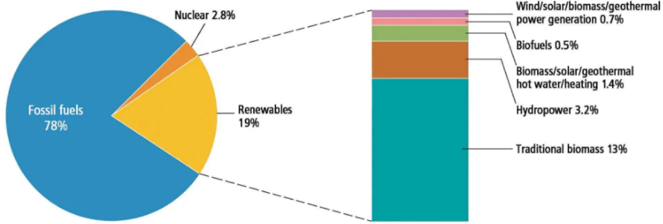
1.5 Share of renewable energy in the global final energy consumption for the year 2008

. . .

15

1.6 Market share of biofuels of some member states of the European Directive 2003/30/EC

.

21

1.7 Top global producers of bioethanol and biodiesel at the end of 2009

. . . .

22

1.8 Carbon cycle with biomass as the energy source

. . . .

24

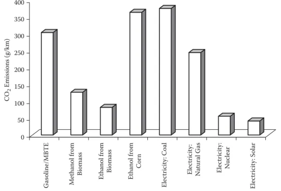
1.9 Comparisons of the CO

2

emissions between corn ethanol and other forms of energy

. . .

25

1.10 Inflated adjusted price per bushel of corn in the US over the past thirty years

. . . .

26

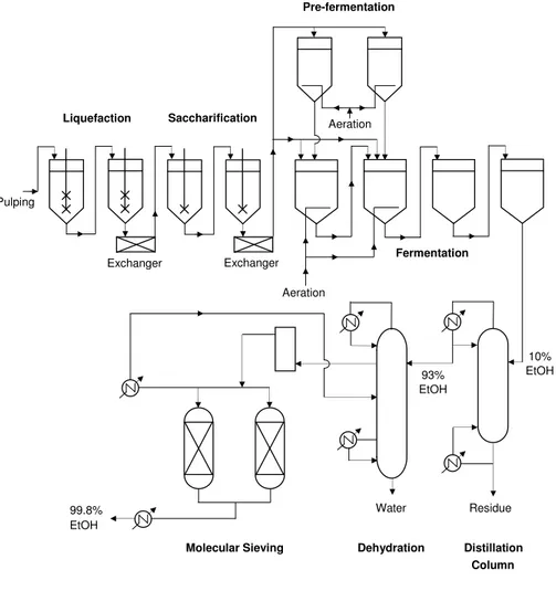
1.11 Process flow diagram of ethanol production via the dry milling process

. . . .

27

1.12 Vapour pressures of volumetric additions of ethanol in a generic gasoline

. . . .

28

1.13 Synthesis reaction of ETBE from isobutene and ethanol

. . . .

29

1.14 Process flow diagram of ETBE production

. . . .

30

1.15 Transesterification reaction of alkyl esters from triglyceride and alcohol. R

i

can be any

alkyl group.

. . . .

30

1.16 Process flow diagram of methyl ester production proposed by IFP

. . . .

32

1.17 Fractionation scheme for analysis of pyrolysis oil, using water and vacuum filtration

. . .

33

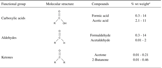
1.18 Examples of multi-functional, oxygenated compounds found in pyrolysis oil

. . . .

33

1.19 A simplified strategy cycle for the design of chemical processes

. . . .

34

1.20 Vapour-liquid equilibria modeling of binary pairs of the ETBE + ethanol + benzene system

36

1.21 Predictions of vapour-liquid equilibria for the toluene + acetic acid system using the PSRK

and modified UNIFAC model

. . . .

38

2.1 Intermolecular attractions between toluene and acetone molecules

. . . .

44

2.2 Radial distribution function of oxygen-oxygen atoms in liquid water

. . . .

49

2.3 Model approximations of Wertheim’s association theory

. . . .

53

2.4 Geometric representations of the 2CLJ and TS model

. . . .

60

2.5 Geometric representations of a dipolar chain molecule under the JC and GV approach

. .

63

3.1 Illustration of the “dynamic-analytic” apparatus used for measurements of low pressure

vapour-liquid equilibria

. . . .

74

3.2 Calibration of the Pt-100 temperature probe for the “dynamic-analytic” apparatus

. . . .

75

3.3 Calibration of the pressure transducer for the dynamic-analytic apparatus

. . . .

75

3.4 TCD Calibration for the ethanol + cyclohexane system using the method of Raal and

M¨uhlbauer

. . . .

77

3.5 GC chromatograms showing an impurity peak conflicting undesirably with main peaks

.

78

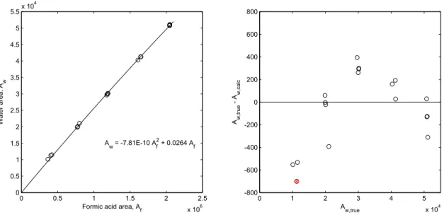
3.6 Water peak area as a function of the peak area of formic acid A

f

. . . .

78

3.7 Pure component vapour pressures for compounds studied in low pressure vapour-liquid

equilibria

. . . .

83

3.8 Experimental VLE data for the ethanol + cyclohexane binary system

. . . .

84

3.9 Experimental VLE data for the n-hexane + 1-propanol binary system

. . . .

85

3.10 Experimental VLE data for the ethanol + m-xylene binary system at 95 kPa

. . . .

85

3.11 Experimental VLE data for the ethanol + m-xylene binary system at 323 - 343 K

. . . .

86

3.12 Experimental VLE data for the ethanol + ethylbenzene binary system

. . . .

86

3.13 Experimental VLE data for the benzene + acetic acid binary system

. . . .

87

3.14 Experimental VLE data for the toluene + acetic acid binary system

. . . .

87

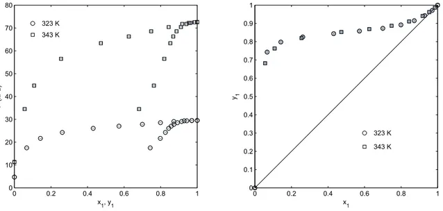
3.15 Experimental VLE data for the acetone + formic acid binary system

. . . .

88

3.16 Flow diagram of “static-analytic” apparatus used for measurements of high pressure

vapour-liquid equilibria

. . . .

89

3.17 Calibration of the pressure transducer for the static-analytic apparatus

. . . .

91

3.18 TCD calibration for ethanol, performed using direct syringe injections

. . . .

91

3.19 Experimental VLE data for the propane + ethanol binary system

. . . .

96

3.20 Experimental VLE data for the n-butane + ethanol binary system

. . . .

97

4.1 Flow diagram of “dynamic-synthetic” apparatus used for critical point measurements

. . 104

4.2 Calibration of the pressure transducer for the critical point apparatus

. . . 106

4.3 Calibration of the Pt-100 temperature probe for the critical point apparatus

. . . 106

4.4 Transition of a fluid mixture to the critical state during measurement

. . . 107

4.5 Temperature and pressure profiles during the measurement of critical points

. . . 108

4.6 Experimental critical pressures and temperatures for the propane + n-butane system

. . . 112

4.7 Experimental critical pressure and temperature profiles for the n-butane + ethanol system

112

4.8 Experimental critical pressures and temperatures for the n-pentane + ethanol system

. . . 113

4.9 Experimental critical pressures and temperatures for the ethanol + n-hexane system

. . . 113

4.10 Experimental critical pressures and temperatures for the ethanol + n-heptane system

. . . 113

4.11 Experimental critical pressures and temperatures for the ethanol + n-octane system

. . . 114

4.12 Experimental critical pressures and temperatures for the ethanol + 1-propanol system

. . 114

4.13 Experimental critical pressures and temperatures for the propane + R134a system

. . . . 114

4.14 Experimental critical pressures and temperatures for the n-pentane + n-hexane system

. . 116

4.15 Experimental critical pressures and temperatures for the n-pentane + ethanol + n-hexane

system

. . . 117

5.2 VLE modeling results for the propane + ethanol system from 325-403 K

. . . 128

5.3 VLE modeling results for the n-butane + ethanol system from 325-453 K

. . . 128

5.4 VLE modeling results for the n-butane + methanol system from 323-443 K

. . . 129

5.5 VLE modeling results for the ethanol + cyclohexane system at 100 kPa and 323 K

. . . . 130

5.6 VLE modeling results for the n-hexane + 1-propanol system at various isotherms and isobar

131

5.7 VLE modeling results for the ethanol + m-xylene system at various isotherms and isobar

131

5.8 VLE modeling results for the ethanol + ethylbenzene system at 323 and 343 K

. . . 132

5.9 VLE modeling results for the cyclohexane + cyclohexanol system from 424-484 K

. . . 133

5.10 VLE modeling results for the cyclohexane + cyclohexanol system from 298-328 K

. . . 133

5.11 Saturated vapour pressures and liquid densities for chain acids

. . . 137

5.12 VLE modeling results for the benzene + acetic acid system at 323 K

. . . 137

5.13 VLE modeling results for the benzene + acetic acid system from 313-343 K

. . . 138

5.14 VLE modeling results for the cyclohexane + n-hexanoic acid system from 413-484 K

. . 138

5.15 VLE modeling results for the formic acid + acetic acid system at 101 kPa and 343 K

. . 139

5.16 VLE modeling results for the acetic acid + propionic acid system at 101 kPa and 343 K

. 139

5.17 Effect of the k

12

parameter on the representation of the acetic acid + n-octane system

. . 140

5.18 VLE modeling results for the acetic acid + n-octane system at 323 and 343 K

. . . 141

5.19 VLE modeling results for the toluene + acetic acid and cyclohexane + acetic acid systems

141

5.20 VLE modeling results for the 1-butanol + acetic acid and 1-butanol + butanoic acid systems

142

5.21 Cross-association (solvation) between an ether and an alcohol molecule

. . . 143

5.22 VLE modeling results for the acetone + cyclohexane system at 298-323 K

. . . 144

5.23 VLE modeling results for the n-pentane + acetone system at 373-423 K

. . . 144

5.24 VLE modeling results for the cyclohexane + cyclohexanone system at various temperatures

145

5.25 VLE modeling results for the acetone + 2-butanone system at various pressures

. . . 145

5.26 VLE modeling results for the acetic acid + acetone and 2-butanone + propanoic acid systems

146

5.27 VLE modeling results for the isobutene + ETBE and ETBE + benzene systems

. . . 146

5.28 VLE modeling results for the 1-hexene + ETBE + benzene ternary system

. . . 147

5.29 VLE modeling results for the ETBE + ethanol system from 298-363 K

. . . 148

5.30 Calculation of saturated vapour pressures and liquid densities for FAME

. . . 149

5.31 Calculation of latent heats of vaporization and surface tensions for FAME

. . . 151

5.32 VLE modeling results for the methyl myristate + methyl palmitate and methyl laurate +

methyl myristate systems

. . . 151

5.33 VLE modeling results for the methanol + methyl laurate and methanol + methyl myristate

systems from 493-543 K

. . . 153

5.34 VLE modeling results for the toluene + furfural and n-hexane + furfural systems

. . . . 154

5.35 VLE modeling results for the acetaldehyde + acetic acid and acetaldehyde + 2-propanol

systems

. . . 154

5.36 PC-SAFT modeling results for the water + 1-butanol and water + acetic acid systems

. . 155

5.38 PC-SAFT modeling results for the water + butyraldehyde and furfural + 2-butanone +

water systems

. . . 157

5.39 PC-SAFT modeling results for the toluene + phenol and n-octane + phenol systems

. . . 158

5.40 VLE modeling results for the anisole + phenol and n-hexane + anisole systems

. . . 160

5.41 LLE modeling results for the acetone + guaiacol and m-cresol + water systems

. . . 160

5.42 VLE modeling results for the alcohols + glycerol and water + glycerol systems

. . . 161

5.43 LLE modeling results for the methyl oleate + methanol + glycerol ternary system

. . . . 161

5.44 VLE and h

E

_{modeling for the n-hexane + cyclohexane system}

_{. . . 162}

5.45 h

E

_{modeling for the ethanol + benzene system}

_{. . . 163}

5.46 VLE and h

E

_{modeling for the methanol + 1-octanol and ETBE + n-heptane systems}

_{. . . 164}

5.47 h

E

_{modeling for acetone + n-alkane and ETBE + ethanol systems}

_{. . . 165}

5.48 Examples of the thermodynamic consistency tests used in this work

. . . 169

6.1 Recursive renormalization of long-range density fluctuations

. . . 178

6.2 Vapour pressures and coexisting densities of ethanol, 1-propanol and R134a

. . . 184

6.3 Evolution for the triple sum criteria using the PC-SAFT and PC-SAFT-RG

. . . 185

6.4 PC-SAFT and PC-SAFT-RG-PS modeling results for the n-butane + methanol system at

423 and 443 K

. . . 186

6.5 Modeling of mixture VLE and critical point data using PC-SAFT and PC-SAFT-RG for

the propane + n-butane system

. . . 187

6.6 Response of mixture critical points to changes in the k

12

binary parameter

. . . 188

6.7 Critical line modeling of the propane + n-butane and n-pentane + n-hexane systems

. . . 188

6.8 Critical line modeling of the n-butane + ethanol system

. . . 189

6.9 Critical line modeling of the n-pentane + ethanol and ethanol + n-hexane systems

. . . . 190

6.10 Critical line modeling of the ethanol + n-heptane and ethanol + n-octane systems

. . . . 191

6.11 Critical line modeling of the ethanol + 1-propanol and propane + R134a systems

. . . . 191

I

Schematic drawing of new LLE cell at CEP/TEP laboratory

. . . 196

A.1 Components of the stainless steel membrane mixing cell

. . . 227

A.2 Schematic diagram of the BT2.15 calorimeter and its external circuit setup

. . . 229

A.3 Illustration of chemical calibration for liquid-liquid h

E

_measurements

_{. . . 231}

A.4 Snapshot of an experimental acquisition in static mode measurement of excess enthapy

. 232

A.5 Illustration of an q-t profile for an arbitrary system measured under the “dynamic” mode

233

A.6 Excess molar enthalpies for the cyclohexane + n-hexane and ethanol + n-hexane systems

234

A.7 Excess molar enthalpies for the water + triethylene glycol system at 298 K and 101 kPa

. 235

1.1 Significant dates in the history of oil price fluctuations

. . . .

12

1.2 Past predictions of the occurrence of the global oil peak

. . . .

14

1.3 Comparison of forms of renewable energies

. . . .

17

1.4 Optimal scenario of alternative fuels introduction until 2020 according to the EU

. . . .

20

1.5 Comparisons between ETBE, ethanol, and standard gasoline

. . . .

29

1.6 Comparison between catalytic and non-catalytic transesterification

. . . .

31

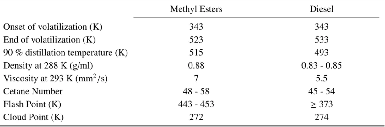
1.7 Comparison of the physical and performance properties between methyl esters & diesel

.

32

1.8 Overview of oxygenated functional groups in pyrolysis oils

. . . .

34

1.9 Binary interaction parameters for three different forms of PR EoS of increasing complexity,

for the systems ETBE + ethanol + benzene

. . . .

36

2.1 Reduced thermodynamic property relations for Helmholtz energy equation of states

. . .

52

3.1 Binary systems measured by the “dynamic-analytic” apparatus for low pressure

vapour-liquid equilibria

. . . .

72

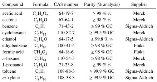
3.2 Purity and supplier of the compounds used in the measurement of low pressure

vapour-liquid equilibria

. . . .

72

3.3 GC column temperatures for each of the measured, low pressure binary systems

. . . . .

73

3.4 Averaged temperature, pressure, and mole fraction uncertainties for low pressure

vapour-liquid equilibria

. . . .

83

3.5 Binary systems measured by the “static-analytic” apparatus for high pressure vapour-liquid

equilibria

. . . .

88

3.6 Purity and supplier of the compounds used in the measurement of high pressure

vapour-liquid equilibria

. . . .

88

3.7 Averaged temperature, pressure, and mole fraction uncertainties for high pressure

vapour-liquid equilibria

. . . .

95

4.1 Purity and supplier of the compounds used in the measurement of critical points

. . . 104

4.2 Experimental critical temperatures of pure compounds

. . . 109

4.3 Experimental critical pressures for pure compounds

. . . 109

4.4 Comparison between experimental and predicted critical properties of R1216, C

₃

F

₆

O and

R365mfc

. . . 110

4.5 Redlich-Kister constants for binary mixture critical points measured in this work

. . . . 115

4.6 α and β constants for the n-pentane + ethanol + n-hexane ternary mixture

. . . 118

5.1 Abbreviations for the different variants of PC-SAFT EoS used in Chapter 5

. . . 125

5.2 Pure component parameters for carboxylic acids used in this work.

. . . 136

5.3 Pure component PC-SAFT parameters for ethyl-tert-butyl-ether (ETBE)

. . . 147

5.4 Pure component PC-SAFT parameters for fatty acid methyl esters

. . . 150

5.5 Pure component PC-SAFT parameters for phenolics and miscellaneous compounds

. . . 159

5.6 Results of the thermodynamic consistency tests for the binary systems measured in this work

168

5.7 Summary of the modeling approaches adopted in this work for modeling mixtures of

oxygenated compounds

. . . 171

6.1 PC-SAFT-RG parameters used for this work

. . . 182

6.2 Critical properties of compounds with new parameters determined in this work for the

PC-SAFT-RG

. . . 183

6.3 Comparison between PC-SAFT and PC-SAFT-RG in modeling mixture critical points

. . 192

A.1 Excess molar enthalpies for the cyclohexane + n-hexane and ethanol + n-hexane systems

235

B.1 Quick referencing of the derivatives presented in Appendix B

. . . 238

C.1 Vapour-liquid equilibrium measurements for the ethanol + cyclohexane system

. . . 257

C.2 Vapour-liquid equilibrium measurements for the n-hexane + 1-propanol system

. . . 258

C.3 Vapour-liquid equilibrium measurements for the ethanol + m-xylene system

. . . 258

C.4 Vapour-liquid equilibrium measurements for the ethanol + ethylbenzene system

. . . 259

C.5 Vapour-liquid equilibrium measurements for the benzene + acetic acid system

. . . 259

C.6 Vapour-liquid equilibrium measurements for the toluene + acetic acid system

. . . 260

C.7 Vapour-liquid equilibrium measurements for the acetone + formic acid system

. . . 261

C.8 Vapour-liquid equilibrium measurements for the propane + ethanol system

. . . 261

C.9 Vapour-liquid equilibrium measurements for the n-butane + ethanol system

. . . 262

D.1 Experimental records of the first equilibrium condition for the propane + ethanol system,

at 343 K

. . . 268

D.2 Calculation of the uncertainties on molar composition, due to imprecisions in the

calibra-tion procedure, for both the liquid and vapour samples.

. . . 270

E.1 Experimental critical temperatures and pressures for binary mixtures

. . . 273

E.2 Experimental critical temperatures and pressures for the n-pentane + ethanol + n-hexane

mixture

. . . 276

Introduction

Accurate experimental data

and reliable thermodynamic models are basic requirements for cost-effective

and safe process design. In this thesis, both these aspects are addressed in the context of a novel energy

source - biological fuels. When considered as a transportation fuel or chemical intermediate, biofuels

are unique through its ensemble of oxygenated compounds, exhibiting the type of interactions and phase

equilibria not encountered as frequently in petroleum engineering applications. As a technology in

development, the integration of biofuels on a process level relies heavily on the two fundamentals which

form the central themes of this work: the acquisition of thermo-physical data; and a means to model

complex molecular interactions.

The aim of the thesis is to address this seemingly two-part conundrum in each of the experimental and

modeling sections. Biofuel is first introduced as an energy alternative, in which its positive and negative

impacts on the ecosystems are critically reviewed. By examining the chemistry of bioethanols, biodiesels

and biomass oils, the oxygenated compounds to be studied in this work is brought to the fore. The thesis

focuses mainly on the first generation biofuels. The following chapter highlights the behaviour of real

fluids that exhibit both physical and quasi-chemical interactions. The identification of pertinent forces in

oxygenated compounds provides the justification for adopting a SAFT-type approach in the later modeling

part of the work. The second chapter ends with a review of the Helmholtz free energy terms in the model

of choice, the PC-SAFT equation of state.

The crux of the work begins in the third, and first of two experimental chapters. In this chapter,

new vapour-liquid equilibrium data, at pressures ranging from 0.01 to 5 MPa, were measured for nine

systems including alkanes, alcohols, acids, and ketones. For pressures up to atmospheric conditions, the

measurements were effectuated using an ebulliometer-type apparatus based on the “dynamic-analytic”

method. At conditions above atmospheric, an apparatus based on the “static-analytic” method, with

two electromagnetic ROLSI

™

_{capillary samplers, was employed. The features of both apparatuses were}

examined as means of obtaining reliable experimental data, which have been shown to be valid.

In the fourth chapter, an efficient and reliable “dynamic-synthetic” method is proposed for the

measure-ment of critical properties of a variety of pure compounds, binary mixtures, and one ternary mixture. The

critical phenomenon is observed via the critical opalescence in a view cell, which withstands conditions

up to 543 K and 20 MPa. The apparatus incorporates a slight modification to commonly documented

procedures, with promising results. Excellent agreements were obtained between the measured pure

compounds’ properties and those listed in recent databases. Accurate critical data provides a reference

to which modeling work on SAFT-type equations, which lack constraints in the critical region, can be

developed.

PC-SAFT equation of state to polar and associating mixtures. Dealing mainly with fluid phase equilibria,

we examine the manner in which different non-idealities shown by various oxygenated compounds can be

approached by utilizing the available variants of PC-SAFT. The chapter proceeds to discuss the modeling

of excess enthalpies and thermodynamic consistency testing with the equation of state.

The final and sixth chapter deals with the modeling aspects in the critical region. To account for

long-range density fluctuations in the critical region, renormalization group corrections, according to

White, are applied to the PC-SAFT equation of state. The result is a model which scales correctly at

the critical point, and could be used to model the critical data obtained experimentally. Where critical

properties were originally over-estimated, the renormalization group corrections bring about significant

improvements in the description of the critical region.

Introduction

Des donn´ees exp´erimentales pr´ecises et des mod`eles thermodynamiques fiables sont des conditions de

base pour la conception de proc´ed´es rentables et fonctionnant en toute s´ecurit´e. Dans cette th`ese, ces

deux aspects sont abord´es dans le cadre d’une source d’´energie originale via les biocarburants. Si l’on

s’int´eresse aux carburants de transport ou aux interm´ediaires chimiques, les biocarburants sont uniques par

l’ensemble des compos´es oxyg´en´es qu’ils contiennent, pr´esentant des types d’interactions et d’´equilibres

de phase que l’on ne rencontre pas fr´equemment dans des applications li´ees `a l’ing´enierie p´etroli`ere.

Comme technologie `a l’´etude, l’int´egration des biocarburants au niveau proc´ed´e se base fortement sur les

deux principes fondamentaux qui forment les th`emes centraux de ce travail : l’acquisition de donn´ees

thermo-physiques; et des moyens de mod´eliser des interactions mol´eculaires complexes.

Le but de la th`ese est s’int´eresser `a cette apparente ´enigme en deux parties dans chacune des sections

exp´erimentales et mod´elisation. Les biocarburants sont tout d’abord pr´esent´es comme une ´energie

alternative, dans laquelle ses impacts positifs et n´egatifs sur les ´ecosyst`emes sont pass´es en revue de

mani`ere critique. Suite `a l’examen de la chimie des bio´ethanols, biodiesels et huiles de biomasse, les

compos´es oxyg´en´es `a ´etudier dans ce travail sont mis en lumi`ere. La th`ese se concentre principalement sur

les biocarburants de premi`ere g´en´eration. Le chapitre suivant pointe le comportement des fluides r´eels

qui pr´esentent des interactions physique et quasi-chimique. L’identification des forces pertinentes pour la

repr´esentation des compos´es oxyg´en´es fournit la justification pour adopter une approche de type SAFT

dans la partie de mod´elisation du travail. Le deuxi`eme chapitre se termine par l’examen des termes de

l’´energie libre de Helmholtz dans le mod`ele retenu, l’´equation d’´etat PC-SAFT.

L’essentiel du travail commence dans le troisi`eme, et le premier des deux chapitres exp´erimentaux.

Dans le chapitre 3, de nouvelles donn´ees d’´equilibres liquide-vapeur ont ´et´e mesur´ees pour des pressions

s’´etendant de 0.01 ´a 5 MPa sur neuf syst`emes comprenant des alcanes, des alcools, des acides, et des

c´etones. Aux pressions atmosph´eriques et subatmosph´eriques, les mesures ont ´et´e effectu´ees au moyen

d’un ´ebulliom`etre bas´e sur la m´ethode “dynamique-analytique”. Pour les pressions sup´erieures `a la

pression atmosph´erique, nous avons utilis´e un appareil bas´e sur la m´ethode “statique-analytique”, faisant

appel `a deux ´echantillonneurs ´electromagn´etiques `a capillaires ROLSI

™

_{. Les caract´eristiques des deux}

appareils ont ´et´e examin´ees en tant que moyens d’obtenir les donn´ees exp´erimentales fiables, ce qui a

permis de les d´eclarer aptes.

Dans le quatri`eme chapitre, on propose une m´ethode “dynamique-synth´etique” efficace et fiable pour

la mesure des propri´et´es critiques d’une s´erie de compos´es purs, de m´elanges binaires, et d’un m´elange

ternaire. On observe le ph´enom`ene critique par l’interm´ediaire de l’opalescence critique dans une cellule

transparente, conc¸ue pour r´esister jusqu`a 543 K et `a 20 MPa. L’appareil incorpore une l´eg`ere modification

aux proc´edures g´en´eralement d´ecrites, avec des r´esultats prometteurs. D’excellents accords ont ´et´e obtenus

entre les propri´et´es des compos´es purs ´etudi´es et celles ´enum´er´ees dans les bases de donn´ees r´ecentes.

Les donn´ees critiques pr´ecises fournissent une r´ef´erence sur laquelle un travail de mod´elisation par les

´equations de type SAFT, qui manquent de contraintes dans la r´egion critique, peut ˆetre d´evelopp´e.

Le cinqui`eme chapitre se concentre sur la mod´elisation des syst`emes de biocarburants, incluant les

valeurs exp´erimentales mesur´ees dans la premi`ere partie et autres. Le premier des deux chapitres de

mod´elisation est une ´etude syst´ematique de l’application de l’´equation d’´etat PC-SAFT aux m´elanges

polaires et associatifs. Traitant principalement les ´equilibres de phases fluides, nous examinons la fac¸on

dont diff´erentes non-id´ealit´es pr´esent´es par divers compos´es oxyg´en´es peuvent ˆetre approch´ees en utilisant

les variantes disponibles de PC-SAFT. Le chapitre se poursuit avec la discussion de la mod´elisation des

enthalpies d’exc`es et des tests de coh´erence via une ´equation d’´etat.

Le sixi`eme chapitre qui est le chapitre final traite les aspects de mod´elisation dans la r´egion critique.

Pour tenir compte des fluctuations de densit´e `a longue port´ee dans la r´egion critique, des corrections de

groupe de renormalisation, selon White, sont appliqu´ees `a l’´equation d’´etat PC-SAFT. Le r´esultat est un

mod`ele satisfaisant au point critique qui peut ˆetre employ´e pour mod´eliser les donn´ees critiques obtenues

exp´erimentalement. L`a o`u des propri´et´es critiques ont ´et´e `a l’origine surestim´ees, les corrections de groupe

de renormalisation conduisent `a des am´eliorations significatives de la description de la r´egion critique.

CHAPTER

1

Biofuel as a Global Initiative

The use of vegetable oils for engine fuels may seem insignificant today. But such oils may

become in course of time as important as petroleum and the coal tar products of the present

time.

- Rudolf Christian Karl Diesel (1858-1913)

Biocarburant, une initiative globale

Ce premier chapitre introduit le rˆole des biocarburants comme une ´energie renouvelable. Tout d’abord, un bref historique concernant les carburants d’origines fossiles est pr´esent´e - ressources d’´energie qui ont servi la communaut´e durant plusieurs d´ecennies. Bien que leur importance soit essentielle, leurs utilisations ont ´et´e r´ecemment mal g´er´ees conduisant `a des impacts sociaux tr`es n´egatifs. Quelques exemples notables sont : les ´emissions de gaz `a effet de serre, la propri´et´e non-renouvelable, un prix mon´etaire instable, et une forte implication politique.

Des d´ebats ont amen´e certains pays `a engager des initiatives afin de r´eduire leur d´ependance aux carburants d’origines fossiles. Une ´energie alternative envisageable doit ˆetre renouvelable, dans le sens qu’elle est naturellement recyclable, avec une empreinte carbone n´egligeable. Ce chapitre recense plusieurs types d’´energies renouvelables, incluant l’´energie issue de la biomasse, l’´energie solaire, celle du vent, la g´eothermie et l’´energie hydro´electrique. Le niveau d’int´egration des ´energies alternatives dans le march´e est d´efini par les l´egislations multinationales, tel que le Kyoto Protocol de 1997 et la directive europ´eenne. Le premier vise `a r´eduire grandement l’´emission mondiale de gaz `a effet de serre (CO2, CH4, N2O, SF6, HFC et PFC) pour 2012. Le dernier se focalise notamment sur les ´emissions provenant du secteur des transports afin de promouvoir l’utilisation de carburants issus de la biomasse -une source d’´energie qui est le th`eme centrale de ce travail.

Les biocarburants sont issus de mati`ere organique v´eg´etale et pr´esentent un int´erˆet particulier grˆace `a leur polyvalence. Ils sont quasiment neutres en carbone, puisque le dioxyde de carbone lib´er´e lors de sa combustion est r´eabsorb´e par les plantes pour leur croissance. Ils sont divis´es en plusieurs g´en´erations, selon la nature de la mati`ere premi`ere utilis´ee dans la production. Ce travail ´etudie principalement les biocarburants de premi`ere g´en´eration, qui extraient leur source d’´energie `a partir de sucres, de l’amidon et d’huiles v´eg´etales. Les biocarburants de premi`ere g´en´eration comprennent les carburants utilis´es pour le transport - le bio´ethanol, l’ETBE et le biodiesel. Les biocarburants de deuxi`eme g´en´eration sont d´eriv´es des parties non comestibles des plantes, comme la bio-huile et le biobutanol. Un type de biocarburants de troisi`eme g´en´eration, ´egalement connu comme carburants des algues, sera examin´e bri`evement ci-apr`es.

Il est important de noter que les biocarburants, comme les autres ´energies renouvelables, ne sont pas sans inconv´enients. Certains types de mati`eres premi`eres n’ont pas un potentiel ´egal de r´eduction de carbone et peuvent mˆeme contribuer `a d’autres ´emissions nocives, telles que le formald´ehyde. La promotion des biocarburants dans certains pays peut rivaliser avec les ressources alimentaires provoquant ainsi une augmentation des prix. Si la culture des plantes pour les biocarburants r´esulte `a la d´eforestation et `a des dommages `a l’´ecosyst`eme, les avantages des biocarburants sont r´eduits de mani`ere importante. Par cons´equent, une planification sociale et environnementale est n´ecessaire pour maximiser les effets positifs des biocarburants.

Une revue bibliographique sur la production des biocarburants est donn´ee dans le chapitre I, afin d’identifier les principaux types de proc´ed´es de s´eparation. Il est clair que les s´eparations thermiques et m´ecaniques sur un large assortiment de compos´es sont concern´ees. Il est n´ecessaire d’´etudier le comportement de phase des alcools (le bio´ethanol et biobutanol), des ´ethers (l’ETBE), des esters (biodiesel) et des acides carboxyliques (bio-huile), qui sont en m´elange avec des compos´es du p´etrole tels que des hydrocarbures, des aromatiques et des c´etones.

Pour la conception et la simulation efficace des proc´ed´es de production de biocarburants, l’importance des donn´ees exp´erimentales et des mod`eles thermodynamiques ne peut ˆetre n´eglig´ee. L’introduction d’un large assorti-ment de compos´es oxyg´en´es assorti-mentionn´es pr´ec´edemassorti-ment n´ecessite de nouvelles donn´ees exp´eriassorti-mentales couvrant une large gamme de conditions. Les ´equations d’´etat classiques cubiques telles que l’´equation de Peng-Robinson ont ´et´e abord´ees et ont montr´e un manque de pr´ecision dans le cas de certaines interactions sp´ecifiques, telles que la liaison hydrog`ene. Dans les chapitres suivants, la th`ese vise `a proposer des techniques exp´erimentales et de mod´elisation pour la connaissance et la compr´ehension du comportement de phase des m´elanges de biocarburants.

1.1. A brief history of oil

9

In recent times, the focus on the economic price of fossil crude has overshadowed its environmental cost - a price of 300 kg of CO₂per barrel - a non-negotiable price from a non-renewable resource. The reduction of such a greenhouse gas is one of the main factors promoting renewable energies in the global market. Among the numerous forms of renewable energies recognized today, biological fuels, or biofuels, remain key players in reshaping the petroleum industry. The continuous need for biofuels to re-invent itself, when faced with oncoming social and economical challenges, is of our scientific interest and concern.

The chapter begins with an account of how petroleum has evolved to become the global powerhouse it is today. This provides the groundwork for understanding the need of alternative renewable energy sources. After defining necessary concepts, biofuels are singled out as the focus of this thesis. An overview of its characterization, chemical structures, and production is provided, before outlining the challenges and the structure for the remainder of the thesis.

1.1

A brief history of oil

The inventor of the engine of the same name, Diesel, along with motor forerunners such as Otto and Ford, were visionaries of bio-energy at a time of fossil fuel dominance. The beginning of the 20th_{century was, undoubtedly,}

the golden era of crude refining. It started in 1859, when Edwin Drake drilled the first oil well in Pennsylvania to send the United States (US) into their first oil rush. By 1878, more than 500 million barrels of recoverable crude oil were discovered in Azerbaijan alone, in what was probably the world’s first giant oilfield then. By 1900, petroleum interests had spread to most parts of Europe, Middle East and the Americas [1].

Swift advancements in drilling technology followed, such as the rotary cone drill and the blowout preventers, which allowed deeper wells to be drilled safely. The timing could not have been better - a time when automobiles defined the new look of transportation. Oil demands were further fueled by the onset of World War I, where governments reaped the benefits of motorized warfare and became the major shareholders of petroleum companies. The low cost and availability of fossil-based crude at the time easily dismissed any contentions of an alternative energy resource. After a quarter of a century, there were more than 23 million registered vehicles, compared to the 8000 at the beginning of the century [1]. The US was uncovering giant oilfields, similarly to those in Azerbaijan, at a rate of three to five oilfields per annum. During World War II, the petroleum industry spread its markets to synthetic manufactures, plastics, rubber and wax. There were rare moments in the war when vegetable oils were used as diesel substitutes, but only in emergency situations [2].

Between 1950 and 1970, Middle Eastern producers rose to the global scene and shifted the tide of global crude wealth, thanks to timely oilfield discoveries. While the power players of the early 1900s were faced with escalating post World War II oil demands, the Middle East helped to drive a worldwide oil expansion that proceeded at an unprecedented annual rate of nearly 5 % [2]. The powers Iran, Iraq, Kuwait, Saudi Arabia, Venezuela went on to found the Organization of Petroleum Exporting Countries (OPEC1_{) in 1960. This marked the beginning of major}

political influence on crude oil prices, such that to the present day, one can no longer be mentioned without the other. Today, members of OPEC remain the owners of the majority of the world’s proven oil reserves, up to 77 % as shown in Figure1.1. The US, which produced about 53 % of the world’s crude oil in 1950, was slowly losing its place as the leading global petroleum producer. It had, in fact, become one of the most import-dependent nations due to its perpetual oil demands. Inevitably, the rate of oilfield discoveries, and the discovered oilfield sizes were rapidly declining that, during the 1990s, only about 40 oilfields were discovered with not more than 50 giga barrels in total [2].

OPEC has had a hand in decades of crude price fluctuations since its formation. Two political incidents, namely the Yom Kippur War (1973) and the Iranian Revolution (1979), resulted in the two most notable oil price shocks

1_{Also referred in other languages as OPEP (L’Organisation des Pays Exportateurs de P´etrole / La Organizaci´on de Pa´ıses}

N. America: 5.5 % S. America: 14.9 % Europe / Eurasia: 10.3 % Middle East: 56.6 % Asia Pacific: 3.2 % Africa: 9.6 % OECD: 6.8 % EU: 0.5 % OPEC: 77.2 % Non -OPEC: 13.6 % Former Soviet Union: 9.2 %

Figure 1.1:Distribution of the world’s proven oil reserves at the end of 2009 between (left) the respective continents, and (right) notable global organizations, namely EU (European Union), OPEC, OECD (Organization for Economic Co-operation and Development), and others [3].

of the 20th _{century. The former saw the crude price quadruple from $ 3.01 to $ 11.65 per barrel, in a matter}

of three months, while the latter incident resulted in the price doubling from $ 13.62 to $ 32.95 per barrel, this case over a longer period of time [2]. In essence, such exaggeration of the oil price did much to harm OPEC in return, as non-OPEC countries strived for higher energy efficiency among themselves, and promoted oil exploration developments of their own. Brazil and the US, who were then the global leaders of sugar cane and maize, hit back with their own national incentives to develop ethanol-based fuel. By the end of the seventies, Brazil was on the verge of commercializing a blend of 25 % ethanol in gasoline; as well as a hydrous ethanol fuel containing no petroleum whatsoever. France, themselves not a huge excavator of petroleum, countered their import dependence by launching the Carburol plan, aimed at producing biological fuels from lignocellulosic biomass [4]. At that time, the research motives were more of an economic nature, rather than environmental, with a hint of snubbing at the OPEC leaders.

Regardless, OPEC budged, and global oil demands, for the first time since the 1860s, declined and along with it the oil prices, much to the unwillingness of several OPEC members. Oil prices plummeted from $33.62 in 1982 to below $10 per barrel by 1986 [2]. This did much to stem the development of sustainable energy resources. The

Proalcoholprogramme, the cornerstone of much of Brazil’s 1970 ethanol advancements, lost its support from the

government. Even the Carburol plan of France was dispatched at the start of the 1990 [4]. However, some initiatives remained, notably the European directive 85/536/EC of 5 December 1985, which proposed future incorporations of ethanol and ethyl tert-butyl ether (ETBE) in gasoline.

Towards the end of the 20th _{century, it was evident that oil prices would show few signs of stability, as it}

continued its fluctuating trend into the new millennium. Demand remains the primary governing factor of oil prices, causing the trend to move in tandem with the current global energy demand. Along the way, the advent of human nature - political disputes, wars, corruption, and a history of oil shortage propaganda - has done just enough to keep the everyday investor guessing. Figure1.2shows the year-to-year changes of oil prices between 1981 to 2007, with significant dates shown in red and elaborated in Table1.1. The most influenced periods are scattered far from the center of Fig.1.2, where large relative changes in oil prices were experienced within consecutive years

1.2. The debate for alternative energy

11

-60 -50 -40 -30 -20 -10 0 10 20 30 40 50 60 -60 -50 -40 -30 -20 -10 0 10 20 30 40 50 60

price change during the previous year (%)

p ri ce ch a n g e d u ri n g t h e ye a r (% ) 1981 82 83 84 85 86 87 88 89 90 91 92 93 94 95 96 97 98 99 2000 01 02 03 04 05 06 07  2008

Figure 1.2:Year to year changes of oil prices from 1981 to 2007 [2]. The year is given next to each node, with significant dates shown in red and listed in Table1.1.

1.2

The debate for alternative energy

In the combustion of fossil fuels, hydrocarbons disintegrate to elemental carbons and hydrogens, the low and high energy constituents of their structure. In the excess of oxygen, the combustion is complete and ‘clean’, and all the carbons are oxidized to form carbon dioxide, and the hydrogens water,

fuel + oxidizer → CO2+H2O + energy (1.1)

Regardless of the complexity of the combustor, such complete combustion are rarely, if ever, encountered. Incomplete combustion occur when insufficient oxygen is present to transform all the fuel to carbon dioxide and water. The result of the combustion is thus a mixture of carbon dioxide, water, as well as unburned hydrocarbons, and trace emissions [6],

fuel + oxidizer → CO2+H2O + energy + C, CO, H2,N2,NOx,SOx (1.2)

The trace emissions in reaction (1.2) make up a list of some of the most hazardous air pollutants. In fact, applying the above reaction to methane recovers half of all six greenhouse gases (see later), while those species that do not reach the atmosphere (NOx,SOx) are capable of inflicting adverse environmental and health effects at ground

level.

Almost in an unsurprising manner, it took some unconventional methods, such as that of a certain cinematic featuring US congressman A. Gore [7], to initiate the general public on the state of our environment, and have its place reinstated in oil markets. The Goddard Institute of Space Studies at NASA have been observing the global

Table 1.1:Significant global influences on the oil prices from 1981 to 2007 [5], shown as red texts in Figure1.2.

Year Chronology

1986 Netback pricing on oil costs.

1987 Crude formula pricing. Iran/Iraq war cease fire.

1988 Crude oil prices jump in anticipation of possible production accord, which OPEC successfully reaches.

1989 ExxonMobil tanker Valdez spills 11 million gallons of crude oil. 1990 Iraq invades Kuwait

1991 US launches Operation Desert Storm, driving Iraq out of Kuwait, and wrecking Iraqi infrastructure.

1998 Asian Economic Crisis.

1999 - 2000 Oil costs react to strong world demands, OPEC oil production cutbacks, and other factors, including weather and low oil stock levels.

2001 9/11 Attacks.

2004 - 2005 Hurricane Ivan, Dennis, Katrina and Rita hit the Gulf of Mexico. 2008 Oil price reaches all-time high (+ $100) due to rising demands, low

spare capacity, and geopolitical concerns.

average temperature and anomalies from as early as 1880, and reports show that there has been a gradual increase in the earth surface temperature, particularly towards the end of the 20th_{century. With the increased demand for}

energy in all sectors, most significantly transport, levels of atmospheric carbon dioxide have intensified over the past fifty years. There is enough evidence to support that the carbon dioxide and methane released from the burning of fossil-fuels, have contributed directly to global changes such as ozone depletion, greenhouse effect, acid rains, and environmental pollution. Emissions from the combustion of fossil-fuels contain pollutants which are harmful to the human health and well-being, the effects of which can be short and long term depending on dosage levels. In face of the ongoing environmental deterioration, world leaders have converged to enforce legislations committed to reducing the level of greenhouse gas emissions. Conferences such as the decennial Earth Summit and Kyoto (1997) are some of the past instances where environmental laws have been established and evaluated. Figure1.3is an indication of the relentless and seemingly never-ending increase in atmospheric CO2, global population, energy consumption, and

average global temperature over the past few decades.

Suppose our earth does hold out for the next couple of decades, one must remember that oil is still a non-renewable energy, and like all non-non-renewable raw materials, its reserves are finite. With a global demand thats seems unabating, a time will surely come when man can no longer enjoy unearthing the commodity at the same rate, to generate the same profit, at the same price. Ever since M. King Hubbert accurately predicted in 1956 the US oil production peak of 1970, there has been countless philosophies, listed in Table1.2, although rarely in agreement with each other and the facts, which foretold the year of global oil peak. While these ill-assorted opinions of oil peak sound like tireless innuendos and does little but alleviate the seriousness of the matter, an oil peak is more than just a brainchild of public paranoia, but an actuality to which the US stand testament. Most of the forecasts do share a common belief that, at the current rate of energy usage, the global oil peak will occur, if not already, before 2020 and that reserves will run dry before the end of 2100. Indeed, statistical reviews on the estimated ultimate recovery (EUR) of oil reveal that half of the world’s crude resources will be extracted in the next few years, depending on the conservation of the estimates. Since the curve of oil production is said to be bell-shaped, similar to that a standard normal distribution, the production can only decline steeply after the peak.

1.2. The debate for alternative energy

13

1960 1970 1980 1990 2000 2010 310 330 350 370 390 Year At mo sp h e ri c C O2 (p p m) 19603 1970 1980 1990 2000 2010 4 5 6 7 Year G lo b a l p o p u la ti o n (b ill io n s o f p e o p le ) 1965 1975 1985 1995 2005 3 4.5 6 7.5 9 10.5 12 Year En e rg y co n su mp ti o n (b ill io n s to n n e s o il e q u iva le n t) 1960 1970 1980 1990 2000 2010 14 14.25 14.5 14.75 Year Ave ra g e g lo b a l te mp e ra tu re ( oC )

Figure 1.3:Graphs showing the ever-increasing trends of atmospheric CO2(top left, Source: Scripps Institution of

Oceanography), global population (top right, Source: US Census Bureau), energy consumption (bottom left, Source: BP Statistical Review of World Energy 2010), and average global temperature (bottom right, Source: Goddard Institute of Space Studies).

long history of failed peak forecasts,’ based on flawed assumptions [2,14,15]. This is legitimate considering the number of thwarted predictions; the oversimplified, bell-shaped production curve; and the omission of oil shales, tar sands, and natural gases in the calculation of the forecasts. The economist Michael Lynch believes that market and technological advancements will sustain our oil needs in the immediate future [14,15]. Since there is a delicate balance between oil production and consumption rate, any increase in oil price is met with economic slowdown, followed by decreased oil use, alternative energy initiatives, and ending in a price decrease again - it is an action-reaction process. Smil [2] cited that the major obstacle is in not recognizing and reacting to the potential oil shortage. Afterwards, the intellect of man will ensure its prosperity even long after the depletion of oil, as opposed to the ideas of Ivanhoe [11] who believes the end of the oil era will bring ‘the inevitable doomsday.’ Figure1.4shows the historical trend of the reserves-to-production (R/P) ratio, a measure of the remaining amount of oil, in years. At 2009, the R/P ratio is at 45.7 years, with recent trends described as a fluctuating, but by no means subsiding, plateau.

Table 1.2:Forecasts of the global oil peak, listed in chronological order.

Reference Forecasts

Hubbert [8] Global oil peak occurs between 1993 and 2000. Wilson [9] Global oil peak to occur between 1994 and 1997. Flower [10] Global oil peak before the onset of the 21st century. Ivanhoe [11] Global oil peaks at 2000.

Deffeyes [12] Global oil peaks at 25 November, 2005. Campbell and Laherr`ere [13] Global oil peak to occur before 2010.

85 87 89 91 93 95 97 99 01 03 05 07 09 37 38 39 40 41 42 43 44 45 46 Year O il a va ila b ili ty in ye a rs

Figure 1.4:Global reserves-to-production ratio, with the ordinate indicating the oil availability in years. A fluctuating plateau has been experienced for the past few decades. The ratio at the end of 2009 is 45.7 years [3].

Furthermore, the unreliable fluctuations of the crude oil prices in the past has led to a general consensus among nations to suppress their dependence on crude, particularly Middle-Eastern imports. Today, the price of crude stands at $109.7 per barrel (15 April, 2011. Source: US Energy Information Administration). For major importers of the world, such as the US, this undoubtedly places a substantial toll on their economies. Despite OPEC not having the same dominance it once did, five out of the top ten oil producers today are still OPEC members (Iran, Iraq, Kuwait, Saudi Arabia, Venezuela), guaranteeing them a healthy portion of the oil monopoly. Experiences in the past have shown the effects of political disputes among OPEC members on oil prices, and with OPEC still possessing more than three-quarters of the world’s oil resources [16], there is a collective realization worldwide to invest in an alternative, renewable source of energy. The concept of renewable energy is nothing new, viz. hydro-, wind-and solar power, wind-and while most of them are generally non-polluting, only a few of them addresses the emission problems stemming from a growing vehicle population, those being biofuels and hydrogen cells.

So will biomass energy be the solution to our oil problems? The misinterpretation of the matter, as far as the public is concerned, is whether biomass energies, be it bioethanol, biodiesel or biogas, will step into petroleum’s shoes when its last drop is used up, if it comes down to that. The irony is that, like its fossil-based counterpart, biomass energies are not without some severe flaws. However, these drawbacks, discussed in §1.5.2, should only complicate the situation as much as the observer allows it to. In the opinion of the author, the bottom line is this: renewable energy has been around for years, and despite it being case-specific, has enjoyed numerous successes