Automatized alignment of the focal plane assemblies on the PLATO cameras

Automatized alignment of the focal plane

assemblies on the PLATO cameras

L. Clermont *

, J. Jacobs

, P. Blain

, M. Abreu

, B. Vandenbussche

, P. Royer

, R. Huygen

,

J.P Halain

, A. Baeke

a

_{Centre Spatial de Liège, Avenue du Pré-Aily, 4031 Angleur, Belgium;}

_{University of Lisbon, Portugal;}

_{KU Leuven, Institute of Astronomy, Celestijnenlaan 200D, 3001 Leuven, Belgium;}

_{ESA-ESTEC, European}

Space Agency, Keplerlaan 1, 2201 AZ Noordwijk, Holland

ABSTRACT

PLATO (PLAnetary Transits and Oscillation of stars) is a medium-class space mission part of the ESA Cosmic vision program. Its goal is to find and study extrasolar planetary systems, emphasizing on planets located in habitable zone around solar-like stars. PLATO is equipped with 26 cameras, operating between 500 and 1000nm. The alignment of the focal plane assembly (FPA) with the optical assembly is a time consuming process, to be performed for each of the 26 cameras. An automatized method has been developed to fasten this process. The principle of the alignment is to illuminate the camera with a collimated beam and to vary the position of the FPA to search for the position which minimizes the RMS spot diameter. To reduce the total number of measurements which is performed, the alignment method is done by iteratively searching for the best focus, decreasing at each step the error on the estimated best focus by a factor 2. Because the spot size at focus is similar to the pixel, it would not be possible with this process alone to reach an alignment accuracy of less than several tens of microns. Dithering, achieved by in-plane translation of the focal plane and image recombination, is thus used to increase the sampling of the spot and decrease the error on the merit function. Keywords: PLATO, focal plane assembly, alignment, automatized algorithm, optical ground support equipment

1. INTRODUCTION

PLATO is a medium-class space mission part of the European space Agency Cosmic vision program. Its goal is to find and study extra-solar planetary systems, emphasizing on planets located in the habitable zone around solar-like stars [1]. PLATO is equipped with 26 cameras, operating in the visible and near infrared range (Figure 1-1). The alignment of the focal plane assembly (FPA) is a time consuming process, to be performed for each of the 26 cameras. An automatized method is developed in order to make the process more efficient than a manual alignment. The idea is to perform the alignment with minimal human intervention, relying as much as possible on an algorithm. The target is to align, fix and verify all of the cameras, which include acquiring reference measurements and vibration tests.

2. PLATO INSTRUMENT DESCRIPTION

The cameras of the PLATO mission are fully refractive systems consisting each of 7 optical elements: 6 lenses and a flat window [2,3]. Each camera has a rotationally symmetrical field of view of ±18.9°. The effective focal length is 251 mm and the F# is 2.1. The 26 cameras have an identical optical design. 24 nominal cameras will have an integration time of 2.5 minutes and operate in the spectral range from 500nm to 1000nm. 2 fast cameras, used as fine guidance sensors for attitude feedback to the attitude control system are equipped with frame transfer CCDs allowing an integration time of 2.5sec. The two fast cameras have different spectral filters on the entrance window, limiting the transmission from 500nm to 670nm and 670nm to 1000nm respectively.

13:52:35

New lens from CVMACRO:cvnewlens.seq Scale: 0.51 24-May-18

49.02 MM

Figure 2-1: Optical design of the PLATO camera

The focal plane assembly of the normal cameras is illustrated on the Figure 2-2-left. It consists of 4 quadrants of dimension 81.18×81.18 mm². Each pixel has a pitch of 18 µm, thus each quadrant consists of 4510×4510 pixels². Moreover, there is a gap of 2 mm between each quadrant, making the center of the field of view not accessible. In the fast camera, the FPA also consists of 4 quadrants. However, half of the CCDs are used as the frame transfer area, not exposed to light from the sky. The sensitive areas of the CCDs are rectangular with half the size of the FPA on the normal cameras (Figure 2-2-right). The optical field of view of 18.9° gives an image on the detector at a radial distance of 86 mm. Consequently, the edge of the FPA is vignetted, especially in the case of the normal camera. The vignetted areas of the CCDs are covered with a stray-light mask.

Figure 2-2: FPA assembly of the PLATO normal cameras (left) and fast camera (right). Each FPA consists of 4 quadrants with a gap of 2 mm in between, making the center of field inaccessible. The edge of the FPA is vignetted by

3. FOCAL PLANE ASSEMBLY ALIGNMENT

3.1 Alignment setup

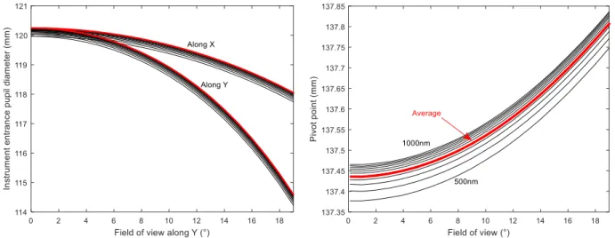
The alignment principle consists in illuminating the instrument with a collimated beam and to measure the spot size. The focal plane position is then varied to search for the best focus. The RMS spot diameter is chosen as a merit function, by definition the best focus is defined as the plane which minimizes that function. The instrument is designed to work at an operation temperature of -80°C. However, the alignment is performed at the ambient temperature of the clean room which is between 18 and 20°C.The instrument is thus aligned in conditions where the optical and mechanical elements are under a thermal configuration which is different from operation conditions. As a consequence, the best focal plane is displaced and the spot size at ambient best focus is increased to reach an RMS diameter of about 90 µm. This means that when the alignment is performed at ambient temperature, the FPA is not located at the best focus of the operation conditions. Consequently, a theoretical shift must be applied to move the FPA from best focus at ambient to best focus at -80° before locking the FPA to the telescope. Of course, this requires an excellent knowledge of the thermal behavior. When illuminating the instrument to perform the alignment, the full entrance pupil of the camera must be fully illuminated by the collimated beam. The entrance pupil is a function of the wavelength and of the field of view, a phenomenon known under the name of pupil walking. The ray-tracing software CodeV was used to calculate the entrance pupil diameter, projected in the plane normal to the optical axis. This was performed simply by calculating the distance between the marginal rays along X and along Y. Figure 3-1-left shows the diameter of the beam in the plane normal to optical axis as a function of the field of view, for wavelengths between 500nm and 1000nm with steps of 10nm. Moreover, to center the beam on the entrance pupil it is necessary to calculate the pivot point. The pivot point is defined as the point on optical axis toward which the chief ray points when entering the optical system. By definition, the pivot point distance is calculated with respect to the first optical surface. The pivot point is also a function of the wavelength and field and was calculated with CodeV, its evolution is shown on Figure 3-1-right. As the alignment is done with white light, the beam rotates around the average pivot and must have a beam diameter of about 121mm, to which some margin is taken.

Figure 3-1: (Left) Entrance pupil diameter as a function of the field, estimated in the plane normal to optical axis. (Right) Pivot point calculated from the first optical surface, as a function of the field

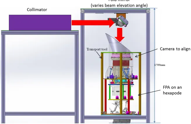
Figure 3-2 shows the setup on which the alignment of the cameras is performed. The instrument is placed on a support assembly with its optical axis pointing vertically; a rotation stage allows rotating the instrument around that axis. A collimator is used to create a collimated beam along the horizontal direction. The beam is then reflected by a fold mirror toward the PLATO camera. The fold mirror is placed on a rotation stage as well as on a translation stage. With this combination of elements, the instrument can be illuminated over the entire field of view: the elevation angle is varied by rotating the fold mirror while the azimuthal angle is varied by rotating the camera around the vertical axis. Moreover, the translation stage of the fold mirror is used to ensure that the collimated beam is always centered on the pivot point. The focal plane assembly is fixed on a hexapod below the instrument. With the hexapod, the FPA position can be varied with 6 degrees of freedom, 3 translations and 3 rotations at micrometer accuracy. Finally, the full setup allows acquiring spot images at the detector for different fields and for different positions/orientations of the FPA, thus enabling to search for the optimal FPA position.

3.2 Alignment methodology

The preliminary step consists in performing a theoretical alignment of the focal plane assembly. Reference cubes are placed on both the instrument and on the focal plane assembly. A theodolite is used to adjust the orientation of the camera with respect to the FPA. The goal is to align the normal of the FPA with the optical axis and the FPA azimuthal angle, within the limit of the reference cubes accuracy. The centering of the FPA relative to the optical axis is made thanks to a laser tracker. Initially, the FPA is placed at the theoretical focus distance of 5.6mm from the last lens, a position which is also verified by laser tracker and which is valid within the accuracy limit of the references on the instrument and on the FPA. A reference frame Л is defined with its (x,y) axis contained in the plane of the FPA and the z axis along the normal direction. The alignment is performed in that reference frame.

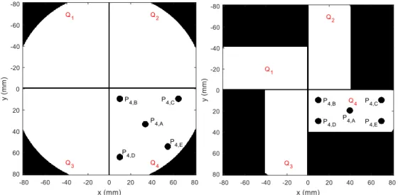
Figure 3-3: Representation for quadrant 4 of the fields that are considered for the alignment process

The next steps of the alignment are based on the measurement of images considering illumination of the instrument at different field positions. A total of 25 fields per camera are defined with 5 per quadrant. Figure 3-3 shows those fields in quadrant 4 for both the normal and fast cameras. Each field is labeled Pq,g where q stands for the quadrant number and

where g goes from A to E and represents different fields inside each quadrant. Coarse measurements are performed with the fields Pq,A to obtain a first estimation of the best focal plane. For each of these fields, images are recorded at the

detector as a function of the focus z in reference frame Л, considering a large step of 200 µm and ranging on several millimeters of scan. Figure 3-4 shows the result of such a scan for a field of 15° obtained with CodeV. As it shows, the RMS spot size increases with a linear behavior when departing from the best focus. A linear fit is performed on both sides of the curves and the intersection between the two lines gives the first coarse estimation of the best focus.

The next step consists in determining accurately the best focus for each of the fields. For that, fine scans are performed around the first approximation z0 of the focus which was determined during the coarse measurements. The initial

imprecision on the estimated best focus is labeled Δz0 and is equal to ±200 µm.

Initial best focus estimation: (1)

The focus position is scanned within that interval by steps of Δz0/2, meaning at a total of 5 distinct positions. At each

position, an image of the spot at the detector is acquired and the RMS spot diameter is calculated.

(2)

The position giving the smallest RMS spot diameter provides a new estimation of the best focus, labeled z1. Provided

that the RMS spot diameter Φ is measured with an accuracy high enough so that this position indeed corresponds to the best focus position within the different scanned positions, the new estimation now has an error of Δz0/2.

(3) (4)

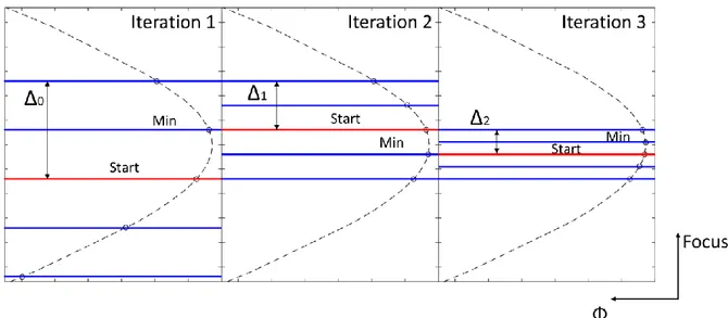
(5) If the error Δz1 is larger than the accuracy with which the focal plane assembly should be aligned, the cycle above is

repeated. Hence, a scan is performed in the interval z1±Δz1 by steps of Δz1/2. This will provide a new estimation of the

best focus z2 with an accuracy Δz2=Δz1/2. The process is repeated iteratively (Figure 3-5), scanning inside zj±Δzj by

steps of Δzj/2 to get an estimated best focus zj+1 with accuracy Δzj+1=Δzj/2. Once Δzj+1 is smaller than the target

alignment accuracy, the process is stopped.

More generally, the process described above can be done by scanning the focus with 2N+1 steps of Δzj/N at each

iteration with any N≥2. At each iteration, the error is reduced by a factor N and thus the error evolves with the iteration number j as 1/Nj _{(equation 6). This allows to directly determine the number of iterations required to decrease the error}

from Δz0 to Δzj. (equation 7). For example, if we want to get an accuracy Δzj=5 and if Δzj=200µm, equation 7 with N=2

gives j=5.3 and thus 6 iterations are enough to reach the alignment accuracy. Let’s also remark that selecting a large value for N is not necessarily interesting as while it will decrease the required number of iterations, it will increase the number of measurements per iteration.

(6)

(7)

The fine alignment process is performed for each of the 5 fields in each of the 4 quadrants. Moreover, the centroid of the spot at the best focus for each field is calculated. Hence, at the end of that process, each field is associated to a set of points (xqg, yqg, zqg), where zqg is the best focal plane distance and (xqg, yqg) is the lateral position of the spot in that plane.

A reference frame Л* is defined based on that plane. Its axis (x,y) are defined inside the plane to have symmetrical azimuthal angles for the different set of fields. The z axis points normal to the plane. The origin of the axis is located at the centroid of the different points (xqg, yqg, zqg). Next, the rotation and translation matrix to pass from Л to Л* is

calculated and that operation is applied to the focal plane assembly with the hexapod. The focus position is then adjusted to position the FPA at the weighted average focus position for all fields. Finally, the lateral position of the spot associated to the different fields is calculated and a fine adjustment of the lateral position of the FPA is performed to center the fields on the different quadrants.

3.3 Dithering to enhance the alignment accuracy

When an image of the spot is recorded with the focal plane assembly located close to the best focus, the spot diameter is close to the size of a pixel. For example, for a field of 15° the RMS spot size is about 90 µm diameter, which represents only 5 pixels. Hence, close to focus the spot size is sampled on a small number of pixels and the calculated RMS spot size become very sensitive to the centering of the spot with respect to the detector array. When measuring the RMS spot diameter as a function of the focus position, this means that the curve presents a large error bar in the area close to best focus. Consequently, it is not possible to distinguish the smallest RMS diameter when comparing the spot at two focus distances which are as close to each other as 5µm.

The solution to this problem is to use dithering to increase artificially the sampling rate. Indeed, such an increase of the sampling rate would make the RMS spot diameter calculation less sensitive to the centering of the spot with respect to the detector array. Hence, the spot diameter versus defocus would have a lower error bar [4]. To do so, the method consists in performing a lateral scan of the focal plane assembly along X and Y by steps of pix/Ndit. At each lateral

position, an image is acquired at the detector. Each of the Ndit² images can then be recombined to form an artificially

high resolution acquisition. Figure 3-6 shows an example of a spot which has been acquired with a different value for the dithering parameter. When Ndit=1, the image is acquired with no dithering and the sampling of the spot is very clear.

When Ndit is increased, the figure shows a very significant improvement of the spot sampling.

N

=1

N

=3

N

=6

N

=9

Figure 3-6: Example of a spot acquired at detector with different values of the dithering (log scale)

Figure 3-7 shows examples of measurement of the RMS spot diameter as a function of the defocus, obtained with CodeV at a field of 15° considering a dithering with either Ndit=1 (left) or Ndit=3 (right). For each focus position, the spot was

acquired at the detector considering the respective dithering parameter and the RMS spot diameter was calculated. This operation was repeated in Monte Carlo simulations by changing slightly the centering of the spot with respect to the detector array. The average RMS spot diameter was then computed as well as the standard deviation. On Figure 3-7, the curves show the average value of the RMS spot diameter and the error bar is the standard deviation. As it shows, the error bar is very large for Ndit = 1, which makes it impossible to distinguish the best focus within several tens of microns.

However, in the case where the dithering is used with Ndit = 3, the error bar is significantly reduced and it is possible to

distinguish the best focus with an enhanced accuracy. The larger the dithering Ndit, the smaller the error on the

measurement spot diameter.

N

=1

N

=3

The set of equations below shows how the dithering is performed mathematically. Assuming a given value for the dithering parameter Ndit, the lateral scanning displaces the focal plane assembly by (dxk, dyk) as defined in equations 8.

By definition, Sij,k1,k2 is the signal acquired at pixel (i,j) when the focal planed assembly is shifted by (dxk1, dyk2). Hence,

the spot reconstructed with images acquired with dithering has a centroid (xc,yc) which can be computed directly with

equations (9). The resulting values are then used in equation (10) to compute the RMS spot size.

with (8)

(9)

(10)

Using dithering improves significantly the accuracy of the measured spot diameter. However, this is at the expense of an increase of the number of measurements to be performed. Moreover, this increase is quadratic with the dithering parameter Ndit. Hence, it is necessary to select Ndit large enough to be able to perform the alignment with the required

accuracy, however Ndit should be as small as possible to limit the measurement time. The question is thus: how to choose

the value of Ndit?

We consider two focus positions spaced by dz and giving a variation of the RMS spot diameter dΦ (Figure 3-8). The dithering should be adjusted so that the error on the measured spot diameter is small enough so that we can distinguish which of the two focus positions gives the smallest RMS spot diameter. Equation 11 is the proposed criteria, where σΦ

represents the standard deviation of the RMS spot diameter due to the sampling on the detector array. With such a criterion the measured spot diameter will have an error below dΦ/2 at 2sigma probability (95%).

(11)

In the fine alignment process, the criteria of equation 11 translates into equation 12, were dΦ is evaluated based on a defocus Δzj/N. At each iteration, the scan step is decreased by a factor N. Thus, the difference of RMS spot diameter to

distinguish is smaller and the requirement on the error σΦ becomes more stringent. Hence, the dithering parameter Ndit

should be adapted to the minimum value which provides an error σΦ which fulfills equation 12 at the iteration which is

considered.

(12) CodeV simulations were used to provide the requirement with equation 12 and to determine the relation between the dithering parameter Ndit and the error σΦ. If we first consider focus positions located on the same side of the spot size VS

focus curve, the worst case for dΦ[Δzj/N] occurs when one of the point is located precisely at best focus. Indeed, this is

when the defocus Δzj/N will provide the smallest variation dΦ. In the case where the points were not on the same side,

the variation dΦ would be even smaller and could even reach 0. This is however not an issue as even if we are not able to distinguish which of the two points have the smallest spot diameter, whichever is selected then the best focus will be included inside the scanning zone at the next iteration.

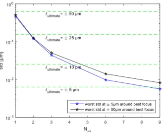
Figure 3-9 shows the error σΦ as a function of the dithering parameter Ndit, obtained with CodeV simulations at a field of

15°. It shows as expected that the error decreases when Ndit increases. The horizontal dotted lines corresponds to the

maximum error to fulfill the criteria of equation 11, considering different values of dz. For that, the relation between dΦ and dz was computed with CodeV in the most constraining assumption where one point is located at best focus. From this curve, we can directly see what is the minimum value of Ndit which provides an error σΦ small enough to fulfill the

criteria of equation 11.

Figure 3-9: Error on the RMS spot diameter, σΦ, due to the sampling by the detector array as a function of the dithering

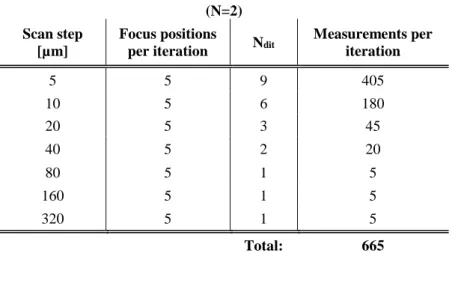
Table 1 below shows how the dithering evolves with the alignment iterations when considering N=2. Moreover, it shows how many measurements are necessary to reach the required alignment accuracy. As it shows, the first iterations don’t require any dithering. When the scanning step becomes as small as 40 microns, a dithering of 2 is required and when the step reaches 5 microns the dithering goes up to 9. The total number of measurements per iteration thus increases significantly when the scan steps decreases due to the quadratic dependence on the dithering parameter. When starting from an initial scanning step of for example 320µm, a total of 665 measurements are required where the two third of the measurements are performed at the last iteration. Remark also that the first iterations require the less measurement, thus it doesn’t affect significantly the total number of measurements if the first estimation of the best focus is known with an accuracy of 320µm or even twice that value.

Table 1. Evolution of the dithering as a function of the scan step, number of measurements per iterations and total number of measurements.

(N=2) Scan step

[µm]

Focus positions

per iteration Ndit

Measurements per iteration 5 5 9 405 10 5 6 180 20 5 3 45 40 5 2 20 80 5 1 5 160 5 1 5 320 5 1 5 Total: 665

4. CONCLUSIONS

An automatized method has been developed to align the focal plane assembly on the 26 cameras of the PLATO mission. The principle of the alignment is to illuminate the camera with a collimated beam and to vary the position of the FPA to search for the position which minimizes the RMS spot diameter. The first step of the alignment is done theoretically based on references on the instrument and on the FPA and involves the use of a theodolite and of a laser tracker. The fine alignment is done by iteratively searching for the best focus, decreasing at each step the error on the estimated best focus by a factor 2. In the conditions of PLATO and in absence of measurement noise, 6 iterations only are required to reach the desired accuracy. Due to the sampling of the detector, the measured RMS diameter measured on a single acquisition of a spot is affected by a large inaccuracy. Indeed, the RMS spot diameter is very sensitive to the lateral centering of the spot with respect to the detector array. If nothing was done, the alignment could not be performed with less than several tens of microns accuracy. The solution to this issue is to use dithering to increase the spatial sampling of the spot and desensitize the RMS spot diameter from the centering on the detector array. This is performed with a series of in-plane scans. It was shown that it reduces the error on the RMS diameter significantly, thus enabling an alignment with an enhanced accuracy. The drawback of the dithering process is that it increases the number of measurements to perform and thus it increases the time needed for the alignment. A criterion was proposed to determine the optimal dithering parameter to select when considering a given scan range. Hence, at each iteration the scanning step is decreased and the dithering parameter is increased. It was shown that a total of about 665 measurements need to be performed to converge to the best focus with an accuracy of 5µm, starting from an initial error of 320µm. These results don’t consider the noise at the detector, which will be a source of error on the spot diameter and will be included in a next step of the alignment process optimization.

REFERENCES

[1] Ragazzoni, R. et al., "PLATO: a multiple telescope spacecraft for exo-planets hunting", Proc. SPIE 9904, Space Telescopes and Instrumentation 2016: Optical, Infrared, and Millimeter Wave, 990428 (29 July 2016)

[2] Magrin, D., Munari, M., Pagano, I., Piazza, D., Ragazzoni, R., Arcidiacono, C., Basso, S., Dima, M., Farinato, J., Gambicorti, L., Gentile, G., Ghigo, M., Pace, E., Piotto, G., Scuderi, S., Viotto, V., Zima, W., Catala, C., "PLATO: detailed design of the telescope optical units", Proc. SPIE 7731, Space Telescopes and Instrumentation 2010: Optical, Infrared, and Millimeter Wave, 773124 (5 August 2010)

[3] Laubier, D., Bodin, P., Pasquier, H., Fredon, S., Levacher, P., Vola; P., Buey, T., Bernardi, P., "The PLATO camera", Proc. SPIE 10564, International Conference on Space Optics — ICSO 2012, 1056405 (20 November 2017)

[4] Jomni, C., Ealet, A., Gillard, W., Prieto, E., Grupp, F., "On-ground tests of the NISP infrared spectrometer instrument for Euclid", SPIE 10562, International Conference on Space Optics — ICSO 2016, 105625M (25 September 2017)