Unique parameter identification for cardiac diagnosis in critical care using
minimal data sets
C.E. Hanna, , J. G. Chasea, T. Desaiveb, CF. Froissartc, J. Reviea, D. Steυensona, B. lambermontb, A. Ghuysenb, P. Kolhb, CM. Shawd
a Department of Mechanical Engineering, Centre for Bio-Engineering, Private Bag 4800, University of Canterbury, Christchurch 8020, New Zealand
b
Hemodynamics Research Laboratory, University of liege, Belgium c Université de Technologie de Belfort-Montbéliard, France
d Department of Intensive Care, Christchurch Hospital, Christchurch, New Zealand
Abstract
Lumped parameter approaches for modelling the cardiovascular system typically have many parameters of which a significant percentage are often not identifiable from limited data sets. Hence, significant parts of the model are required to be simulated with little overall effect on the accuracy of data fitting, as well as dramatically increasing the complexity of parameter identification. This separates sub-structures of more complex cardiovascular system models to create uniquely identifiable simplified models that are one to one with the measurements. In addition, a new concept of parameter identification is presented where the changes in the parameters are treated as an actuation force into a feed back control system, and the reference output is taken to be steady state values of measured volume and pressure. The major advantage of the method is that when it converges, it must be at the global minimum so that the solution that best fits the data is always found.
By utilizing continuous information from the arterial/pulmonary pressure waveforms and the end-diastolic time, it is shown that potentially, the ventricle volume is not required in the data set, which was a requirement in earlier published work. The simplified models can also act as a bridge to identifying more sophisticated cardiac models, by providing an initial set of patient specific parameters that can reveal trends and interactions in the data over time. The goal is to apply the simplified models to retrospective data on groups of patients to help characterize population trends or un-modelled dynamics within known bounds. These trends can assist in improved prediction of patient responses to cardiac disturbance and therapy intervention with potentially smaller and less invasive data sets. In this way a more complex model that takes into account individual patient variation can be developed, and applied to the improvement of cardiovascular management in critical care.
Keywords : Model-based cardiac diagnosis ; Cardiovascular system ; Integral-based parameter identification ;
Pressure waveform ; ECG ; Intensive care unit
1. Introduction
In critical care, cardiovascular dysfunction can be easily misdiagnosed due to incomplete information and the complexities involved, leading to premature discharge or non-optimal treatment [1-3]. It is also a major cause of increased length of stay and death [4,5]. Demand for critical care is growing dramatically severely affecting healthcare delivery [6-8]. The overall goal of this research is to use computational cardiac models to better aggregate available clinical data in an intensive care unit (ICU) into a more readily understood physiological context for clinicians. The computational models can be used to reveal non-linear dynamics and interactions that are not readily apparent in the data.
A major difficulty faced with cardiovascular modelling in general, is the level of detail these models typically include. For example multi-scale modelling approaches utilizing finite elements have successfully explained complex behaviour of the heart [9-11]. Although this paper does not seek to compare to finite elements in any way, it does represent the extreme case where knowledge of complex geometry of blood vessels (e.g. from an MRI scan) is required as well as many parameters that are not typically available in an ICU setting. Furthermore, the main problem with methods requiring an MRI is related to the cost, since interpretability has become quite standard. Hence the application itself puts a constraint on the models used. For example in an ICU, near real-time feedback (<5 min) is required. Typical finite element models can require hours or days running on a super
computer, which is not always available. Hence a large gap exists between the computational results of these detailed models and real-time clinical utility.
Lumped parameter models (LPM) are a common approach to minimizing complexity in the cardiovascular system [12-16] but there are still many parameters involved. Thus typically, only small subsets of the parameter set can be identified (e.g. [14]), even though the full model is run each time to match patient data. As a result, a majority of the parameter set has to be fixed at population values, so that a significant amount of dynamics in the model may not be reflective of individual patient responses. There also may be significant interaction between the identified small subset and the rest of the model that prevents a consistent characterization of parameters. For example a more complex model would have a significantly different transient response and settling time to steady state. Furthermore, the time to steady state may vary considerably depending on initial conditions, which in critical care are never fully known since a patient's condition can regularly change rapidly. This transient variation would make parameter identification more difficult and less reliable, as well as increasing computational requirements that may limit real-time patient specific application at the bedside.
This paper presents a different approach, by first developing simplified, fully identifiable, patient specific models, that are based around the clinical data available in an ICU. Interactions between identified parameters over time, and for different patients and interventions can be then analyzed to build more complexity into the model as required, to predict observed patient hemodynamic responses. Hence these models essentially act as a bridge to identify complex physiological behaviour in ICU patients. In the simplified models, patient specific dynamics are only considered if they can be uniquely identified from the given data. This modelling constraint, allows any un-modelled dynamics to be consistently characterized over all patients. Due to the simplified structure of these models, it is then possible to analyze the primary geometric effects of given input parameters on the output, thus simplifying parameter identification.
Note that the word identifiability referred to here is "practical identifiability" with respect to noise and modelling error, which can currently only be tested numerically [17,18]. General identifiability theory [19,20] refers to the ideal case of perfect knowledge of the system and measurements, which does not guarantee that parameters can be identified uniquely in practice. Hence, this study views identifiability from the perspective of the final application. Also note that the models developed are only created for purposes of simplifying parameter identification of the full model on retrospective data. The issue of forecasting measurements and responses in the future to guide therapy is not addressed in this paper. This task would likely be more appropriate for a more physiologically complete model and is left for future investigations.
A key goal in this paper is to demonstrate how the main dynamics of a given CVS model can be simply identified from measured retrospective data. A common method of modelling the CVS is by a series of elastic chambers connected by resistors with a time varying elastance. This approach has been well developed and validated in the literature [12-16] so it serves as a good starting point to test the methods and concepts in this paper. The specific baseline model structure considered is a six chamber cardiovascular model including ventricular interaction and inertial effects that has been previously developed [16] and validated in clinical animal trials [21-24]. However, note that the approach is general and could be applied to any cardiac model structure.
A new concept developed in this paper matches simplified CVS model outputs to continuous information of arterial/pulmonary pressures and the end-diastolic time from an ECG or the "a wave" timing from the pulmonary pressure waveform. Adding continuous pressure waveforms and end-diastolic timing to current clinical data sets is shown to increase the diagnostic ability of the model and enable a more minimal data set that does not require maximum and minimum volume measurements. Hence, this approach adds a simple and easy measurement to remove the need for a more invasive, difficult and noisy measurement.
The new methods are rigorously tested in simulation with noise corrupted measurements and modelling error to prove robustness. Finally, animal data is used to demonstrate the clinical potential of these methods.
2. Methodology
2.1. Cardiac model
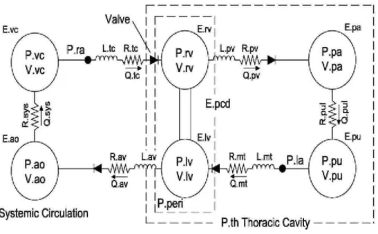
The cardiovascular system model used in this paper consists of six elastic chambers, as shown in Fig. 1. First developed in [16], it has been validated clinically [21-24].
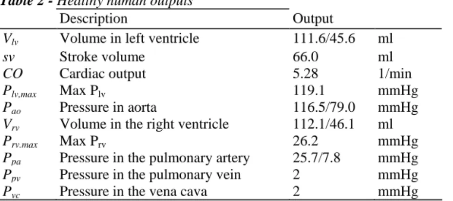
All the input parameters for a healthy human baseline state are defined in Table 1. The output parameters are shown in Table 2 [25].
For simplicity, only the differential equations associated with the left ventricle are shown here, where [16] has a description of the full model.
In Eqs. (l)-(9), the parameter H(t) is the Heaviside function, Qav and Qmt are the flows through the aortic valve
and mitral valve of the left ventricle, Pαo, Ppv and Plv are the pressures in the aorta, pulmonary vein and left
ventricle, Vlv is the volume in the left ventricle, Vspt is the septum volume and Pperi is the pressure in the
pericardium. The Heaviside formulation of Eqs. (1) and (2) provides an open on pressure close on flow valve law such that:
where Eq. (10) holds during ejection and Eq. (11) during filling. Ventricular interaction is included by modelling the septum volume Vspt by the following equation [16]:
Note that, Eq. (12) is derived by setting the septum pressure volume relationship equal to the difference between the left and right ventricle pressures, for more details see [16]. Eq. (12) is solved for Vspt at each time step using a
Fig. 1 - Six chamber CVS model with inertial effects and ventricular interaction.
Table 1 - Healthy human parameters
Parameters Values Units
Eao Elastance of aorta 0.6913 Hg/ml
Rav Resistance of aortic valve 0.0180 mmHg.s/ml
Lav Inertance of aortic valve 1.2189E-004 mmHg.s2/ml
Ees,lvf Elastance of left ventricle 2.8798 Hg/ml
Rmt Resistance of mitral valve 0.0158 mmHg.s/ml
Lmt Inertance of mitral valve 7.6968E-005 mmHg.s2/ml
Rsys Systemic flow resistance 1.0889 mmHg.s/ml
Epa Elastance of pulmonary artery 0.3690 Hg/ml
Epu Elastance of pulmonary vein 0.0073 Hg/ml
Ees,rvf Elastance of right ventricle 0.5850 Hg/ml
EVC Elastance of vena cava 0.0059 Hg/ml
Rtc Resistance of tricuspid valve 0.0237 mmHg.s/ml
Rpuv Resistance of pulmonary valve 0.0055 mmHg.s/ml
Rpul Pulmonary flow resistance 0.1552 mmHg.s/ml
Ees.spt Elastance of the septum 48.7540 Hg/ml
Additional parameters
Period Time of one heart beat 0.75 s
P0.luf Defines gradient of EDPVR at 0 pressure 0.1203 mmHg
P0.rvf Defines gradient of EDPVR at 0 pressure 0.2157 mmHg
P0.pcd Pressure in pericardium at 0 volume 0.5003 mmHg
P0.spt Pressure in RV at 0 septum volume 1.1101 mmHg
Pth Pressure in the thoracic cavity -4 mmHg
λlυf Parameter of the EDPVR 0.033 1/ml
λrvf Parameter of the EDPVR 0.023 1/ml
λspt Parameter of ventricular interaction (VI) 0.435 1/ml
λpcd Parameter of VI 0.03 1/ml
V0.spt Parameter of VI 2 ml
Table 2 - Healthy human outputs
Description Output
Vlv Volume in left ventricle 111.6/45.6 ml
sv Stroke volume 66.0 ml
CO Cardiac output 5.28 1/min
Plv,max Max Plv 119.1 mmHg
Pao Pressure in aorta 116.5/79.0 mmHg
Vrv Volume in the right ventricle 112.1/46.1 ml
Prv.max Max Prv 26.2 mmHg
Ppa Pressure in the pulmonary artery 25.7/7.8 mmHg
Ppv Pressure in the pulmonary vein 2 mmHg
Pvc Pressure in the vena cava 2 mmHg
Fig. 2 - (a) The left ventricle-systemic system simplified model, (b) The right ventricle-pulmonary system
simplified model.
2.2. Simplified model
Simulation has shown that the pressure in the pulmonary vein Ppv, and the pressure in the vena cava Pvc, typically
vary in this model by only approximately 0.5mmHg over a cardiac cycle [26]. Thus, Ppv and Pvc are essentially
close to constant. If Ppv and Pvc are held constant for the model of Fig. 1, and ventricular interaction Vspt and the
pressure in the pericardium Ppcd are set to zero, both the left and right systems of the CVS can be separated.
However, note that the stroke volumes of the left and right ventricles would be the same in the measured data. Therefore, since the identification algorithm would match the left and right ventricle models to this data, there still remains an inherent coupling between the systems.
The assumptions of Vspt = 0, and Ppcd = 0, are made primarily as an initial mathematical simplification to the
model and to introduce modelling error to test the robustness of the derived methods. In all cases, the "measured data" used in this paper, includes both ventricular interaction and pericardium dynamics. Physiologically, the pressure in the pericardium Ppcd is typically close to zero, but can increase significantly with pericarditis,
although it still only contributes up to about 25% of left ventricular pressure [27,28]. Ventricular interaction can have significant effects on the right ventricle, but has less of an effect on the left ventricle [29].
Significant simulation studies have shown that changes in the inertances Lmt and Lav in Fig. 1 and Eqs. (1) and (2)
do not significantly effect parameter identification [26]. The parameter Po.iu/ has also been shown to have a limited effect [26] and for discrete data is typically identified to be close to 0 [21]. Therefore Lmt, Lav and P0,lυfare
set to 0. The resulting two models are shown in Fig. 2, where the direction of the left ventricle-systemic system has been reversed from Fig. 1 to illustrate the similarities.
Replacing the input/output parameters:
in the left ventricle-systemic system of Fig. 2(a) with the parameters:
the right ventricle-pulmonary model of Fig. 2(b) is obtained.
A final addition is to create an extended driver function e(t) to reduce the modelling error caused by the above simplified model assumptions. The new driver function and the model differential equations for the left ventricle-systemic system of Fig. 2(a) are defined.
The left ventricle-systemic system of Fig. 2 (a) can be modelled:
where Ppv and Pvc are held constant. The parameters Plv,full and Vlv,full are defined to be the full model outputs of
Fig. 1 from a healthy human parameter set with a heart beat period of 0.75 s. Hence Eq. (20) represents a population driver function, which could be scaled to represent different heart beats. However, the shape could be altered as required to capture individual patients. To obtain the model equations for the right ventricle-pulmonary system of Fig. 2(b), the parameters of Eq. (13) in Eqs. (15)-(20) are replaced by the parameters of Eq. (14). 2.3. Healthy and disease state comparisons
To model a diseased human, the following set of parameter changes are made from Table 1:
The changes in Eq. (21) are used as an initial mathematical validation of the simplified models in Fig. 2, rather than a physiologically realistic study of the clinical mechanisms involved in cardiac dysfunction. However, a halving of contractility Ees,lvf and systemic resistance Rsys is not too unrealistic for septic shock, or myocardium
increase in the resistances of the aortic and mitral valves [30,32,33]. The disease states in Eq. (21) would of course be unlikely to occur all at once, but it serves to provide an initial test of the methods.
2.4. Unique parameter identification
The parameter identification method presented is an extension of the concept developed in [21,26]. The idea in [21,26] is to set up an iteration between a linear least squares optimization and a forward solution, which is partly based on a Picard iteration [34]. This approach is therefore distinctively different from other integral formulations like the modulating function approach [35] which does not iterate and is therefore not directly suitable for the discrete data and high non-linearities present in this application. Furthermore, the CVS model of Fig. 1 typically requires many iterations to converge to steady state, which is highly dependent on the initial conditions. Therefore, the standard method of non-linear regression [36], is not suitable, as it is too computationally intense and can often result in local minima. In this section the method of [21] is significantly improved by avoiding the requirement of a continuous volume profile, which is typically not known. In addition the number of forward simulations and the computational requirements for each iteration are dramatically reduced.
The unknown patient specific parameters, denoted X, that are optimized for the left ventricle are defined:
The parameter Pvc in Eq. (13) is assumed known, since it would be found from either identifying the right
ventricle system, or by direct measurement of the central venous pressure, which is common in an intensive care unit.
There are six unknown parameters in Eq. (22) to be identified in the model of Fig. 2(a). Therefore, the measured maximum/minimum left ventricle volume and aortic pressure can only uniquely identify four of these parameters. However, the timing of the mitral valve closure corresponds to the end of the atrial contraction which can be detected by the end of the P wave on an electrocardiogram (ECG) [25]. Alternatively, since the left and right atriums contract close to simultaneously, the mitral valve closure can also be calculated from the "a wave" in the central venous pressure waveform [37]. The central venous pressure is commonly measured in the ICU.
These observations demonstrate an important concept, which is to utilize features from physiological waveforms to improve identifiability without having to explicitly model the effects. The pressure in the pulmonary vein Ppv
or the filling pressure of the simplified model of Fig. 1(a) corresponds to the left ventricle pressure at the mitral valve closure. Hence, Ppv can be estimated by the formula:
A further important feature available is the maximum gradient or inflection point in the ascending aortic pressure wave. The parameter which has a significant effect on the maximum aortic pressure gradient is the resistance in the aortic valve Rav. Define:
where Pao,approx and Pao,true are the simulated and "measured" aortic pressures, tmin is the time of minimum aortic
pressure and tinflect is the time of maximum aortic pressure gradient. Eq. (24) is an approximation to the ratio of
the maximum gradients of Pao,approx to Pao,true and is used to avoid having to differentiate the aortic pressure
which may be noisy. Simulation has shown that the variable α in Eq. (24), changes inversely proportional to Rav
with all other parameters held at their nominal values. Specifically, if Rav increases by a factor of 2, with all other
parameters fixed, α approximately reduces by a factor of 2, with a order of magnitude less effect on the maximum and minimum volumes/pressures. This result motivates an approximation to Rav:
However, for Eqs. (23) and (25) to be valid approximations, to Ppv and Rav, the approximations Plv,approx and
Pao,approx need to be as accurate as possible. The solution proposed, is to first ensure that the maximum/minimum
simulated volumes and aortic pressures are precisely matched to the measured values for given initial (but essentially arbitrary) estimates of Ppv and Rav. At the end of this optimization, Ppv and Rav are updated using Eqs.
(23) and (25).
Simulation has shown that increasing the parameters Ees,lvf, and Rmt separately by factors of 2 decrease the mean
volume, and stroke volume by factors close to 2. On the other hand, increasing the parameters for Eao and Rsys
proportionally increase the pulse pressure difference and the mean aortic pressure. These results motivate the following definitions:
Consider Rmt,approx in Eq. (27). Integrating Eq. (17) over one heart beat yields:
For a given Ppv, let be the current estimate of Rmt,true, with corresponding approximations and to Plv,true
and SVtrue· Therefore:
Assuming that is much closer to Plv,true than is to SVtrue it follows that:
Therefore, Eq. (27) also follows from an integral formulation of Eq. (17) over one heart beat period. A similar approach (not shown) can be used to derive Eqs. (26), (28) and (29).
Note that an alternative approach would be to scale the approximate waveform so that then evaluate the ratio of the integrals in Eq. (32). However, evaluating Eq. (32) directly, which is effectively the method of [21], relies on approximating the continuous left ventricle waveform Vlv throughout the heart beat,
which can introduce errors. In prior work [21], the estimates and the accuracy of convergence often relied on reasonable starting waveform shapes, and in some cases did not converge satisfactorily without some manual
intervention. The method of Eqs. (26)-(29) only requires discrete data and is similar to proportional feedback control. That is, these parameters can be considered to be the actuation force that controls the reference output, which is the measured volumes and pressures. The only difference is that instead of applying a force proportional to the difference between the reference and actual output, the force is proportional to the ratio of the reference to actual output. Specifically, the parameters in Eqs. (26)-(29) continually change until the ratios are driven to one and is thus fully automatic.
Fig. 3 - Parameter identification algorithm for Fig. 2(a).
Step 1 Choose arbitrary set of input parameters including Ppv and Rav
Step 2 Simulate model of Equations (15)-(20)
Step 3 Compute approximations to Es,lvf, Rmt, Eao and Rsys from Equations (25)-(28).
Step 4 Simulate model of Equations (15)-(20).
Step 5 If the maximum volumes and aortic pressures are matched within a given tolerance to data in Equation
(34), go to Step 6, otherwise go back to Step 3.
Step 6 Compute Ppv and Rav from Equations (23) and (25), If they have changed by less than 1% go to Step 7
otherwise go back to Step 3.
Step 7 Output final solution and identified parameters
The method presented is also readily generalizable to parameter identification of other models, by locating the major geometric effects of each parameter on the measured data, and formulating a control system like Eqs. (26)-(29), to iterate the parameters. The specific equations that enable the parameters to converge are of course model specific, but the overall approach and concept, including the breaking down of complex models into sub-models that are fully identifiable, is general.
The tests for the parameter identification method are done first in simulation with noise, and then on animal data. In the tests with noise, the "measured data" is taken to be the output of the six chamber model of Fig. 1. For the animal experiments, the measured data is from catheters [38]. In both cases:
where
The overall parameter identification method is summarized in Fig. 3. Note that there is an outer control loop in step 6, which involves updating Rav from Eq. (25). No control system updates Ppv since it is determined directly
from the left ventricle pressure wave form at the end of the inner loop step. This outer loop for Rav,αpprox behaves
similarly to the inner loop governed by Eqs. (26)-(29), with the constant in front of Rav,old in Eq. (25) approaching
unity as the iterations proceed. When the constant falls between 0.99 and 1.01, the optimization is stopped, which corresponds to Rav,αpprox changing by less than 1%.
Step 1: Choose arbitrary set of input parameters includingPpv and Rav.
Step 2: Simulate model of Eqs. (15)-(20).
Step 3: Compute approximations to Ees,lvf, Rmt, Eao and Rsys from Eqs. (25)-(28).
Step 4: Simulate model of Eqs. (15)-(20).
Step 5: If the maximum volumes and aortic pressures are matched within a given tolerance to data in Eq. (34), go to Step 6, otherwise go back to Step 3.
Step 6: Compute Ppv and Rav from Eqs. (23) and (25). If they have changed by less than 1% go to Step 7
otherwise go back to Step 3.
Step 7: Output final solution and identified parameters.
2.5. No volume measurement
The algorithm of Fig. 3 can be readily extended to the case where the mean Vlv in Eq. (34) is removed. The
method is to let the mean Vlv be an extra unknown parameter and optimized along with the parameters in Eq.
(22). To account for the change in unknown parameters, more information from the aortic pressure waveform is used. Define:
where tmin and tinflect are from Eq. (25), and n is on the sampling frequency of the aortic pressure catheter which is
taken to be 1kHz. The metric error is dependent on the mean Vlv and the points t1 and tn are equally spaced about
tinflect. It is important to note that the full aortic pressure waveform cannot be used in Eq. (36). The reason is that
the model does not capture the dicrotic notch so matching to this part of the waveform would introduce unnecessary error into the method. However, the continuous waveform in the interval [t1, tn] still provides
significantly extra data that can be used to identify the mean volume and thus the maximum/minimum left ventricle volumes as well.
The method starts with an approximation Vlv,max,approx to the maximum volume. The approximate mean volume is
thus defined:
The algorithm of Fig. 3 is then applied and the error in Eq. (36) is computed. The maximum volume Vlv,max,approx
is then updated in a depth first search to minimize the error of Eq. (36). The method is summarized in Fig. 4. Step 1: Choose a value of Vlv,max,approx, and determine the mean Vlv from Eq. (38).
Step 2: Apply the method of Fig. 3 to identify Ppv, Rav, Ees,lvf, Rmt, Eao and Rsys.
Step 3: Compute the error of Eq. (36).
Step 4: Repeat Steps 1-3 in a depth first search until Vlv,max,approx changes by less than a tolerance
percentage. Step 5: Output the final approximation Vlv,max,approx and identified parameters.
Fig. 4 - Parameter identification algorithm for Fig. 2(a) without a volume measurement, but a known stroke
volume.
Step 1 Choose a value of Vlv,approx,max and determine the mean Viv from Equation (38).
Step 2 Apply the method of Figure 3 to identify Ppv, Rav, Ees,lvf, Rmt, Eao and Rsys
Step 3 Compute the error of Equation (36).
Step 4 Repeat Steps 1-3 in a depth first search until Vlv,approx,max changes by less than a tolerance percentage.
3. Results and discussion
This section first validates the simplified modelling approach of Figs. 2(a) and (b), and the parameters identification method of Fig. 3, against simulated data from the full model of Fig. 1. Measurement noise is simulated by corrupting the simulated data with random uniformly distributed noise. Due to the symmetry of Figs. 2(a) and (b) only tests on the left ventricle system are considered. The noise is defined:
where for the end-diastolic filling time td2 in Eq. (34), the 10% noise is relative to the length of time of the
diastole. The noise is made less for the pressure, since it is assumed that a catheter measures the aortic pressure waveform, which is standard in an ICU. Modelling error is also present in the simplified models of Fig. 2 with respect to the full model of Fig. 1. The model and methods of the left ventricle-systemic system are then tested on clinical data from a pulmonary embolism animal model experiment [39].
3.1. Convergence of algorithm and effectiveness of modelling approach
To demonstrate the fast and accurate convergence of the algorithm of Fig. 3, and to assess the suitability of the simplified models of Fig. 2 in describing the full model of Fig. 1, a healthy human is first considered. The parameters for a healthy human are given in Tables 1 and 2. In this case no noise is added so an accurate characterization of the accuracy of the simplified models can be obtained. The assumed measured data is:
where Pao is given as a function of time since it is continuously measured.
The left ventricle volume matches very closely to the true volume with maximum errors of 1.6% and 2.6% during filling and ejection, and errors of 0.00016% and 0.00014% in the maximum and minimum volumes respectively. Similarly, the identified aortic pressure closely captures the true pressure with maximum errors of 1.8% and 0.2% during ejection and filling, and errors of 0.0026% and 0.0015% in the maximum and minimum aortic pressures, respectively. The error in the maximum ventricle pressure is 2.1%.
For the identified parameters, the largest error is 21.7% in Rav but this is largely due to the already small value.
There is also an error of 8.1% in Ees,lvf which reflects the modelling error of Fig. 2 with respect to Fig. 1. These
results show that the simplified model of Eqs. (15)-(20) is a very accurate representation of the full model of Fig. 1, with small errors due to modelling error.
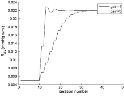
The accurate results also provide an initial validation of the parameter identification method of Fig 3, with very fast convergence obtained, even when starting significantly far away from the solution. Fig. 5 plots the maximum volume and Fig. 6 plots Rav against the number of iterations, for an initial guess containing 300-400%
error in all the parameters. One iteration is equivalent to one numerical simulation of Eqs. (15)-(20) that occurs in Step 3 of Fig. 3. The maximum volume converges in about 10 iterations, and remains largely unaffected by changes
in Rav, where Rav takes about 24 iterations to converge within 1%. The convergence time of Rav can be reduced
by a factor of 2 by re-defining Rav in Eq. (25) by:
and setting a gain of 3, as shown in Fig. 6. Importantly, once the method converges, this implies that the ratios in Eqs. (26)-(29) must be unity, otherwise the parameters would keep changing. Hence, the method can never reach a local minima and must always stop at the global minimum.
Similarly accurate results are obtained for the diseased state human of Eq. (21), so these results are not shown. In summary the parameter identification method of Fig. 3 is very fast and accurate independent of starting point, and the simplified models of Fig. 2 closely capture the full model dynamics of Fig. 1. Importantly, the data of Eq. (34) is sufficient to uniquely identify all six parameters in Eq. (22). The simpler nature of Fig. 2 also means the model simulations are dramatically faster.
Fig. 5 - Convergence of the maximum volume using algorithm of Fig. 3.
3.2. Healthy and diseased human with noise—no volume measurement
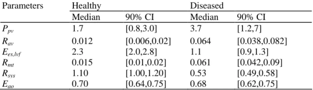
100 Monte Carlo simulations are performed on each of the healthy and disease states, using the algorithm of Fig. 4 with noise levels defined in Eq. (39). To optimize accuracy, a cubic smoothing spline is performed on the noisy aortic pressure waveform using standard in-built functions in Matlab. The result is 100 pairs of identified parameters, which are summarized in Table 3.
The median ratios of Ees,lvf,disease/Ees,lvfheαlthy, Rav, disease/ Rav,healthy, Rmt,disease/Rmt,healthy, and Rsys,disease/Rsys,healthy are 0.48.
5.3, 4.1 and 0.48, respectively, which capture the reduced contractility, increased resistances and reduced systemic resistances as defined in Eq. (20). There are also good separations in the 90% CI's. Note that for Rav and Rmt in Table 3, 90% Of all ratios Rav.disease/Rav.healthy and Rmt,disease/Rmt.healthy Were identified to be greater than
a factor of 3 showing the method is effective at identifying the simulated stenosis for both the mitral and aortic valves. In addition, 90% of the identified maximum volumes have an error less than 11.5% and 14.7% for the diseased and healthy human respectively. However, part of this error is due to the overestimation of the volume in each case. Taking the identified volumes with no noise as the "true" volumes gives 90% of all errors less than 8.7% and 12.2% respectively. Furthermore, 90% of the identified maximum left ventricle pressures have an error less than 1.5% and 9.4%, for the healthy and disease states.
Table 3 - Comparing the identified parameters for a healthy and diseased human with noise from Eq. (39)
Parameters Healthy Diseased
Median 90% CI Median 90% CI Ppv 1.7 [0.8,3.0] 3.7 [1.2,7] Rav 0.012 [0.006,0.02] 0.064 [0.038,0.082] Ees,lvf 2.3 [2.0,2.8] 1.1 [0.9,1.3] Rmt 0.015 [0.01,0.02] 0.061 [0.042,0.09] Rsys 1.10 [1.00,1.20] 0.53 [0.49,0.58] Eao 0.70 [0.64,0.75] 0.68 [0.62,0.75]
Fig. 6 - Convergence of Raυ in the algorithm of Fig. 3 using two gains of 1 and 3 in Eq. (41).
3.3. Further validation on an animal model and clinical implementation
Currently no human data is available to test the methods. Thus, to demonstrate the clinical potential for the methods developed, data from a porcine pulmonary embolism experiment is used. The main purpose of this exercise, is to show that the methods work for different driver functions and with data where there is the potential for significantly greater modelling error that cannot be represented by the six chamber model and noise. The data is obtained from the Hemodynamics Research Laboratory, University of Liege, Belgium. In the experiments, a pig is injected with autologous blood clots every 2 h to simulate pulmonary embolism [38]. As a simple proof of concept, the left ventricle model of Fig. 1(a) and the method of Fig. 2 are applied using measured waveforms for one of the pigs at two time points of 30 min and 210 min. No ECG or the central venous pressure waveform was available, therefore, the end-diastolic filling time td2 in Eq. (34) was manually
estimated from the left ventricle volume profile. A driver function is derived in a similar way to Eq. (20), but with Plv,full and Vlv,fullreplaced by the measured left ventricle pressure and volume, and Pth is set to 0, since the pig
is open chest. The resulting function is smoothed by least squares cubic splines and normalized so the maximum point is 1 and the time interval of one heart beat is the healthy value of 0.75. To account for different heart rates, the generic shape is defined:
where is experimentally derived from the healthy state of several pigs based on an average response and is shown in Fig. 7.
To account for individual pig variations the final driver function is defined:
where tao,min is the time of minimum aortic pressure, is the time of the minimum (or maximum negative)
Specifically, is well known to correspond to the minimum left ventricle pressure gradient (or inflection point) which always occurs just before the dicrotic notch, and thus corresponds to the aortic valve closure. The volume is approximately constant at this point, and therefore, the formula of Eq. (20) shows that tinflect,2 should
be equal to . The maximum left ventricle pressure gradient, is also known to occur justbefore the aortic valve opens, which corresponds closely to tao,min. Therefore since the volume is constant at this point as well,
tinflect,1 should be equal to tao,min. The time scaling transformation in Eq. (43) ensures that the inflection points of
the driver function correspond to tao,min and as required. Eqs. (42) and (43) therefore provide a way of
approximately identifying a patient (pig) specific driver function. Further clinical experiments and trials on humans are needed to classify to what degree of accuracy the driver function is required to be for adequate cardiac diagnosis.
Fig. 7 - Experimentally derived driver function n based on Eq. (20).
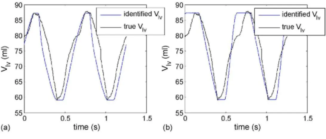
Fig. 8 - Applying the algorithm of Fig. 3 to the pig data, (a) Identifying all parameters, (b) Fixing Ppv and Rav.
3.3.1. Parameter identification with known volumes Fig. 8(a) shows the result of applying the algorithm of Fig. 3 on the one of the pigs at 30 min into the pulmonary embolism experiment. This figure is compared to a special case of a fixed
Ppv = 2 and Rav = 0.46 in Fig. 8(b). In both cases the maximum and minimum values of Vlv and Pao (not shown)
and Rsys are less than 5%. However, the parameter Ees,lvf appears relatively robust and is virtually unaffected by
chang es in Ppu. For example if Rav < 0.2, the errors of Ees,lvf are less than 10%. But these results highlight the
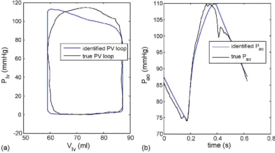
importance of the data set in Eq. (40) to accurately identify the model as well as finding a unique parameter set. The PV curve and aortic pressure waveform corresponding to the correct parameters in Fig. 8(a) are plotted in Fig. 9, showing a close match. Notice how the first third to a half of the ascending aortic pressure is matched almost exactly. The high degree of accuracy in this period is due to the parameter identification method forcing the inflection point of the model to match the inflection point of the data. This result further shows the power of the method of Fig. 3 as any feature that the model of Fig. 2(a) is capable of matching, can be precisely captured independent of starting point, with very fast convergence and very minimal computation.
It has been shown that the ascending aortic waveform inflection point is a predictive factor for all-cause and cardiovascular mortality in patients with chronic renal failure on hemodialysis [40]. Many other studies have also shown features in the continuous aortic pressure waveform to help diagnose disease states and to monitor improvements due to therapy. Therefore, this modelling and parameter identification approach has the potential to aggregate key clinical information and any significant correlations between parameters observed in the literature.
3.3.2. Parameter identification without volumes. The method of Fig. 4 with mean Vlv as an extra unknown, is
applied on two separate time periods, at 30 min and 120 min. The results of the identified parameters are compared to the parameters identified with the algorithm of Fig. 3, which are treated as the "true" parameters. For the pig at 30 min, the method identified Rmt, Rsys, Eao and Ppv with an accuracy less than 3% of the true
values, with errors of 7.6% in Ees,lvf and 18.8% in Rav. However the larger error in Rav can be attributed to the
small size of the true value for Rav. The errors for the identified left ventricle volume and pressure were 4.6% and
1.0%. For the pig at 120 min, the method identified Rmt, Rsys, Eao and Ppv with an accuracy less than 2% of the
true values, with errors of 5.1% in Ees,lvf and 14.7% in Rαu. These results combined with the simulated results in
the prior section suggest that the volume may not be needed to identify parameters, but requires further validation in clinical trials. These trials would need to use either ECG or the central pressure waveform to calculate the end-diastolic filling time. In addition, it is required to determine/define what errors in Vlv,mαx are
acceptable for diagnosis. In summary, the simulated data and the pig data with a manually chosen end-diastolic filling time from the volume profile, prove the concept that the reduced data set of Eq. (34) without mean volume is potentially sufficient for identifying parameters of the model, and warrants further investigation.
Fig. 9 - Identification results using correct parameters of Fig. 8(a). (a) Pressure-volume curve, (b) Aortic
4. Summary
Three major concepts were introduced in this paper.
• Simplified fully identifiable sub-models that closely capture a six chamber model with ventricular interaction, pericardium and inertial effects.
- The models significantly reduce computation in simulations.
- The models accurately predict both simulated response and clinically measured response.
- The major idea was to decouple the sub-models from the circulation, by changing the output parameters of the full model into unknown input parameters for the submodels. This approach ensures, that the major features of the full model are maintained, and thus in principle, is generalizable to other model structures.
• A parameter identification method based on a proportional feedback control system that iterates between a forward solution and parameter updates until the measured clinical data is precisely matched. The formulation also allows any geometrical feature that the model is capable of producing, to be precisely captured with very minimal computation, for example the end-diastolic filling time and maximum ascending aortic gradient. Once the method converges, by definition of the control system reference input, the global minimum must be reached. Therefore there can be no local minima which can commonly occur in the more traditional non-linear regression. • The reduction of the measured data set by including the removed measurements as extra unknowns in the identification method. A fast and accurate parameter identification makes this reduction possible, with minimal effect on computation. Results in both simulation and clinical data suggest the maximum and minimum volumes are not needed for an accurate identification of the model, with the addition of end-diastolic filling time and continuous ascending aortic pressure.
Current models, e.g. [41,42] are good at capturing trends in data but do not typically capture precise quantitative pressure and volume changes, including the exact measured valve timing and ascending aortic pressure profile, for individual patients. Of course in principal, complex models could be made to match to any given data set. But for limited data in an ICU setting, unique parameter identification would only be obtained if a small subset of the parameter set is optimized. Thus, the majority of parameters have to be fixed at generic values which are only ever known on a population level, not for individual patients [43-45]. Therefore, pre-determined dynamics would be assumed, which are likely wrong in fast changing critical care patients. Furthermore, a relatively large amount of computation is spent simulating these dynamics from the fixed parameters, which has no direct effect on matching a patient.
The approach in this paper is different as it only simulates the precise subset of the model that is being identified to the data. It also closely represents the corresponding sub-model of the full model and thus still maintains all the essential physiology. Therefore, very fast and unique parameter identification methods can be developed that can capture virtually any desired features with minimal effect on computational time, high accuracy and avoidance of local minima's. For example, the methods in this paper quantitatively capture the measured valve timing, where usually the qualitative trend is reported [42]. In addition, a patient specific driver function is approximately identified, without requiring the measured pressure volume curve [46].
Finally, the patient specific approach and the fast identification methods in this paper, gives the potential to analyze clinical data in an ICU of time periods of days or weeks with minimal computational time. The identified parameter changes can then be analyzed as time progresses, and trends and variations can be compared between patients. For example, population assumptions on reflex response [41,45] could be characterized within known bounds, and included in the model. Thus, the concept is to let the clinical data itself guide the modelling, with only basic model structures initially assumed in the process. The resulting model assumptions would then only be used conservatively, within the uncertainty bounds found from the retrospective studies. This approach avoids any significant pre-assumptions on patient behaviour that may hinder accurate representations of individual patient variations which are usually significant in an ICU. This paper therefore represents a set of modelling and computational tools with the potential to monitor and better manage the cardiovascular system in critical care patients.
5. Conclusions
Two simplified models of the left ventricle-systemic and right ventricle-pulmonary systems were developed that closely matched output data from a full cardiovascular system model with pericardium and ventricular interaction dynamics. The left ventricle system model was tested in simulation with up to 10% random uniformly distributed noise added to the data. The model was shown to be uniquely identifiable with the addition of the end-diastolic filling time and continuous information from the aortic pressure waveform. Furthermore, the extra data used, that is readily available in an ICU, enabled the mean volume to be added as an extra unknown parameter with minimal effect on identifiability This result has significant potential clinically, as the mean or maximum/minimum volumes are much harder to measure, where the stroke volume is relatively easy and more common.
The approach of breaking down the six chamber heart model into separate uniquely identifiable models is general in terms of decoupling parts of the circulation. This approach could in principal be applied to any complex lumped parameter CVS model. In particular, future work will utilize the simpler models to allow rapid identification of the eight chamber model [22] and any other added dynamics as required to diagnose cardiac disease states and characterize therapy response.
The clinical and simulated results both suggest that potentially better model-based diagnostic capability could be obtained with the addition of continuous aortic pressure information, and either ECG or the central venous pressure waveform to obtain the end-diastolic time. This enhanced capability has been shown to be not significantly reduced when removing volume Vlv,max/Vlv,min measurements. The results thus show the potential for
practical implementation of a model-based cardiac diagnosis/therapeutics system in the ICU based on readily measurable parameters.
REFERENCES
[1] C. Franklin, J. Mathew, Developing strategies to prevent inhospital cardiac arrest: analyzing responses of physicians and nurses in the hours before the event, Crit. Care Med. 22 (February) (1994) 244-247.
[2] G.D. Perkins, D.F. McAuley, S. Davies, F. Gao, Discrepancies between clinical and postmortem diagnoses in critically ill patients: an observational study, Crit. Care (London, England) 7 (December) (2003) R129-R132.
[3] W.R. Smith, R.M. Poses, D.K. McClish, E.C. Huber, F.L. Clemo, D. Alexander, B.P. Schmitt, Prognostic judgments and triage decisions for patients with acute congestive heart failure, Chest 121 (May) (2002) 1610-1617.
[4] D.C. Angus, W.T. Linde-Zwirble, J. Lidicker, G. Clermont, J. Carcillo, M.R. Pinsky, Epidemiology of severe sepsis in the United States: analysis of incidence, outcome, and associated costs of care, Crit. Care Med. 29 (July) (2001) 1303-1310.
[5] C. Brun-Buisson, The epidemiology of the systemic inflammatory response, Intens. Care Med. 26 (Suppl. 1) (2000) S64-S74.
[6] D.C. Angus, M.A. Kelley, R.J. Schmitz, A. White, J. Popovich Jr., Caring for the critically ill patient. Current and projected workforce requirements for care of the critically ill and patients with pulmonary disease: can we meet the requirements of an aging population? JAMA 284 (December) (2000) 2762-2770.
[7] G.W. Ewart, L. Marcus, M.M. Gaba, R.H. Bradner, J.L. Medina, E.B. Chandler, The critical care medicine crisis: a call for federal action: a white paper from the critical care professional societies, Chest 125 (April) (2004) 1518-1521.
[8] M.A. Kelley, D. Angus, D.B. Chalfin, E.D. Crandall, D. Ingbar, W. Johanson, J. Medina, C.N. Sessler, J.S. Vender, The critical care crisis in the United States: a report from the profession, Chest 125 (April) (2004) 1514-1517.
[9] R.C.P. Kerckhoffs, M.L. Neal, Q. Gu, J.B. Bassingthwaighte, J.H. Omens, A.D. McCulloch, Coupling of a 3D finite element model of cardiac ventricular mechanics to lumped systems of the systematic and pulmonic circulation, Bio med. Eng. 35 (2007) 1-18.
[10] RJ. Hunter, B.H. Smaill, Structure and function of the diastolic heart: material properties of passive myocardium, in: L. Glass, P. Hunter, A. McCulloch (Eds.), Theory of Heart, Springer-Verlag, Harrisonburg, 1991.
[11] I.J. Legrice, RJ. Hunter, B.H. Smaill, Laminar structure of the heart: mathematical model, Am. J. Physiol. 272 (1997) H2466-H2476.
[12] D.C. Chung, S.C. Niranjan, J.W. Clark Jr., A. Bidani, W.E. Johnston, J.B. Zwischenberger, D.L. Traber, A dynamic model of ventricular interaction and pericardial influence, Am. J. Physiol. 272 (1997) H2942-H2962.
[13] C. Luo, D.L. Ware, J.B.J.WC. Zwischenberger Jr., Using a human cardiopulmonary model to study and predict normal and diseased ventricular mechanics, septal interaction, and atrio-ventricular blood flow patterns, J. Cardiovasc. Eng. 7 (2007) 17-31.
[14] R. Mukkamala, R.J. Cohen, A forward model-based validation of cardiovascular system identification, Am. J. Physiol. Heart Circ. Physiol. 281 (2001) H2714-H2730.
[15] C.E. Hann, J.G. Chase, G.M. Shaw, Efficient implementation of non-linear valve law and ventricular interaction dynamics in the minimal cardiac model, Comput. Methods Prog. Biomed. 80 (October (1)) (2005) 65-74.
[16] B.W. Smith, J.G. Chase, R.I. Nokes, G.M. Shaw, G. Wake, Minimal haemodynamic system model including ventricular interaction and valve dynamics, Med. Eng. Phys. 26 (2) (2004) 131-139.
[17] G. Pillonetto, G. Sparacino, C. Cobelli, Numerical non-identifiability regions of the minimal model of glucose kinetics: superiority of Bayesian estimation, Math. Biosci. 184 (2003) 53-67.
[18] K. Thomaseth, C. Cobelli, Generalized sensitivity functions in physiological system identification, Ann. Biomed. Eng. 27 (1999) 607-616.
[19] S. Audoly, L. DAngio, M.P. Saccomani, C. Cobelli, Global identifiability of linear compartmental models—a computer algebra algorithm, IEEE Trans. Biomed. Eng. 45 (January) (1998) 36-47.
[20] S. Audoly, G Bellu, L. DAngio, M.P. Saccomani, C. Cobelli, Global identifiability of nonlinear models of biological systems, IEEE Trans. Biomed. Eng. 48 (January) (2001) 55-65.
[21] C. Starfinger, C.E. Hann, J.G. Chase, T. Desaive, A. Ghuysen, G.M. Shaw, Model-based cardiac diagnosis of pulmonary embolism, Comput. Methods Prog. Biomed. 87 (July (1)) (2007) 46-60.
[22] C. Starfinger, J.G. Chase, C.E. Hann, G.M. Shaw, B. Lambermont, A. Ghuysen, P. Kolh, P. Dauby, T. Desaive, Model-based identification and diagnosis of a porcine mode of induced endotoxic shock with hemofiltration, Math. Biosci. 216 (2) (2008) 132-139.
[23] C. Starfinger, J.G. Chase, C.E. Hann, G.M. Shaw, P. Lambert, B.W. Smith, E. Sloth, A. Larsson, S. Andreassen, S. Rees, Model-based identification of PEEP titrations during different volemic levels, Comput. Methods Prog. Biomed. 91 (2) (2008) 135-144.
[24] C. Starfinger, J.G. Chase, C.E. Hann, G.M. Shaw, P. Lambert, B.W. Smith, E. Sloth, A. Larsson, S. Andreassen, S. Rees, Prediction of hemodynamic changes towards PEEP titrations at different volemic levels using a minimal cardiovascular model, Comput. Methods Prog. Biomed. 91 (2) (2008) 128-134
[25] A.C. Guyton, J.E. Hall, Textbook of Medical Physiology, 10th ed., W.B. Saunders Company, Philadelphia, 2000.
[26] C.E. Hann, J.G. Chase, G.M. Shaw, Integral-based identification of patient specific parameters for a minimal cardiac model, Comput. Methods Prog. Biomed. 81 (February (2)) (2006) 181-192.
[27] R. Shabetai, The Pericardium, Kluwer Academic Publishers, 2003.
[28] J. Sutton, D.C. Gibson, Measurement of postoperative pericardial pressure in man, Br. Heart J. 39 (1977) 1-6.
[29] W.P. Santamore, D. Burkhoff, Hemodynamic consequences of ventricular interaction as assessed by model analysis, Am. J. Physiol. 260 (1991) H146-H157.
[30] B.W. Smith, S. Andreassen, G.M. Shaw, PL. Jensen, S.E. Rees, J.G. Chase, Simulation of cardiovascular system diseases by including the autonomic nervous system in a minimal model, Comput. Methods Prog. Biomed. 86 (2) (2007) 153-160.
[31] B.W. Smith, J.G. Chase, G.M. Shaw, R.I. Nokes, Experimentally verified minimal cardiovascular system model for rapid diagnostic assistance, Control Eng. Pract. 13 (September) (2005) 1183-1193.
[32] C. Hann, J. Chase, S. Andreassen, B. Smith, G. Shaw, Diagnosis using a minimal cardiac model including reflex actions, Intens. Care Med. 31 (2005) S18.
[33] C. Hann, S. Andreassen, B. Smith, G. Shaw, J. Chase, Identification of time-varying cardiac disease state using a minimal cardiac model with reflex actions, in: Proceedings of the 14th IFAC Symposium on System Identification (SYSID 2006), Newcastle, Australia, 2006, pp. 475-480.
[34] I.K. Youssef, H.A. El-Arabawy, Picard iteration algorithm combined with Gauss-Seidel technique for initial value problems, Appl. Math. Comput. 190 (1) (2007) 345-355.
[35] G.P. Rao, H. Unbehauen, Identification of continuous-time systems, IEE Proc. Control Theory Appl. 153 (2) (2006) 185-220.
[36] E.R. Carson, C. Cobelli, Modelling Methodology for Physiology and Medicine, Academic Press, San Diego, 2001.
[38] A. Ghuysen, B. Lambermont, P. Kolh, V. Tchana-Sato, D. Magis, P. Gerard, M. Mommens, N. Janssen, T. Desaive, V. D'Orio, Alteration of right ventricular-pulmonary vascular coupling in a porcine model of progressive pressure overloading, Shock 29 (2) (2007) 197-204.
[39] A. Ghuysen, B. Lambermont, P. Kolh, V. Tchana-Sato, D. Magis, P. Gerard, M. Mommens, N. Janssen, T. Desaive, V. D'Orio, Alteration of right ventricular-pulmonary vascular coupling in a porcine model of progressive pressure overloading, Shock 29 (2007) 197-204.
[40] H. Ueda, T. Hayashi, K. Tsumura, K. Yoshimaru, Y. Nakayama, J. Yoshikawa, Inflection point of ascending aortic waveform is a predictive factor for all-cause and cardiovascular mortality in patients with chronic renal failure on hemodialysis, Am. J. Hypertens. 17 (2004) 1151-1155.
[41] R. Mukkamala, R.J. Cohen, A forward model-based validation of cardiovascular system identification, Am. J. Physiol. Heart Circ. Physiol. 281 (6) (2001) H2714-2730.
[42] R.C. Kerckhoffs, M.L. Neal, Q, Gu, J.B. Bassingthwaighte, J.H. Omens, A.D. McCulloch, Coupling of a 3D finite element model of cardiac ventricular mechanics to lumped systems models of the systemic and pulmonic circulation, Ann. Biomed. Eng. 35 (2006) 1-18.
[43] F. Liang, H. Liu, A closed-loop lumped parameter computational model for human cardiovascular system, JSME Int. J. Ser. C 48 (2005) 484-493.
[44] R. Mukkamala, K. Toska, R.J. Cohen, Noninvasive identification of the total peripheral resistance baroreflex, Am. J. Physiol. Heart Circ. Physiol. 284 (3) (2003) 947-959.
[45] E.B. Shim, J.Y. Sah, C.H. Youn, Mathematical modeling of cardiovascular system dynamics using a lumped parameter method, Jpn. J. Physiol. 54 (6) (2004) 545-553.
[46] H. Senzaki, C.H. Chen, D.A. Kass, Single-beat estimation of end-systolic pressure-volume relation in humans a new method with the potential for noninvasive application, Circulation 94 (10) (1996) 2497-2506.