News Arrival, Jump Dynamics and Volatility Components for Individual Stock Returns

Texte intégral

(1)2003s-38. News Arrival, Jump Dynamics and Volatility Components for Individual Stock Returns John M. Maheu, Thomas H. McCurdy. Série Scientifique Scientific Series. Montréal Juin 2003. © 2003 John M. Maheu, Thomas H. McCurdy. Tous droits réservés. All rights reserved. Reproduction partielle permise avec citation du document source, incluant la notice ©. Short sections may be quoted without explicit permission, if full credit, including © notice, is given to the source..

(2) CIRANO Le CIRANO est un organisme sans but lucratif constitué en vertu de la Loi des compagnies du Québec. Le financement de son infrastructure et de ses activités de recherche provient des cotisations de ses organisationsmembres, d’une subvention d’infrastructure du ministère de la Recherche, de la Science et de la Technologie, de même que des subventions et mandats obtenus par ses équipes de recherche. CIRANO is a private non-profit organization incorporated under the Québec Companies Act. Its infrastructure and research activities are funded through fees paid by member organizations, an infrastructure grant from the Ministère de la Recherche, de la Science et de la Technologie, and grants and research mandates obtained by its research teams. Les organisations-partenaires / The Partner Organizations PARTENAIRE MAJEUR . Ministère du développement économique et régional [MDER] PARTENAIRES . Alcan inc. . Axa Canada . Banque du Canada . Banque Laurentienne du Canada . Banque Nationale du Canada . Banque Royale du Canada . Bell Canada . Bombardier . Bourse de Montréal . Développement des ressources humaines Canada [DRHC] . Fédération des caisses Desjardins du Québec . Gaz Métropolitain . Hydro-Québec . Industrie Canada . Ministère des Finances [MF] . Pratt & Whitney Canada Inc. . Raymond Chabot Grant Thornton . Ville de Montréal . École Polytechnique de Montréal . HEC Montréal . Université Concordia . Université de Montréal . Université du Québec à Montréal . Université Laval . Université McGill ASSOCIÉ AU : . Institut de Finance Mathématique de Montréal (IFM2) . Laboratoires universitaires Bell Canada . Réseau de calcul et de modélisation mathématique [RCM2] . Réseau de centres d’excellence MITACS (Les mathématiques des technologies de l’information et des systèmes complexes) Les cahiers de la série scientifique (CS) visent à rendre accessibles des résultats de recherche effectuée au CIRANO afin de susciter échanges et commentaires. Ces cahiers sont écrits dans le style des publications scientifiques. Les idées et les opinions émises sont sous l’unique responsabilité des auteurs et ne représentent pas nécessairement les positions du CIRANO ou de ses partenaires. This paper presents research carried out at CIRANO and aims at encouraging discussion and comment. The observations and viewpoints expressed are the sole responsibility of the authors. They do not necessarily represent positions of CIRANO or its partners.. ISSN 1198-8177.

(3) News Arrival, Jump Dynamics and Volatility Components for Individual Stock Returns* John M. Maheu†, Thomas H. McCurdy‡. Résumé / Abstract Cet article modélise les différentes composantes de la distribution des rendements qui sont supposés être régis par un processus latent de nouvelles. La variance conditionnelle des rendements est une combinaison de sauts et de composantes qui varient continûment. Ce mélange permet de capter les grands changements occasionnels de prix qui sont dus à l'impact des nouvelles, telles que des surprises dans les revenus d'une compagnie, aussi bien que des changements plus lisses des prix qui peuvent résulter de transactions de liquidité ou de transactions stratégiques au fur et à mesure que l'information est disséminée. À la différence des modèles classique de sauts SV, les réalisations précédentes des sauts et des innovations normales peuvent intervenir asymétriquement dans la volatilité espérée. Il s'agit d'une nouvelle source d'asymétrie qui améliore les prévisions de volatilité, en particulier après de grands mouvements tels que le crash de 87. Un processus de Poisson hétérogène régit la probabilité des sauts et est représenté par un paramètre d'intensité conditionnelle qui varie dans le temps. Le modèle est appliqué aux rendements de différentes compagnies et à trois indices. Nous montrons ainsi empiriquement l'impact et les effets de rétroaction des sauts par rapport aux innovations normales, les effets de leviers simultanés et décalés, la dynamique de série temporelle du groupement des sauts, et l'importance de modéliser la dynamique des sauts dans les périodes de volatilité élevée. Mots clés : composantes de volatilité, impact des nouvelles, intensité conditionnelle des sauts, taille des sauts, effets de levier, filtre.. *. We are grateful to the editor and an anonymous referee for very helpful comments. We also thank participants at the Modeling, Estimating and Forecasting Volatility Conference (University of Montreal), the Financial Mathematics Seminar (Fields Institute), the North American Summer Meeting of the Econometric Society (Los Angeles), the Northern Finance Association 2002 Meetings, the Canadian Econometrics Study Group, the Waterloo Financial Econometrics Conference, workshops at Queen’s University, and University of Toronto, as well as, Toby Daglish, J.C. Duan, Adlai Fisher and Nour Meddahi for helpful comments. Both authors also thank the Social Sciences and Humanities Research Council of Canada for financial support. † Department of Economics, University of Toronto, jmaheu@chass.utoronto.ca. ‡ Joseph L. Rotman School of Management, University of Toronto, and CIRANO, tmccurdy@rotman.utoronto.ca..

(4) This paper models different components of the return distribution which are assumed to be directed by a latent news process. The conditional variance of returns is a combination of jumps and smoothly changing components. This mixture captures occasional large changes in price, due to the impact of news innovations such as earnings surprises, as well as smoother changes in prices which can result from liquidity trading or strategic trading as information disseminates. Unlike typical SV-jump models, previous realizations of both jump and normal innovations can feedback asymmetrically into expected volatility. This is a new source of asymmetry (in addition to good versus bad news) that improves forecasts of volatility particularly after large moves such as the ’87 crash. A heterogeneous Poisson process governs the likelihood of jumps and is summarized by a time varying conditional intensity parameter. The model is applied to returns from individual companies and three indices. We provide empirical evidence of the impact and feedback effects of jump versus normal return innovations, contemporaneous and lagged leverage effects, the time-series dynamics of jump clustering, and the importance of modeling the dynamics of jumps around high volatility episodes. Keywords: volatility components, news impacts, conditional jump intensity, jump size, leverage effects, filter..

(5) I. Introduction There is a wide-spread perception in the financial press that volatility of asset returns has been changing. The new economy is introducing more uncertainty. Indeed, it can be argued that volatility is being transferred from the economy at large into the financial markets, which bear the necessary adjustment shocks.1 Given the impact of changes in volatility dynamics on many important financial and economic decisions (such as, portfolio re-balancing, derivative pricing, risk measurement and management), it is important to assess the empirical validity of this perception and to investigate the sources and characteristics of changing volatility dynamics. Volatility2 and risk can be linked to the quantity and quality of information pertaining to a stock’s expected future earnings and cash flows. For example, information that results in a resolution of uncertainty about a firm’s future prospects can result in a large revision in current prices. According to this view, the most important process affecting price movements is the news arrival process. In Ross (1989) and Andersen (1996) the volatility of stock price changes is directly related to the rate of flow of information to the market. For individual securities, news about anticipated cash flows and the appropriate discount rate are particularly relevant. A noteworthy contribution in this vein is a recent study by Campbell, Lettau, Malkiel, and Xu (2001) who report that firm-level variance has more than doubled between 1962 and 1997 whereas market and industry variances have remained fairly stable over that period.3 They analyze the dynamics of idiosyncratic, industry and market components of the volatility of individual stock returns. We study the distributional components, in particular, large versus small changes of stock returns; and how these components contribute to the dynamics of volatility and higher-order moments of returns. In this paper we do not model the latent news process directly but rather propose a model of the conditional variance of returns implied by the impact of different types of news. We interpret the innovation to returns, which is directly measurable from price data, as the news impact from latent news innovations. The latent news process is postulated to have two separate components, normal news and unusual news events, which have different impacts on returns and expected volatility for individual stocks.4 Normal news innovations are assumed to cause smoothly evolving changes in the conditional 1. ”Coping with the market’s mood swings”, Financial Times, London, Sept. 27, 2000. In this paper we use the term volatility to refer generically to information on the second moment of returns. 3 Although systematic market risk is an important part of many financial decisions, Campbell, Lettau, Malkiel, and Xu (2001) emphasize that the total volatility of a firm’s return is also relevant (for arbitrageurs, for derivative pricing, for hedge funds, etc.). 4 Clark (1973) and Tauchen and Pitts (1983) use information flows to motivate price movements and trading activity. Andersen (1996) concludes that ”it is natural to hypothesize that there are two 2. 1.

(6) variance of returns. The second component of the latent news process causes infrequent large moves in returns. The impacts of these unusual news events are labelled jumps. Therefore, the news process induces two components in returns which are identified by their volatility dynamics and higher order moments. We model these components as normal innovations, and abnormal or jump innovations. A potential source of jump innovations to returns can be important news events, such as earnings surprises. For example, in January 2000, Intel Corporation announced earnings that were 8.83% higher than the mean IBES forecast. This earnings surprise resulted in a 12.4% increase in price on January 14, 2000. In October 2000 IBM’s negative earnings surprise of -0.18% led to a price change of -16.9% on October 18, 2000. On November 13th, 2000, an earnings surprise of -19.76% for Hewlett-Packard resulted in a price change of -13.67%. These news surprises concerning expected future cash flows resulted in price changes well above normal and might be better captured by jumps rather than Brownian motion or normal innovations. On the other hand, less extreme movements in price (modeled as normal innovations) can be due to typical news events as well as liquidity trading and strategic trading as information disseminates.5 To augment Brownian motion in an attempt to better capture the empirical distribution of returns, Press (1967) introduced a jump-diffusion model which assumes information arrivals are independently and identically distributed as a Poisson process. Over an interval (t-1,t) a random number of news events arrive. In this compound events model, the Poisson distribution directs the number of jump events occurring in the fixed interval. The expected number of events per interval is defined as the intensity (jump frequency) of the Poisson process. Associated with each of these news events is a jump size which is assumed to be stochastic. This basic jump-diffusion model and its many extensions can be applied to the effect of news flows on price changes. Of particular relevance to our application are those that also incorporate autoregressive stochastic volatility (SV). Traditional SV-jump-diffusion specifications assume a temporally independent arrival rate of jump events. There is evidence that, like the information process itself, jumps tend to be clustered together. Not only do we observe sustained episodes of extreme volatility (for example, the SE Asian currency crisis), but even market crashes can be realized in a series of jumps over a short period of time. Allowing for time variation and clustering in the process governing jumps may be important. For example, Bates (1991) finds systematic behavior in the expected number of jumps around the 1987 crash using options data. Recent examples of SV-jump-diffusion specifications with time-varying jump intensities include Andersen, Benzoni, and Lund (2002), Bates (2000), Chernov, or more types of information arrival processes that have different implications for volume and return volatility persistence”. 5 Glosten and Milgrom (1985) and Andersen (1996) develop a market microstructure model in which asymmetric information and liquidity requirements induce trades in response to information arrivals. They outline how a news event that causes a large price change can be associated with quite different volatility effects than one with less information content. Bates (2001) provides a theoretical model in which investor heterogeneity affects the impact of news events on asset prices.. 2.

(7) Gallant, Ghysels, and Tauchen (2003), and Pan (2002).6 Eraker, Johannes, and Polson (2003) allow for jumps in both returns and volatility. We explore dependence in the arrival process governing jump events in a discretetime setting and extend the work of Jorion (1988) and Vlaar and Palm (1993), among others.7 Bates and Craine (1999) allow a volatility factor to drive the intensity. Bekaert and Gray (1998), Das (2002), and Neely (1999) allow financial and macroeconomic variables to affect the jump intensity. Johannes, Kumar, and Polson (1999) consider a state dependent jump model which allows past jumps and observables to affect the jump probability. We develop a mixed GARCH-jump model incorporating the autoregressive conditional jump intensity parameterization proposed by Chan and Maheu (2002). Maintaining distributional assumptions at the relevant discrete-time frequency allows us to use maximum likelihood estimation and the associated filter to infer the distribution of the unobservable jumps. The conditional intensity process allows the expected arrival rate of jumps to vary over time and allows jumps to cluster. The time variation in the conditional intensity implies all high order conditional moments of returns are time varying. Similar to a Peso problem, jumps need not occur to have important effects on the conditional higher-order moments. Linked to a particular jump event is the news impact that the jump has on price changes. Depending on the type and the importance of the information revealed by the news, the stochastic jump size may be negative, positive, big or small. For example, jumps can reflect good or bad news events and affect the conditional and unconditional skewness of the return distribution through the magnitude and the sign of the mean of the jump size distribution. Therefore, the dynamics of volatility are affected by a time-varying rate of jump arrival, stochastic jump size, and volatility clustering. The conditional variance in our model is a combination of a smoothly evolving continuous-state GARCH component and a discrete jump component. In addition, unlike conventional parameterizations of SV-jump-diffusions, previous realizations of both normal and jump innovations affect expected volatility through the GARCH component of the conditional variance.8 This feedback can be important because once return innovations are realized, there may be strategic trading related to the propagation of the news, liquidity trading, etc. These activities are further sources of volatility clustering – in addition to clustering of jump arrivals. We allow for several asymmetric responses to past return innovations. Firstly, the news impact resulting in jump innovations can have a different feedback on expected 6. Yu (1999) has proposed a pure jump diffusion with a time-varying intensity. For example, Baillie and Han (2001), Pan (1997), Nieuwland, Vershchoor, and Wolff (1994), Feinstone (1987), and Ball and Torous (1983). Oomen (2002) discusses various extensions including a multiple component compound Poisson model for high and low frequency jumps. 8 GARCH specifications allow past (squared) return innovations to feedback into expected volatility. Engle and Ng (1993) interpret the return innovation as the impact of news events. Their news impact curve summarizes the possibly asymmetric impact of good and bad news on the conditional variance of next period’s return. 7. 3.

(8) volatility than the news impact associated with normal innovations. For instance, important news innovations that result in a jump may be quickly incorporated into current prices and have a smaller effect on expected volatility; or the reverse, news that results in jumps may cause future volatility. Secondly, we allow for asymmetric responses to good versus bad news in the GARCH component of volatility.9 A further flexibility is that the asymmetric effect of good vs bad news can be different for jump versus normal innovations. These novel features allow a richer characterization of volatility dynamics, particularly with respect to events in the tail of the distribution. We initially apply our model to equity returns from eleven U.S. stocks. To show that jumps may be associated with significant news innovations, we have computed the probability of jumps (inferred from our model) around days that earnings surprises were announced. We find empirical support for our conjecture that large innovations to returns are associated with significant news events. For the examples discussed above, the ex post probability of a jump for Intel is .94 (January 14, 2000), IBM .99 (October 18, 2000) and Hewlett-Packard .74 (November 13, 2000). Consistent with previous studies we find that the unconditional jump intensity is low. However, since the conditional jump intensity is autoregressive, jumps are likely to cluster. Therefore, IBM may have 3 jumps within a week but no jumps for the next 3 months. On average, jumps account for about 25% of daily volatility. Yet, when jumps occur, their proportion of the conditional variance can shoot up to 90%. Statistical tests strongly reject a constant intensity version of the model in favor of autocorrelation in the jump intensity. This time variation is very important in capturing return dynamics. For example, by correctly predicting the jumps following the 1987 crash, the model’s predictions of IBM daily volatility closely match the quick return of realized volatility to normal levels. In contrast, we show that a benchmark asymmetric GARCH model with t-distributed innovations but no jumps takes a significant period of time to return to normal levels of volatility. Jumps affect forecasts of future volatility directly through the time-varying Poisson arrival process. In addition, the effect of jumps on the conditional variance through GARCH feedback effects is also statistically significant. However, jump innovations tend to have a smaller feedback coefficient than normal innovations. This evidence is consistent with the stylized fact10 that the persistence effect on expected volatility from large shocks to returns is often smaller than normal innovations. Although we find the traditional good and bad news asymmetry associated with the GARCH volatility component, this appears to operate mostly when no jumps occur. In contrast, in the presence of jumps the news impact curve displays less asymmetry. 9. Asymmetric GARCH models include Engle and Ng (1993), Glosten, Jagannathan, and Runkle (1993) and the Nelson (1991) EGARCH specification. The empirical stylized fact that negative return (bad news) innovations are associated with increases in volatility has become known as the leverage effect. Cho and Engle (1999) and Campbell and Hentschel (1992) provide an economic interpretation of news effects through asymmetric volatility and its effect on the required rate of return from stocks. 10 For example, Schwert (1990) and Engle and Mustafa (1992).. 4.

(9) It is interesting to note that the effects of jumps appear to be different for new versus traditional economy stocks. To investigate further, we apply our model to three indices of different types of firms: the DJIA, the NASDAQ 100, and the CBOE Technology index (TXX). The more volatile indices have more frequent jumps and these jumps have a larger impact on the return distribution. All indices display significant jump clustering. This result is consistent with evidence reported in Johannes, Kumar, and Polson (1999). The jump size mean is significantly negative for all three indices. This implies a negative conditional correlation between jump innovations and squared return innovations. In other words, large negative return realizations are associated with an immediate increase in the variance. We call this a contemporaneous leverage effect. Note that this leverage effect is time varying due to the time-varying correlation. This result of a significant contemporaneous asymmetry is associated with a somewhat weaker asymmetry between the sign of lagged innovations and the GARCH variance component. For our samples of indices, a contemporaneous leverage effect which is captured directly by jumps is more important than the lagged leverage effect which is captured by the GARCH feedback structure. These results extend the evidence obtained from traditional GARCH models. The structure of our model is such that the mixture of components can adapt flexibly to capture different features of the conditional distribution of returns. However, introducing more parameters involves the danger of over fitting in sample. Therefore, it is important to determine whether or not the improved in-sample fit is useful for forecasting out of sample. Using a range-based measure for ex post or realized volatility, we demonstrate that for ten of eleven firms our model has superior out-of-sample forecasts relative to a benchmark asymmetric GARCH model with fat-tailed innovations. In addition, we provide evidence of superior out-of-sample forecasts for high volatility periods and for conditional forecasts following large negative moves in the market. The latter two tests are designed to evaluate the dynamics in the tails of the return distribution. In summary, our paper provides evidence of time dependence in jump intensities for both individual stocks and indices using an autoregressive conditional jump intensity parameterization; allows both normal and jump innovations to feedback into expected volatility; and provides new results on asymmetric effects of return innovations on volatility. Conditional skewness and kurtosis are functions of both volatility components. The conditional skewness result can be interpreted as a time-varying contemporaneous leverage effect. This is modeled jointly with the possibility of lagged leverage effects through the GARCH feedback structure. These novel features allow the model to perform better around crash periods and other events in the tail of the distribution. With regard to the indices studied in this paper, we document several differences between volatility components associated with ’old’ versus ’new economy’ stocks. Finally, our model provides superior out-of-sample conditional variance forecasts relative to a popular benchmark model, even when the latter is allowed to have fat-tailed innovations. These superior out-of-sample forecasts should result in improvements in financial management.. 5.

(10) This paper is organized as follows. Section II gives a detailed account of the two stochastic components affecting returns, construction of the likelihood, and conditional moments. The data used in this study is presented in Section III. A discussion of the empirical results is presented in Section IV, out-of-sample forecasts are evaluated in Section V, while Section VI summarizes the results. An appendix contains some theoretical calculations for the model.. II. A GARCH-Jump Model for Returns In this section we present a mixed GARCH-jump model for individual security returns. In our model of return volatility, we maintain an unobserved news process that directs movements in prices. News events, together with investors’ expectations of these events, may result in price changes. In this paper we do not model the latent news process directly but rather propose a model of the conditional variance of returns implied by the impact of different types of news. We label the innovation to returns, which is directly measurable from price data, as the news impact from latent news innovations. The latent news process is postulated to have two separate components, normal and unusual news events. These news innovations are identified through their impact on return volatility. In particular, the impact of unobservable normal news innovations is assumed to be captured by the return innovation component, ²1,t . This component of the news process causes smoothly evolving changes in the conditional variance of returns. The second component of the latent news process causes infrequent large moves in returns, ²2,t . The impact of these unusual news events are labelled jumps. We begin by specifying the components of returns. Given an information set at time t − 1, which consists of the history of returns Φt−1 = {rt−1 , ..., r1 }, the two stochastic innovations, ²1,t and ²2,t , drive returns, rt = µ + ²1,t + ²2,t .. (1). ²1,t is a mean-zero innovation (E[²1,t |Φt−1 ] = 0) with a Normal stochastic forcing process, ²1,t = σt zt , zt ∼ N ID(0, 1),. (2). ²2,t is a jump innovation specified so that it is also conditionally mean zero (E[²2,t |Φt−1 ] = 0), and ²1,t is contemporaneously independent of ²2,t . The subsections that follow describe our parameterization of these two stochastic components of returns. In particular, we begin by specifying the process governing jumps and the distribution of jump sizes. Then we describe in some detail the components of time-varying volatility. These parametric assumptions allow us to optimally infer when jumps arrive through the use of Bayes rule. The next subsections summarize the conditional moments of returns and the construction of the loglikelihood and the filter. Henceforth, we refer to the mixed GARCH-jump model with autoregressive jump intensity as GARJI. 6.

(11) A. Autoregressive conditional jump intensity (ARJI) Unlike the previously cited GARCH-jump mixture models, we explicitly incorporate an autoregressive conditional intensity that governs the likelihood of jumps occurring between time t − 1 and t. The distribution of jumps is assumed to be Poisson with a time-varying conditional intensity parameter. In particular, a Poisson distribution with parameter λt conditional on Φt−1 is assumed to describe the arrival of a discrete-valued number of jumps, nt ∈ {0, 1, 2, ...}, over the interval (t − 1, t). The conditional density of nt is, exp(−λt )λjt P (nt = j|Φt−1 ) = j = 0, 1, 2, . . . (3) j! The conditional jump intensity, λt ≡ E[nt |Φt−1 ], is the expected number of jumps conditional on the information set Φt−1 . The dynamics governing λt are parameterized as λt = λ0 + ρλt−1 + γξt−1 , (4) defined as an autoregressive conditional jump intensity (ARJI) model in Chan and Maheu (2002). In this model the conditional jump intensity λt is assumed to be autoregressive and related to last period’s conditional intensity as well as to an intensity residual ξt−1 . It seems likely that the probability of jumps will vary over time, and may be sensitive to economic conditions, such as the business cycle, bull and bear markets and monetary policy. The specification in Equation 4 is a time-series approach to studying the arrival process of jumps.11 A natural measure of the persistence of this process is ρ. The restrictions ρ = γ = 0 yield a constant jump intensity as in Jorion (1988). The jump intensity residual is defined as, ξt−1 ≡ E[nt−1 |Φt−1 ] − λt−1 ∞ X = jP (nt−1 = j|Φt−1 ) − λt−1 .. (5). j=0. P (nt−1 = j|Φt−1 ) is called the filter and is the ex post inference on nt−1 given time t − 1 information. More details on the filter and construction of the loglikelihood are detailed in a subsection below. E[nt−1 |Φt−1 ] is our ex post assessment of the expected number of jumps that occurred from t − 2 to t − 1, while λt−1 is by definition the conditional expectation of nt−1 given the information set Φt−2 . Therefore, ξt−1 represents the change in the econometrician’s conditional forecast of nt−1 as the information set is updated (ξt−1 = E[nt−1 |Φt−1 ] − E[nt−1 |Φt−2 ]). Note from this definition that ξt is a martingale difference sequence with respect to Φt−1 , E[ξt |Φt−1 ] = 0 11. (6). An alternative model of the conditional intensity would be a structural model in which economic variables affect the jump likelihood.. 7.

(12) and therefore E[ξt ] = 0 and Cov(ξt , ξt−i ) = 0, i > 0. Hence, the intensity residuals in a well specified model should display no autocorrelation. There are several important features of this conditional intensity model. First, if the ARJI specification is stationary, (|ρ| < 1), then the unconditional jump intensity is equal to λ0 E[λt ] = . (7) 1−ρ Second, forecasts of λt+i , and therefore the conditional variance of ²2,t+i , are straightforward to calculate. For example, multiperiod forecasts of the expected number of future jumps are ½ λt i=0 E[λt+i |Φt−1 ] = (8) i−1 i λ0 (1 + ρ + · · · + ρ ) + ρ λt i ≥ 1 Notice that the ARJI model can be re-expressed as, λt = λ0 + (ρ − γ)λt−1 + γE[nt−1 |Φt−1 ].. (9). Therefore, subject to reasonable startup conditions that ensure λ1 > 0, a sufficient condition for λt > 0 for all t is λ0 > 0, ρ ≥ γ, and γ ≥ 0.12 To estimate the ARJI model, startup values of λt , ξt , t = 0 must be set. We set startup values of the jump intensity to the unconditional value in Equation 7, and ξ0 = 0.. B. The jump innovation and jump-size distribution The jump size Yt,k is assumed to be independently drawn from a Normal distribution. The jump-size distribution is Yt,k ∼ N ID(θ, δ 2 ), (10) and the jump component affecting returns from t − 1 to t (period t) is Jt =. nt X. Yt,k .. (11). k=1. Therefore, the jump innovation associated with period t is expressed as ²2,t = Jt − E[Jt |Φt−1 ] =. nt X. Yt,k − θλt ,. (12). k=1. which is the sum of the stochastic nt jumps which arrived over the time interval (t − 1, t) adjusted by E[Jt |Φt−1 ] = θλt , so that ²2,t is conditionally mean zero. 12. Note that if ρ < γ, additional restrictions on the model may be available to ensure λt > 0 for all t.. 8.

(13) C. Time-varying volatility components The conditional variance of returns is decomposed into two separate components: a smoothly evolving conditional variance component related to the diffusion of past news impacts; and the conditional variance component associated with the heterogeneous information arrival process which generates jumps. The conditional variance of returns is, Var(rt |Φt−1 ) = Var(²1,t |Φt−1 ) + Var(²2,t |Φt−1 ). (13) The first component of the conditional variance, σt2 ≡ Var(²1,t |Φt−1 ), is parameterized as a GARCH function of past return innovations, 2 σt2 = ω + g(Λ, Φt−1 )²2t−1 + βσt−1 ,. (14). where g(·) is a function of the parameter vector Λ, and the information set and ²t−1 = ²1,t−1 + ²2,t−1 ,. (15). is the total return innovation observable at time t − 1. We label g(·) the feedback coefficient from past return innovations. The GARCH volatility component allows past shocks affecting returns to affect expected volatility, and captures the smooth autoregressive changes in the conditional variance that are predictable based on past news impacts. Following Engle and Ng (1993), we associate good news with a positive impact on returns, (²t−1 > 0) and bad news with a negative impact on returns, (²t−1 < 0). The g(·) function detailed below allows for asymmetric effects with respect to the impact of past good and bad news and also with respect to feedback effects from past jump versus normal innovations. Ideally we want each component of ²t−1 to affect future expected volatility differently.13 However, we cannot perfectly separate these two stochastic components based on observed returns.14 Instead, our GARCH specification allows the feedback from ²t−1 to flexibly respond to the composition of ²t−1 through the parameter function g(Λ, Φt−1 ). Volatility may be sensitive to good news vs bad news effects or whether a jump occurred last period. For instance, important news events that result in a jump may be quickly incorporated into current prices and have a smaller effect on future volatility; or the reverse, news that causes jumps may cause future volatility.15 To investigate this hypothesis we estimate the number of jumps that occurred during period t-1 and allow it 13. Note that measurable shocks to the conditional intensity do propagate and affect future jump probability (and therefore expected volatility) separately from the GARCH specification. 14 We can calculate E[²2,t−1 |Φt−1 ], but this is likely to seriously understate the variability from the realized ²2,t−1 . 15 Important news events may cause future volatility as investors absorb the importance of the news and its effect on future cash flows and the profitability of the firm. Often important news events stay in the headlines for several days forcing investors to reevaluate their expectations.. 9.

(14) to directly affect the feedback that ²t−1 has on the GARCH variance process. We allow for all of these responses using the following parameterization:16 g(Λ, Φt−1 ) = exp(α + αj E[nt−1 |Φt−1 ] + I(²t−1 )(αa + αa,j E[nt−1 |Φt−1 ])),. (16). where the model parameters are collected in the vector Λ = {α, αj , αa , αa,j }, I(²t−1 ) is an indicator function which takes the value 1 when ²t−1 < 0 and 0 otherwise, and E[nt−1 |Φt−1 ] is an ex post assessment of the expected number of jumps that occurred between t − 2 and t − 1, using t − 1 information. Firstly, this parameterization of σt2 allows asymmetric responses to bad versus good news. In particular, observed negative innovations to returns (bad news) are allowed to have a different feedback on σt2 through the extra contribution of the parameters αa and αa,j . Recall that the GARCH parameterization includes the effects of both past normal innovations and past jump innovations to returns, as indicated by (15). Our parameterization allows for a difference in the propagation of previous news effects which result in jumps (²2,t−1 ) versus news events that cause normal innovations (²1,t−1 ). Therefore, the parameter αj , scaled by the most recently inferred number of jumps, allows the feedback on σt2 from news events causing jumps to be different than the feedback associated with normal news events. In addition, we allow the news feedback on σt2 from the inferred number of jumps to be different when the past news was good or bad. To illustrate: if last period’s news was good and no jumps occurred, the feedback coefficient to σt2 is g(Λ, Φt−1 ) = exp(α) while if news was good and one jump occurred, the coefficient is g(·) = exp(α + αj ); if last periods news was bad and no jump occurred, the feedback coefficient to σt2 is g(·) = exp(α+αa ); and finally, if the news was bad and was associated with one jump it is g(·) = exp(α + αa + αj + αa,j ). Given our development of the conditional jump intensity and the jump-size distribution, the conditional variance component associated with the jump innovation is, Var(²2,t |Φt−1 ) = (θ2 + δ 2 )λt .. (17). This contribution to the conditional variance from jumps will vary over time as the conditional intensity λt varies. In other words, this component can range from being small to large as the expected number of jumps changes through time. One interpretation of the decomposition of the conditional variance into the two components is that the GARCH component σt2 captures the normal time-variation of volatility associated with the predictable decay of the impact, on expected volatility, from past news innovations to returns. We interpret this time-series effect to be related to the dissemination and diffusion of information, liquidity trading, etc. In contrast to the GARCH specification of volatility, jumps occur when a significant news event arrives which causes an unusual abrupt change in returns. For instance, a jump is 16. Along with non-negative constraints on ω and β, the exponential function ensures that the conditional variance is positive.. 10.

(15) likely to have occurred when an extreme tail realization occurs in the returns process. Statistically, jumps are identified by observations that are inconsistent with the first stochastic component of returns, ²1,t . In this case, the GARCH volatility component is unable to accommodate the abrupt change in volatility and such observations are identified as a jump. Modeling jumps and their arrival process may be a particularly important feature for capturing events which lead to episodes of high volatility as well as for incorporating higher-order conditional moment dynamics, such as time-varying skewness and kurtosis of stock returns.. D. Moments of returns The first four conditional moments of returns for our model are, E[rt |Φt−1 ] = µ Var(rt |Φt−1 ) = σt2 + (θ2 + δ 2 )λt λt (θ3 + 3θδ 2 ) Sk(rt |Φt−1 ) = (σt2 + λt δ 2 + λt θ2 )3/2 λt (θ4 + 6θ2 δ 2 + 3δ 4 ) . Ku(rt |Φt−1 ) = 3 + (σt2 + λt δ 2 + λt θ2 )2. (18) (19) (20) (21). Sk(rt |Φt−1 ) is the conditional skewness of returns, and Ku(rt |Φt−1 ) is the conditional kurtosis. The derivation of these moments can be found in Das and Sundaram (1997). The sign of conditional skewness depends on the sign of the jump size mean, θ. With jumps in the model, all high order conditional moments are effected by the conditional jump intensity λt and σt2 .17 In general, the g(·) function in the GARCH specification does not permit a closed form solution for the unconditional variance. However, the unconditional variance of returns can be calculated for the special case of αj = αa = αa,j = 0,18 Var(rt ) =. ω α(θ2 + δ 2 ) λ0 λ0 + + (θ2 + δ 2 ) . (1 − α − β) (1 − α − β) (1 − ρ) (1 − ρ). (22). The first term in (22) is the usual unconditional variance from a GARCH(1,1) model, the last term is the unconditional variance from the jump innovation ²2,t , and the middle term is the result of the interaction of the total news impact ²t−1 = ²1,t−1 +²2,t−1 entering in the GARCH function. Details on this calculation can be found in the appendix. 17. Alternative parametric approaches to modeling time-varying higher order conditional moments include Hansen (1994), Premaratne and Bera (2001), Perez-Quiros and Timmermann (2001), and Harvey and Siddique (1999). 18 2 Here the GARCH is parameterized as σt2 = ω + α²2t−1 + βσt−1 .. 11.

(16) E. Likelihood Function Construction of the likelihood function follows. Conditional on j jumps occurring the conditional density of returns is Normal, µ ¶ (rt − µ + θλt − θj)2 1 f (rt |nt = j, Φt−1 ) = p exp − . 2(σt2 + jδ 2 ) 2π(σt2 + jδ 2 ) Integrating out the number of jumps gives the conditional density in terms of observables, f (rt |Φt−1 ) =. ∞ X. f (rt |nt = j, Φt−1 )P (nt = j|Φt−1 ).. (23). f (rt |nt = j, Φt−1 )P (nt = j|Φt−1 ) j = 0, 1, 2, . . . f (rt |Φt−1 ). (24). j=0. The filter is then constructed as, P (nt = j|Φt ) =. and provides an ex post distribution for the number of jumps, nt . The filter is also applicable and useful in studying jump dynamics in simpler jump specifications such as Jorion (1988). One method to assess if a jump occurred would be to use the filter to find the probability that at least 1 jump occurred. This is, P (nt ≥ 1|Φt ) = 1 − P (nt = 0|Φt ), which is directly available from model estimation. Finally, it should be noted that these terms in the likelihood and filter involve an infinite summation. To make estimation feasible we truncated this summation at 25. In practice, for our model estimates, we found that the conditional Poisson distribution had 0 probability in the tail for values of nt ≥ 10.. III. Data Due to the infrequent nature of jumps and our desire to obtain accurate estimates of the jump dynamics we focused on firms with medium to long spans of available data. Daily price data for the randomly chosen firms that fit this criteria were obtained from the Center for Research in Security Prices (CRSP) database with samples ending on Dec. 29, 2000. These firms (start dates) are: Amgen (June 2, 1983); Apple (Dec. 15, 1980); Coca Cola or KO (July 3, 1962); General Motors or GM (July 3, 1962); Home Depot or HD (Jan. 3, 1983); Hewlett-Packard or HWP (July 3, 1962); Intel (Jan. 4, 1982); Johnson & Johnson or J&J (July 3, 1962); Motorola or MOT (July 3, 1962); and Texaco (July 3, 1962). In order to evaluate out-of-sample forecasts, a range-based estimate of realized or ex post volatility was constructed from intraday high and low price data obtained from Commodity Systems Inc (CSI). Since this range-based measure was also used to evaluate IBM forecasts around the 1987 crash, we obtained the IBM data from the same source for the period July 3, 1962 to March 1, 2001. Finally, 3 indices were 12.

(17) studied with samples to the end of 2001. These indices (start dates) are the Dow Jones Industrial Average or DJIA (Jan. 4, 1960); NASDAQ 100 (Feb. 1, 1985); and the CBOE Technology Index or TXX (May 16, 1995). Table I provides summary statistics for daily continuously compounded returns for these firms. Percent returns were computed based on daily closing prices which have been adjusted for all applicable splits and dividend distributions.. IV. Results for the GARJI model A. Individual Firms This subsection discusses estimation results for our GARCH-jump model with autoregressive jump intensity (GARJI) applied to individual firms. Table II reports some empirical evidence supporting the conjecture that important news events, such as earnings surprises, can be a source of jumps. Choosing Intel and IBM as examples, and using the last six quarters of our sample, Table II reports earnings surprises19 , daily price changes, and the probability that at least one jump occurred. For example, the large price drop for IBM on Oct. 18th, 2000 was associated with a .99 probability of at least one jump and a negative earnings surprise reported the night before. Another interesting example was April 2000 for Intel. Our model inferred that a jump occurred on April 17. The 10.72% return that day may have been in anticipation of the positive earnings surprise reported the next day after the market closed. However, following the earnings announcement, there was another jump associated with a return of −8.02%. One possible interpretation was that the positive earnings surprise was not as large as the market had anticipated. This example illustrates how jumps can be clustered around significant news events. Of course earnings surprises are only one source of news innovations that are associated with jumps. As discussed further below, another source which often results in a cluster of jumps is a market crash such as October 1987. Table III reports parameter estimates for our GARJI model applied to individual firms. The residual-based diagnostic test results reported in Table IV indicate that there is no remaining serial correlation in either the squared standardized residuals or the jump intensity residuals. It is useful to note that the latter test indicated misspecification for the case of a constant intensity parameter (λt = λ). Also, a likelihood ratio (LR) test for the ARJI vs a constant jump intensity model strongly favors the ARJI dynamics for all models. The LR tests are discussed in more detail in the next section. There are several common features for all companies evident in the Table III results. First, there is very significant evidence of time-variation in the arrival of jump events (ρ and γ are both significant different from zero) for all firms. Note that the persistence parameter ρ for the arrival of jump events (jump clustering) is quite high, although it 19. Earnings surprises were obtained from Bloomberg; they are based on the average of analysts’ forecasts reported by IBES.. 13.

(18) is considerably lower for J&J, HD and KO than for all of the other firms. Secondly, the parameter γ which measures the effect of the most recent intensity residual (the change in the conditional forecast of nt−1 due to last day’s information innovation) ranges from .185 to .892. This statistical significance of both the lagged intensity residual and jump clustering suggests that the arrival process can systematically deviate from its unconditional mean. Panels A-E in Figure 1 display several features of the model for IBM over the recent period 1998-2001. For example, pertaining to jump arrival, Panels B and C display the time-series of the conditional jump intensity and the ex post probability of a jump. On the other hand, there are some differences in the jump dynamics across firms reported in Table III. For example, the unconditional jump intensity, computed as in Equation 7, is .046 for Intel and IBM, .167 for GM and .172 for KO. This implies that for Intel (and IBM) jumps to returns arrive on average less frequently than once per month but as often as once every 6 business days for GM. However, the average time between jumps is misleading since the ARJI specification shows that jumps are likely to cluster. Therefore, IBM may have 3 jumps within a week but no jumps for the next 3 months. Note that the jump intensity is only one aspect of the jump dynamics. A better summary measure of the effect of jumps on returns is the average variance due to jumps which is 2.96, 4.09, and 1.62 for Amgen, Apple and Intel respectively.20 On the other hand, it is .65 for both GM and KO. In addition, the jump-size mean θ is positive for KO, GM, HWP, J&J and Texaco but negative for the remaining firms. The fact that the impact of jumps on the conditional mean of returns tends to be centered around zero on average (the mean of θ is only significantly different from zero for Texaco), does not imply that jumps do not affect the distribution of returns. As is clear from Section D, even with θ = 0 jump dynamics affect the conditional variance, as well as the conditional kurtosis and hence tail realizations. The jump-size standard deviation δ is larger for Intel, Apple and Amgen. Results in Section B will investigate whether there is a general difference between new economy and traditional economy stocks with respect to size and average jump direction (sign of the jump-size mean). Table V reports some descriptive statistics for the jump components. The sample averages of λt for the firms are almost identical to the implied unconditional number of jumps (Equation 7) discussed above. The average realized number of jumps per period (mean of E[nt |Φt ]) is very close to the average expected number of jumps (mean of λt ) for each firm indicating that the λt are unbiased forecasts for E[nt |Φt ]. As expected, the ex post measure of the number of jumps E[nt |Φt ], has a higher standard deviation than its ex ante component, λt . The total conditional variance given in Equation 19, which is a combination of the GARCH and jump variance components, is shown in panel D in Figure 1 for IBM, while Panel E from this figure displays the individual volatility components. Clearly, 20. The calculations in the Appendix show that the unconditional variance of jump innovations is E²22,t = (θ2 + δ 2 )λ0 /(1 − ρ).. 14.

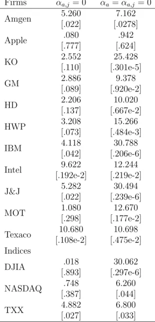
(19) the GARCH variance factor provides the main description of the smooth changes in daily volatility while jumps capture unusual episodes of volatility. This observation is born out in the descriptive statistics in Table V. Of particular interest is the average proportion of the conditional variance explained by the jumps which is about 20% for both IBM and Intel but 30% for Texaco and 40% for J&J. However, at times as much as 90% of the conditional variance for Amgen is due to the jump component.21 As previously noted, jumps will contribute to conditional skewness and kurtosis. Table V reports the average conditional skewness and kurtosis implied by the model. Even in the case of companies that have a relatively low number of jumps, the effects on higher conditional moments can be substantial. For instance, over the period 1990-1992 there is considerable variation in conditional kurtosis for Intel, reaching as high as 13 and spending most of the time in the range of 5 to 9. Equation 21 indicates that when λt > 0 the GARCH variance component will have an effect on conditional kurtosis, in contrast to a model without jumps which has a constant conditional kurtosis. A.1. The effect of jumps on expected volatility Traditional jump diffusion models assume the process governing jump arrivals is independently and identically distributed and do not allow jumps to affect the dynamics of diffusion volatility. In our case, jumps can affect expected volatility through two channels. Firstly, jumps affect the conditional variance directly through the time-varying Poisson arrival process and contribute to time variation in the second and higher-order moments. Secondly, the GARCH component of the conditional variance includes the propagation effects of previously realized jumps. Table VI summarizes statistical tests of whether or not jumps affect volatility dynamics. The first column of Table VI reports LR test statistics associated with the hypothesis that ρ = γ = 0. This test is designed to detect whether or not time-variation in the jump intensity contributes to expected volatility. As expected from the t-statistics associated with these parameter estimates in Table III, these LR test results strongly reject ρ = γ = 0 so that jump clustering affects the conditional variance through this channel. The results in the second column of Table VI refer to a LR test for the effect of jumps on conditional variance through GARCH feedback effects, that is, the propagation of previously realized jump innovations to expected volatility. If the parameters αj = αa,j = 0, then past jump innovations have the same effect on expected volatility as normal innovations. For all firms we reject this null hypothesis and conclude that jumps affect expected volatility differently than normal innovations. Therefore, jumps do affect the conditional variance through this channel, and as shown in columns 2 and 4 of Table VIII, tend to have a smaller positive feedback coefficient than do normal innovations. Recall that ²t−1 contains both normal and jump innovations that feedback into the GARCH component of volatility. The feedback coefficient g(·), associated with ²2t−1 in 21. Results available from the authors upon request.. 15.

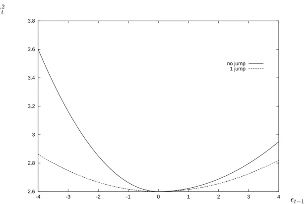
(20) the GARCH function, includes the extra term αj when good news and at least one jump occurs, and the extra terms αj + αa,j when a jump and bad news occurs. As reported in Table III, in 9 out of the 11 firms, αj < 0 reducing g(·) when a jump and good news occurs. Furthermore, when the news was bad and a jump occured, all firms experience a reduction in g(·) since αj + αa,j < 0. The implications for the size of g(·), which depends on the sign of the return innovation and also whether a jump was identified, are summarized in Table VIII. Although ²2t−1 is typically large after a jump, jumps result in a smaller g(·) than do normal innovations. This implies that news associated with jump innovations is incorporated more quickly into current prices. A.2. Asymmetries in the conditional variance Table VII evaluates the importance of asymmetric feedback from jump innovations in the presence of positive and negative return innovations. Except for Intel and Texaco, there is very little evidence (αa,j = 0) to suggest that the feedback from jump innovations to expected volatility is different in response to negative as opposed to positive return innovations (bad versus good news). This does not mean that jumps have no impact on expected volatility but instead tend to have a symmetric effect with respect to the type of news. The second set of test results in this table evaluate the hypothesis of no good vs bad news asymmetries when both jump and normal innovations are considered, that is, αa = αa,j = 0. Except for Amgen and Apple (p-values of .0289 and .624 respectively), we find asymmetry with respect to good and bad news measured by the total return innovation. These tests indicate that the traditional good vs bad news asymmetry is present when no jumps occur. Consider the IBM results as an example. The news impact curve for IBM is displayed in Figure 2. When no jumps occur, there is a clear asymmetry between good (²t−1 > 0) and bad (²t−1 < 0) news. However, when a jump occurs the news impact curve tends to flatten and become more symmetric. In terms of the parameter estimates in Table III, in the absence of a jump the coefficient associated with feedback from good news to to σt2 is exp(α) = .022, while the coefficient for bad news is greater, exp(α + αa ) = .063. When 1 jump occurred last period,22 the coefficient associated with good news is exp(α + αj ) = .014; while it is exp(α + αj + αa + αa,j ) = .016 for bad news. Table VIII reports the size of g(·) associated with these four cases for all firms. In summary, we find the traditional good and bad news asymmetry, but this appears to operate mostly when no jumps occur. In contrast, when jumps occur the usual good vs bad news effect diminishes in favor of a more symmetric effect on expected volatility. In addition, past jumps affect the conditional variance but they tend to have a smaller positive feedback coefficient than normal innovations. This evidence is consistent with the stylized fact that the persistence effect on expected volatility from large shocks to returns is often smaller than from normal innovations. 22. As inferred from the time t − 1 filter, E[nt−1 |Φt−1 ].. 16.

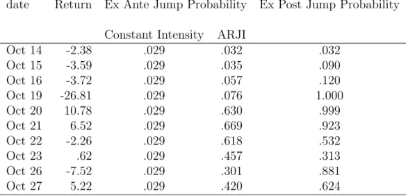
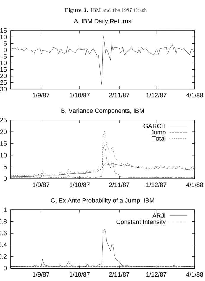
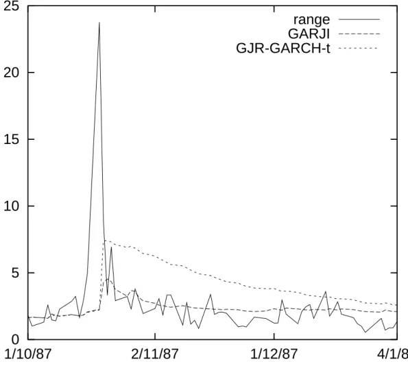
(21) A.3. Jump clustering around the 1987 crash Figure 3 focuses on the model for IBM around the 1987 crash. Panel B displays the conditional variance components of the model and indicates that it is the jump variance component that accounts for the effects on conditional variance after the crash. Notice that the smooth GARCH component of volatility shows very little increase after the crash. This is an important feature of jumps which is discussed in more detail below. Comparing panels C and D shows how poorly a constant jump intensity (λt = λ) version of the model does in capturing the jump dynamics for this period. Further evidence of the ability of the ARJI model to correctly identify and forecast jumps is seen in Table IX. This table compares the returns before and after the 1987 crash with the ex ante forecast of a jump from both the ARJI specification and the constant jump intensity version. The last column of this table reports the ex post probability of a jump.23 Using a criterion that a jump occurred if P (nt ≥ 1|Φt ) ≥ .5, we see that the ARJI specification provides a vast improvement over the constant jump intensity model in predicting jumps for this period. For example, the ARJI model identifies (ex post) the crash on Oct. 19 as a jump and forecasts (ex ante) the jumps that occur in the 3 days immediately following the crash, while the constant intensity probability of a jump is constant at .03 over the entire sample. To further investigate the ability of the GARJI specification to capture the volatility structure for IBM around the 1987 crash, Figure 4 presents a comparison of two conditional standard deviation forecasts (produced by alternative models) with a range-based measure of ex post volatility. Following Parkinson (1980),24 our estimate of the ex post daily standard deviation is √ ranget = κ log(Pt,h /Pt,l ) (25) where Pt,h and Pt,l are the intraday high and intraday low prices respectively, and κ is a parameter that was calibrated to the data to make the range estimate of the unconditional variance equal to the unconditional variance of daily returns.25 Figure 4 shows the standard deviation forecasts from our GARJI model, as well as those produced by a fat-tailed asymmetric GARCH model with no jumps. For the latter we use a GJRGARCH model with t-distributed innovations (GJR-GARCH-t). After the crash, the GJR-GARCH-t forecast completely overshoots realized volatility and persists at high levels for some time.26 In contrast, the GARJI reverts back to the lower actual levels of volatility much more quickly, and provides a superior forecast of daily volatility after the 1987 crash. 23. P (nt ≥ 1|Φt ) = 1 − P (nt = 0|Φt ). The estimator in Parkinson (1980) provides an efficient unbiased estimate of the volatility parameter from a geometric Brownian √ motion, but may be biased for other stochastic processes. 25 Parkinson (1980) set κ = .6 while we estimate it to be .74 for our sample. 26 The problem with the basic GJR-GARCH-t model is even clearer from Panel B of Figure 3 which shows the volatility components from the GARJI model. The GARCH variance component increases very little after the crash while most of the volatility dynamics are accounted for by the jump dynamics. 24. 17.

(22) A.4. Prescheduled earnings announcements Andersen and Bollerslev (1998b) showed that macroeconomic announcements which occur on predetermined dates are associated with a volatility component for exchange rates that can have large but generally short-lived effects. In our context, although earnings surprises are only one source of jumps, it might be important to differentiate between jumps on prescheduled earnings announcement days versus jumps on days when there was unscheduled news. For our historical samples for IBM and Intel, approximately 16% and 23% of jumps were associated with prescheduled earnings announcement days. That is, using our model’s filter and the criterion that at least one jump occurred on day t if P (nt ≥ 1|Φt ) ≥ .5, for Intel we identify jumps on 62 days, of which 14 coincide with days when there was an earnings announcement (or the day after if the announcement was after the market closed). For IBM, jumps occurred on 145 days, 24 of which were earnings announcement days.27 On the other hand, only 20% of scheduled earnings announcements result in jumps. To investigate whether or not prescheduled earnings announcements have different effects than other sources of jumps, we explored a parameterization which allows an earnings announcement day dummy variable to affect the jump intensity as well as the GARCH conditional variance. We tried several specifications, including allowing the effect of the dummy to propagate versus allowing for a one-time only effect on the conditional intensity and GARCH variance. We found that the one-time effect provided the best loglikelihood value. Note that the earnings announcement dummy variable was turned on for both the day of the announcement and the day after due to the fact that many announcements occur after the market closes. The results for this richer model are very comparable to our main results which were discussed above and reported in Table III. In particular, all of our conclusions, such as jump clustering and volatility asymmetries, are robust to the addition of prescheduled announcement dummies. The effect of announcement dummies was imprecisely estimated for our data. As noted above, the relatively infrequent occurrence of announcements that result in jumps, mean that long samples are needed to accurately identify different types of jump dynamics.. B. Indices During discussion of the results for individual firms, it appeared as if there might be differences between traditional firms and new economy firms. Given that available timeseries are too short for many internet stocks, and also that it is difficult to classify some firms as traditional versus high-tech, this section reports results for our GARJI model applied to three different indices which cover different types of firms. Table X reports 27. We have IBES data on earnings announcement days starting in the third quarter of 1971 which covers three quarters of our total sample for IBM.. 18.

(23) parameter estimates for the GARJI model for the DJIA, NASDAQ 100 and the CBOE Technology Index (TXX). The specification of the GARJI model in this table includes an AR(1) term to account for the autocorrelation found in the conditional mean of returns for the indices.28 The three indices cover the spectrum of volatility levels from low to high, ordered as DJIA, NASDAQ 100, and TXX. Unconditional standard deviations are .948, 1.815 and 2.429 for the DJIA, NASDAQ and TXX respectively. Consistent with this ordering is an increased likelihood of jumps for the more volatile indices. For instance, the implied unconditional jump intensities are .135, .136 and 1.429 for the DJIA, NASDAQ 100 and TXX, respectively. The average variance due to jumps is .224 (DJIA), .443 (NASDAQ 100), and 5.073 (TXX). The more volatile the index the larger the jump variance, although the proportion of the conditional variance explained by jumps is still quite low overall, .166 for the DJIA, .144 for the NASDAQ 100, and .228 for the TXX index. These results suggest that jumps in the DJIA are less frequent and have a smaller effect on returns than the other indices. Conversely, returns from the volatile TXX index display frequent large jumps. There are several features that are common for individual firm and index dynamics. For both, the addition of the ARJI jump dynamics provides a strong statistical improvement over a constant jump intensity specification (see estimates for ρ and γ in Table X and column 1 of Table VI). The process governing the arrival of jumps is serially correlated which implies jump clustering for the indices as well. One difference between the individual firm results and those for the two most volatile indices is that revisions to the conditional jump intensity, ξt−1 , are more important for the latter. For example, γ is .936 and .974 for the NASDAQ 100 and TXX respectively, which is larger than the value for the DJIA and all the individual firms. The final 3 rows in Table VI and Table VII report the LR test results for the effect of jumps on expected volatility for the indices. In each case, jump effects on conditional variance are important. The first column of Table VI shows that the time-varying jump intensity will affect expected volatility for all indices. The second column shows that jump innovations have a different feedback on expected volatility than do normal innovations (this differential is weakest for the TXX which is the smallest dataset and may not contain sufficient information to identify this aspect of the model). Like the individual firm results, the feedback coefficient, g(·), tends to be smaller when a jump innovation is part of the return innovation. For instance, for the DJIA, the feedback coefficient associated with good news and no jumps is g(·) = exp(α) = .014, but exp(α + αj ) = .007, when one jump occurred. Also, in common with the results for individual firms, the last three rows of the first column of Table VII show that there is no evidence of asymmetric jump feedback (ie. αa,j = 0) with respect to good or bad news. However, at least for the DJIA index, the final column of Table VII indicates that bad news asymmetries are still important for normal innovations in the absence of a jump. 28. Market microstructure effects such as stale prices can cause low-order autocorrelation in index returns.. 19.

(24) A direct result of jumps is that they can cause significant conditional and unconditional skewness (see Equation 20). Conditional skewness is affected by the magnitude and sign of θ. The jump size mean, θ, is significantly negative for all three indices while it is centered around zero for most firms (the exception is Texaco). This indicates that a negative time-varying conditional correlation between jump innovations (consequently return innovations) and squared return innovations is an important feature of the indices.29 These results are consistent with a time-varying leverage effect in which large negative return realizations, in this case due to jumps, are associated with an immediate increase in the variance. This result of a significant contemporaneous asymmetry is associated with a weaker asymmetry between the sign of lagged innovations and the GARCH variance component for the indices as compared to the individual firms.30 This is consistent with Duffee (1995) who reports a significant negative contemporaneous correlation between aggregate stock returns and volatility but a weaker contemporaneous correlation for individual stock returns and volatility. Duffee (1995) speculates that there is a negatively skewed market factor and an idiosyncratic firm factor which is positively skewed. We conclude that for the indices a time-varying contemporaneous leverage effect which is captured by jumps is more important than the lagged leverage effect which is identified in the GARCH structure.. V. Evaluation of Variance Forecasts This section summarizes results from our evaluation of the out-of-sample forecasts from our GARJI model as compared to a benchmark GJR-GARCH-t model. In all cases, we re-estimated the models reserving 1500 observations for the out-of-sample analyses. Conditional variance forecasts were based on these estimates and the parameters were updated (re-estimated) every 50 observations. One frequently used method to evaluate forecasts is to run a linear regression of the realized variable on its forecast. Then the coefficient of determination, R2 , provides a measure of the value of the forecasts. In the case of volatility this is complicated by the fact that the target is unobservable. Traditional proxies for ex post volatility, such as squared daily returns, are noisy and relatively ineffective for discriminating among forecasting models. Andersen and Bollerslev (1998a) show that the use of intraday prices can provide improved ex post estimates of latent volatility. One such estimator is the range, Equation 25, which was used in the previous section to compare volatility forecasts for IBM around the 1987 crash. Therefore, we evaluate our out-of-sample volatility forecasts using the R2 from the following regression, ranget = a + bVart−1 (rt )1/2 + errort (26) 29. Covt−1 (²t , ²2t ) = Et−1 ²3t < 0 if θ < 0. Applying the benchmark GJR-GARCH-t model to the indices revealed significant asymmetries but in the GARJI model these feedback asymmetries are diminished. Results are available on request. 30. 20.

(25) where ranget is the estimate of the ex post standard deviation on day t, and Vart−1 (rt )1/2 is the square root of the out-of-sample conditional variance forecast for day t from a particular model.31 A higher R2 implies a better forecasting model in the sense that a larger percentage of the variability of realized volatility is explained by that model’s forecasts. The first row of results in Table XI reports the R2 from the forecast evaluation regression (26) for the GJR-GARCH-t and the GARJI models applied to all firms.32 With the exception of Texaco, the GARJI produces a higher out-of-sample R2 for all firms, although the models are about equal for Amgen. In some cases, the improvement in the R2 from the GARJI model is substantial (Apple, HD, HWP, IBM, and MOT). The Texaco exception is interesting since we found that case to be different from other firms in several respects, notably a higher average intensity of jumps and a significantly positive jump-size mean. Although the GARJI model appears to add little to volatility forecasts for Texaco, the strong rejection of a constant intensity specification reported in Table VI suggests the GARJI dynamics may improve other features of the return distribution, such as density forecasts. The second panel of results conditions on the observations of higher than normal volatility, that is, including observations in (26) only when the ranget is greater than its mean plus one standard deviation. The ranking of the models is consistent with the results reported in the first panel which used all of the out-of-sample data. The GJR-GARCH-t benchmark model can capture volatility clustering and fat-tails. However, since that model is from the location-scale family of distributions, the shape of the tails of the return distribution remain constant over time.33 On the other hand, the GARJI model is an example of a time-varying mixture of distributions which allows the shape of the tails of the return distribution to change over time. Therefore, the more flexible GARJI model should be able to capture dynamics in the tails of the return distribution, particularly after a large price move. In Section IVA.3 we illustrated the improved forecasts of the GARJI model after the 1987 crash for IBM. This suggested that the addition of jump dynamics plays an important role in improving forecasts after a large negative move in the market. Again, the important question is whether our richer specification also performs better for out-of-sample forecasts. To investigate this for all firms, we consider another conditional regression evaluating out-of-sample forecasts using data around large negative returns. In particular, we condition on the daily return being less than -2% and include the 10 days immediately following this 31 We also evaluate conditional variance forecasts using the square of the range as our target value. The ranking of the models is identical to the results based on Equation (26). 32 As noted in Section IVA.3, the unadjusted range statistic is a biased measure of the ex post standard deviation and also, due to Jensen’s inequality, the square root of the variance forecast will be a biased measure of the conditional standard deviation forecast. Our focus is not on potential bias of the model forecasts but on their ability to explain changes in the volatility as measured by the R2 from regression (26). 33 For example, the conditional skewness and kurtosis are constant over time for the GJR-GARCH-t model.. 21.

(26) downward move in the market. The R2 s from the regression (26) associated with the out-of-sample forecasts for these episodes in our sample are reported in the bottom panel of Table XI. As expected, the predictive ability of both models declines compared to the top row which includes all of the data, but the GARJI specification continues to provide superior forecasts compared to the GJR-GARCH-t alternative for 10 out of 11 firms. In summary, the results in the three panels of Table XI show that the GARJI model produces superior forecasts relative to a benchmark GJR-GARCH-t model. These results include out-of-sample forecasts for average volatility, above average volatility and the volatility just after large negative moves in the stock price. These substantial improvements in the out-of-sample forecasts, relative to a popular benchmark model, should facilitate improved financial management decisions.. VI. Summary In this paper we have developed a model of the components of the return distribution implied by the impact of different types of news. We interpret the innovation to returns, which is directly measurable from price data, as the news impact from latent news innovations. The latent news process is postulated to have two separate components, normal and unusual news events, which have different impacts on returns, expected volatility, and higher-order moments of the return distribution. Normal news innovations are assumed to cause smoothly evolving changes. The second component of the latent news process causes infrequent large moves in returns which we label jumps. Therefore, the latent news process induces two separate components governing the distribution of returns. The volatility process is affected by both components driving returns. The conditional variance of the normal innovation captures the smooth autoregressive component in volatility; whereas the conditional variance of the jump innovation captures unusual and often extreme price movements from significant information events. The intensity of the jump process is explicitly modeled as a serially correlated conditional Poisson process. This time-varying intensity affects volatility dynamics directly. In addition, previous jump innovations feedback into expected volatility through the GARCH component of conditional variance. Furthermore, normal and jump innovations have potentially asymmetric effects on volatility dynamics. This rich specification allows for conditional contemporaneous leverage effects and lagged leverage effects. These features extend traditional models that combine GARCH and SV with jumps. In summary, we find evidence of time dependence in jump intensities for both individual stocks and indices using an autoregressive conditional jump intensity parameterization; allow jump innovations to feedback to expected volatility; provide new results on asymmetric effects of return innovations on volatility; and find evidence of a time-varying contemporaneous leverage effect. These novel features allow jumps to have different impacts, feedbacks and decay rates as compared to normal innovations allowing the model to perform better around crash periods and other events in the tail of the distribution. 22.