HAL Id: tel-01483770
https://hal-lirmm.ccsd.cnrs.fr/tel-01483770
Submitted on 6 Mar 2017
HAL is a multi-disciplinary open access
archive for the deposit and dissemination of sci-entific research documents, whether they are pub-lished or not. The documents may come from teaching and research institutions in France or abroad, or from public or private research centers.
L’archive ouverte pluridisciplinaire HAL, est destinée au dépôt et à la diffusion de documents scientifiques de niveau recherche, publiés ou non, émanant des établissements d’enseignement et de recherche français ou étrangers, des laboratoires publics ou privés.
Swan Rocher
To cite this version:
Swan Rocher. Querying Existential Rule Knowledge Bases: Decidability and Complexity. Artificial Intelligence [cs.AI]. Université de Montpellier, 2016. English. �tel-01483770�
D´
elivr´
e par l’Universit´
e de Montpellier
Pr´
epar´
ee au sein de l’´
ecole doctorale I2S
Et de l’unit´
e de recherche UMR 5506
Sp´
ecialit´
e: Informatique
Pr´
esent´
ee par Swan Rocher
Querying Existential Rule
Knowledge Bases:
Decidability and Complexity
Soutenue le 25 novembre 2016 devant le jury compos´e de : Directrice de th`ese
Mme. Marie-Laure Mugnier Professeur Univ. de Montpellier
Co-encadrant
M. Jean-Fran¸cois Baget Charg´e de Recherche INRIA
Rapporteurs
Mme. Marie-Christine Rousset Professeur Univ. de Grenoble
M. Sebastian Rudolph Professor Univ. Dresden
Examinateurs
M. Christophe Paul Directeur de Recherche CNRS
Remerciements
Trois ans, c’est court, et pourtant c’est en ´ecrivant ces remerciements que je me rends compte que j’ai eu l’occasion de rencontrer ´enorm´ement de gens, qui m’ont tous apport´e quelque chose plus ou moins directement, si bien qu’il est difficile d’ˆetre sˆur de n’oublier personne...
Merci tout d’abord `a Jean-Fran¸cois et Marie-Laure pour avoir ´et´e des directeurs de th`ese parfaits ! Tant au niveau scientifique que personnel, vous avez toujours ´et´e l`a lorsque j’en avais besoin.
Bien sˆur, merci aussi `a Marie-Christine Rousset et Sebastian Rudolph pour votre lecture si attentive de ce manuscrit : ma th`ese ne serait pas ce qu’elle est sans vos remarques. Merci ´egalement `a Andreas Pieris et Christophe Paul pour avoir accept´e d’ˆetre examinateurs, et merci aussi `a Christophe pour avoir particip´e `a mon comit´e de suivi de th`ese ces trois ans !
On s’´eloigne un petit peu, mais pas trop, merci `a Michel et le projet Qualinca, sans qui je n’aurai pas pu faire cette th`ese. Merci Annie pour avoir r´eussi `a garder ton calme malgr´e ma hantise des d´emarches administratives. Et merci `a toute l’´equipe, ses permanents, ses stagiaires et bien sˆur ses doctorants (pass´es et actuels), Micha¨el pour tes conjectures et tes contre-exemples, Stathis pour tes questions existentielles, L´ea pour tes histoires `a base de chats et/ou lapins, et tous les autres !
Non doctorant, mais c’est comme si, merci beaucoup Cl´ement, co-bureau `a travers les ages, pour les discussions du caf´e, et pour tout le reste d’ailleurs !
On peut porter le regard un peu plus loin car le LIRMM n’est pas seulement une ´equipe. Merci `a tous les gens avec qui j’ai pu discuter au d´etour d’un couloir ou autour d’un caf´e. En particulier, merci beaucoup `a Sabrina, Ana¨el, Guilhem, Valentin, Julien, Fran¸cois, Florian, Jessie et Nam’ `a la fois pour la d´etente, et pour les moments scientifiques. Ces ann´ees n’auraient certainement pas ´et´e les mˆemes sans votre pr´esence ! Non, je ne t’oublie pas, merci Chlo´e pour m’avoir aid´e `a en arriver l`a ! Et merci Marthe pour ton th´e parfaitement ´equilibr´e et tes nombreux gˆateaux !
Finalement, le LIRMM ne serait pas ce qu’il est sans Laurie et Nicolas : toujours souriants, et on ne peut plus efficaces, merci beaucoup pour tout ce que vous avez fait !
Plus loin que Montpellier (beaucoup), merci `a Charlotte et Julien pour m’avoir accueilli dans un super paysage quand il fallait que je me change les id´ees ! Je n’oublierai pas mon “bureau” `a la montagne.
Enfin, il est plus que temps de remercier la famille : merci Luc et Sarah pour votre soutien et n’avoir jamais dout´e. Et bien entendu merci pour tout Eva ! Il me semble aussi important de remercier la famille un peu moins directe : alors, merci Raphy pour ton accueil, et aussi pour la force de volont´e que tu m’as apport´e d’ailleurs. Merci ´egalement `a Lyes, malgr´e tes blagues douteuses, tu m’as permis de rigoler quand je ne m’y attendais pas ! Et ´evidemment, merci `a Sandie pour m’avoir support´e pendant la r´edaction de cette th`ese !
Contents
1 Fundamental Notions 7
1.1 General Mathematical Notions . . . 7
1.1.1 Basic Notations . . . 7
1.1.2 Graph Notions . . . 8
1.1.3 Logical Notions . . . 9
1.1.4 Complexity Classes . . . 11
1.2 Existential Rule Framework . . . 11
1.2.1 Forward Chaining . . . 16
1.2.2 Backward Chaining . . . 18
1.3 Some Useful Translations . . . 21
2 Landscape of Decidable Classes of Rules 25 2.1 Abstract Rule Classes . . . 25
2.2 Finite Expansion Set . . . 28
2.3 Bounded Treewidth Set . . . 33
2.4 Finite Unification Set . . . 37
2.5 Description Logics . . . 43
2.6 Kiabora . . . 46
3 Acyclicity Conditions for Chase Termination 47 3.1 Different kinds of chase . . . 48
3.2 Acyclicity notions . . . 56
3.2.1 Dependency-based Approach . . . 57
3.2.2 Position-based Approach . . . 59
3.2.3 First combination . . . 64
3.3 Unifying both Approaches . . . 65
3.4 Extensions . . . 78
3.5 Other Acyclicity Conditions . . . 86
3.5.1 Model Summarizing Acyclicity and Model Faithful Acyclicity . 86 3.5.2 Extending Model Summarizing Acyclicity . . . 90
4 Combining Transitivity and Decidable Classes of Existential Rules 93
4.1 Transitivity and BTS/FES rules . . . 94
4.1.1 Overview of Known Results . . . 94
4.1.2 A General Undecidability Result . . . 97
4.1.3 Clarifying the FES Landscape . . . 98
4.2 Linear Rules and Transitivity . . . 101
4.2.1 Framework . . . 101
4.2.2 Overview of the Algorithm . . . 107
4.2.3 Rewriting Steps . . . 108
4.2.4 Termination and Correctness . . . 118
Introduction
Querying Knowledge BasesThe recent years have been marked by a tremendous increase of the volume and the heterogeneity of available data sometimes referred to as the “data deluge”. Exploit-ing these data has become a major issue in several research domains (knowledge representation and reasoning, data management, Semantic Web, ...) and the need for integrating data semantics into querying mechanisms has been widely acknowl-edged. This has renewed the interest for ontologies, which are typically used to formalise general background knowledge on the modeled domains.
Indeed, ontologies have several qualities with respect to better exploiting data: • they can be used to integrate heterogeneous data from different sources by
providing a common vocabulary;
• they allow to adapt the querying vocabulary to specific users’ needs, hence abstracting from how data are actually stored;
• they allow to infer knowledge that is not explicitly stored in the data, hence palliating incompleteness in the data.
However, taking into account data semantics requires both suitable ontologi-cal formalisms and new query answering mechanisms able to integrate ontologiontologi-cal knowledge. Indeed, classical query answering mechanisms have been tailored and optimised for databases. Now, the focus has been shifted to knowledge bases, in which an ontological layer is added on top of data.
This motivated a new research line that led to proposals known as Ontology-Based Data Access (OBDA, e.g., [CDL+07, PLC+08]), Ontological Query Answer-ing (e.g., [CGP11, Mug11]) or Ontology-Mediated Query AnswerAnswer-ing (OMQA, e.g., [BO15, Bie16]). In these approaches, the ontological layer is seen as a logical theory in (a fragment of) first-order logic and data are abstracted into logical facts (which can be mapped to actual data).
Existential Rules
These new issues have deeply influenced research in Description Logics, the major family of formalisms to represent and reason with ontologies [BCM+03]. This led
to the definition of new description logics, generally called lightweight description logics, such as the DL-Lite [CDL+07] and the E L [BBL05] families, as well as the associated profiles of the Semantic Web language OWL 2. At the same time, a new logical framework has emerged, called existential rules [BLMS11, KR11], also known as Datalog+/- [CGL12]. Existential rules have a double origin: on the one hand, they were designed as an extension of Datalog, the language of deductive databases [AHV95], for ontological representation purposes, hence the name Datalog+/-; on the other hand they correspond to the logical translation of rules in a graph-based knowledge representation framework [CM09]. They also have the same form as high-level constraints from the database theory, known as Tuple Generating Dependencies (TGDs) [BV84]; note however that TGDs define constraints on the data, while existential rules are used to infer knowledge on the data. Finally, it appears that the existential rule framework generalises most of the new description logics developed for querying data.
More precisely, existential rules are positive and conjunctive rules of the form “if body then head ”, with a specific feature: it is possible to introduce in the head of a rule variables that do not occur in the body. These variables are existentially quantified. Thanks to this particularity, existential rules are able to infer the ex-istence of individuals not necessarily present in the initial data. This makes them well-adapted to open-world reasoning, in which not only we cannot assume that only what is explicitly encoded in the data is true, but also in which we cannot suppose that the only known objects are those present in the data. Such a feature is considered important for representing and reasoning with ontological knowledge. Let us illustrate this with a simple example. Consider two roommates Bob and John, and assume we know that John pays for Internet. We can see these data as a set of facts roommates(Bob, J ohn) ∧ paysInternet(J ohn). We now want to know if Bob has Internet at home and so we ask the query ∃x(livesIn(Bob, x) ∧ hasInternet(x)). Without ontological knowledge we are not able to answer posi-tively. Despite, we intuitively would like to answer yes: some ontological knowledge is missing to get a positive answer. First, we know that if two persons are roommates, there is some place where they both live, hence the rule ∀x∀y(roommates(x, y) → ∃z(livesIn(x, z) ∧ livesIn(y, z))). We also want to say that if someone pays for Internet and lives somewhere, then Internet is present in that “somewhere”, which we formalise by the rule ∀x∀y(livesIn(x, y) ∧ paysInternet(x) → hasInternet(y)). Now our query gets a positive answer, indeed Bob and John, being roommates, live in the same place. John pays for Internet, hence he gets Internet at home. There-fore, Bob lives in a place where there is Internet. We could even add some other rules to complete the background knowledge of this example, for instance, we could say that roommate is a symmetrical relation, which we could express with the rule ∀x∀y(roommates(x, y) → roommates(y, x)).
Existential rules have the simplicity of rule-based languages, a privileged form to express human knowledge, as well as their flexibility, i.e., they are able to adapt to various kinds of data and are easily extended to encode new information. While
3
being simple, they are highly expressive, which allows to encode various kinds of ontological knowledge. Unsurprisingly, this expressivity has a cost: indeed, most reasoning problems over existential rules knowledge bases are undecidable (e.g., from [BV81] on TGDs). This motivated intense research in the last years to find classes of rules for which reasoning is decidable and hopefully tractable. Currently, a large landscape of decidable classes is known with different expressivity-complexity trade-offs.
This thesis makes further contributions to the study of decidable existential rule classes and to the analysis of their complexities.
Contributions of this Thesis
We consider knowledge bases in which the ontology is a set of existential rules. About the queries, we consider conjunctive queries, which can be seen as existentially quan-tified conjunctions of atoms. These queries correspond to the basic and most used queries in databases. Hence, the fundamental problem we study is the conjunctive query entailment problem (CQ entailment), which asks whether a conjunctive query is entailed by a knowledge base.
Our contribution is twofold. First, we analyse the different “acyclicity-based” decidable rule classes found in the literature. These rule classes rely on acyclicity conditions to ensure the finiteness of some forward chaining algorithm. We propose a tool that allows us to unify most acyclicity notions and to extend them in generic way. We also analyse the complexity of the recognition problem, i.e., deciding whether a given set of existential rules satisfies these new acyclicity notions. The main paper associated with this work is [BGMR14a].
Second, we consider the decidability (and complexity) of the CQ entailment problem when combining known decidable rule classes with a frequently required construct in ontological modeling, namely the transitivity of binary relations. We clarify the decidability picture for all the (currently known) classes for which some forward chaining algorithm halts. Then, we study the particular case of linear existential rules, and show that, up to a minor safety condition, linear rules are compatible with transitivity. We finally consider the complexity of the CQ entail-ment problem over knowledge bases composed of (safe) linear and transitivity rules. Most of this work is reported in [BBMR15], however, with respect to that paper, we provide a new undecidability result and correct a flaw in a complexity proof.
Other Contributions
During these three years, we have also considered other issues related to existential rules. The results obtained are not detailed in this thesis, hence we briefly mention them below, and refer the interested reader to the associated papers.
Our work on acyclicity-based decidable classes of rules was also motivated by the objective of extending decidable cases of CQ entailment for existential rules extended with a particular nonmonotonic negation, namely stable negation. Briefly, adding nonmonotonic negation to existential rules allows to apply rules only if some negated atoms from the rule body are not entailed by the knowledge base. While it is easy to see that stable negation may complicate the design of algorithms and increase the complexity of the CQ entailment problem, it also appears that it may make this problem undecidable, even when stable negation is added to a decidable class of positive existential rules. We have thus proposed a way to extend the results obtained for acyclicity-based positive existential rules to existential rules with stable negation. This work has been published in [BGMR14b].
Another interesting issue is how to deal with inconsistent knowledge bases. In this thesis, we assume that knowledge bases are consistent, but in practice, there are reasons to believe that it is not a safe assumption. Indeed, in a world where such a volume of data is available, which furthermore come from different data sources, it is likely that inconsistencies arise. From a logical point of view, an inconsistent knowledge base allows to infer everything, and in the context of querying data, it is obviously not the desired behaviour. We focus on the case where the ontol-ogy is assumed to be consistent, hence inconsistencies in the knowledge base come from the data (which is the most considered setting). When it is not possible to effectively repair the data, one has to consider query mechanisms tolerant to incon-sistencies. Various inconsistency-tolerant semantics have been defined, which all rely on a common idea: answers to queries are drawn from some maximally consistent subsets of the data (possibly added with some consistent inferred knowledge), called repairs. We have taken part in the definition of a general framework that unifies most inconsistency-tolerant semantics from the literature [BBB+16a]. Briefly, this
framework sees an inconsistency-tolerant semantics as a pair, composed of a “modi-fier” of the inconsistent knowledge base that allows to select some maximal repairs, and an “inference-strategy” that allows to infer conclusions from these selected re-pairs. Concerning the notion of maximal consistent subset, at least two different measures can be interesting: maximality in terms of set inclusion and maximality in terms of cardinality. The inference strategy may want to find an answer in all selected repairs, in their intersection, in a single one, or in a majority of them. These choices give rise to different semantics, some of them corresponding to existing pro-posals, while others are new. Our specific contribution in the context of this general framework consisted in analysing the data complexity of the obtained semantics for the fus subset of existential rules, which generalises most members of the DL-Lite family [BBB+16b].
Finally, we have also developed Kiabora, a software tool that allows to recognise most known decidable rule classes and proposes ways of combining them [LMR13]. The first version of this tool is available via a web interface at www.lirmm.fr/
5
kiabora. The second version has been integrated into the toolkit Graal dedicated to querying knowledge bases within the existential rule framework. Graal provides an abstract layer that allows to store and query various kinds of data (relational databases, RDF triple stores, internal memory, ...), forward and backward chaining algorithms, as well as complementary tools such as Kiabora and translators from or to other languages. More information can be found on Graal website at http: //graphik-team.github.io/graal/. Beside the development of Kiabora itself, we have helped to design and implement part of Graal [BLM+15, BGL+15].
Organisation of the Thesis
The remainder of this thesis is organised in as follows.
In Chapter 1, we define required mathematical notions and introduce the ex-istential rule framework. We recall various well-known results that we will use throughout the manuscript.
In Chapter 2, we present an overview of the main rule classes for which the CQ entailment problem is decidable. We first recall three abstract rule classes that ensure a specific behaviour of some reasoning algorithms. These classes are abstract in the sense that the associated recognition problem is undecidable. Then we review the main known concrete decidable rule classes, which are obtained by enforcing some syntactic restrictions on the sets of rules. Most of them belong to one or more abstract rule classes.
Chapter 3 is devoted to decidable rule classes that rely on acyclicity condi-tions ensuring the halting of some forward chaining variant, also known as chase in database theory. The first part of this chapter is dedicated to the main known chase variants, for which we give a unified formal definition. We then detail acyclicity-based rule classes, which rely on different graphs. We propose a way to unify these different acyclicity notions with a new graph and associated notion of dangerous cycles. Finally, thanks to the tool we used to unify them, we extend previous acyclicity-based rule classes.
In Chapter 4, we are interested in combining the transitivity of binary relations with known decidable rule classes. We first review known results on this issue obtained in the context of existential rules. Then, we provide new undecidability results, which allows to clarify the picture for rule classes for which some forward chaining algorithm halts. Finally, we consider the case of linear existential rules, one of the simplest, yet useful, classes of existential rules. We show that, up to a minor safety condition, linear and transitivity rules are compatible, and provide complexity results for the CQ entailment problem in terms of data and combined complexity.
Finally we summarise our contributions and outline further research in the con-clusion.
Chapter 1
Fundamental Notions
Contents
1.1 General Mathematical Notions . . . 7
1.1.1 Basic Notations . . . 7
1.1.2 Graph Notions . . . 8
1.1.3 Logical Notions . . . 9
1.1.4 Complexity Classes . . . 11
1.2 Existential Rule Framework . . . 11
1.2.1 Forward Chaining . . . 16
1.2.2 Backward Chaining . . . 18
1.3 Some Useful Translations . . . 21
1.1
General Mathematical Notions
In this section we define several basic mathematical notions and notations needed in this thesis.
1.1.1
Basic Notations
Given a function f , we denote by dom(f ) the domain of f . If we are also given a set X, we denote the restriction of f to X by f |X = {(x, f (x)) | x ∈ dom(f ) ∩ X}.
A sequence S is a function whose domain is N if it is infinite, ∅ if it is of length 0, and {0, . . . , n − 1} if it is of length n ∈ N+. We denote by S
i the ith element of
S, i.e., Si = S(i).
1.1.2
Graph Notions
Given a (hyper)graph G, we denote by V (G) its set of vertices and E(G) its set of (hyper)edges. A (hyper)graph can be either directed or undirected, in the for-mer case edges are ordered, while in the latter they are not, i.e., in an undirected (hyper)graph, edges (x, y) and (y, x) are the same object.
Given a directed graph G and a vertex v ∈ V (G) we denote its neighbourhood in G by Γ(v) = {x | (v, x) ∈ E(G)}.
Definition 1.1 (Path)
Given a graph G, a path is a sequence of edges (x1, x2), . . . , (xk−1, xk) such that
for all 1 ≤ i < k, (xi, xi+1) ∈ E(G).
If G is directed we say that the path is from x1 to xk (and we say that xk is
reachable from x1). If G is undirected we say that the path is between x1 and xk.
Now can be defined the notion of a connected component in an undirected graph. Definition 1.2 (Connected Component)
Given an undirected graph G, a connected component of G is a subset C ⊆ V (G) such that for any u, v ∈ C, there is a path between u and v.
This notion has been extended to strongly connected components for directed graphs as follows.
Definition 1.3 (Strongly Connected Component)
Given a directed graph G, a strongly connected component of G is a subset C ⊆ V (G) such that for any u, v ∈ C there is a path from u to v (i.e., v is reachable from u).
In Chapter 2, we also use the notion of treewidth of a (hyper)graph. This notion relies on the notion of tree decomposition defined next.
Definition 1.4 (Tree Decomposition)
A tree decomposition T of a hypergraph G, is a tree where each vertex t is labelled by a set of vertices (also called bag) λ(t) ⊆ V (G) such that:
• ∀u ∈ V (G), ∃t ∈ V (T ) such that u ∈ λ(t); • ∀e ∈ E(G), ∃t ∈ V (T ) such that e ⊆ λ(t);
• ∀u ∈ V (G), ∀ti, tj ∈ V (T ) such that u ∈ λ(ti) and u ∈ λ(tj), for all tk in the
only path between ti and tj in T , u ∈ λ(tk).
Then, from a tree decomposition, one can compute its “width”, which is the maximal size of one of its bags (minus one).
1.1. GENERAL MATHEMATICAL NOTIONS 9
Definition 1.5 (Width)
Given a tree decomposition T , the width of T is defined as width(T ) = max
t∈V (T )|λ(t)| − 1
.
Finally, the treewidth of a (hyper)graph is the minimal width of one of its tree decompositions.
Definition 1.6 (Treewidth)
Given a (hyper)graph G, its treewidth is defined as the minimal width among all tree decompositions of G.
This notion is quite useful as it helps to measure the distance between a graph and a tree, for instance, trees have treewidth one, cycles have treewidth two, and if a graph contains a clique of size k then its treewidth is at least k − 1.
1.1.3
Logical Notions
A logical language L = (P, C) is a pair composed of a finite set of predicates P and a (potentially infinite) set of constants C. Furthermore, we are given an infinite set of variables V. With each predicate of P is associated a non-negative integer called its arity. We do not consider functional symbols except for constants (which are functional symbols of arity 0).
Then, a term of L is either an element of C (thus a constant), or a variable from V. An atom of L is of the form p(t1, . . . , tk) where p is a predicate from P of arity
k, and t1, . . . , tk are terms from L. It is a ground atom if all its terms are constants.
For brevity reasons, we sometimes use the expression p-atom to denote an atom with predicate p.
Given an atom α, we denote by terms(α) the set of all terms in α, by var(α) the set of all variables in α and by const(α) the set of all constants in α.
In our examples, we denote variables by letters from the end of the alphabet (x,y,z,u,...), and constants by letters from the beginning of the alphabet (a,b,c,...). Definition 1.7 (Interpretation)
An interpretation of a logical language L = (P, C) is a pair I = (D, I) where D is a non-empty set called the interpretation domain and where I is an interpretation function of the symbols of L such that:
• for any c ∈ C, I(c) ∈ D;
• for any p ∈ P of arity k, I(p) ⊆ Dk.
An interpretation of L is a model of a formula built on L if it makes this formula true by considering the classical interpretation of logical connectives and quantifiers.
Definition 1.8 (Logical Consequence, Equivalence)
Given a language L and two formulae φ1 and φ2 on L, φ2 is a (logical) consequence
of φ1, which is denoted by φ1 |= φ2, if all models of φ1 are models of φ2.
If φ1 |= φ2 and φ2 |= φ1, φ1 and φ2 are (logically) equivalent, which is denoted
by φ1 ≡ φ2.
Definition 1.9 (Substitution)
Given a set of variables X and a set of terms T , a substitution σ of X by T is a mapping from X to T .
Given an atom α, we denote by σ(α) the atom obtained by substituting each occurrence of x ∈ var(α) ∩ X by σ(x), i.e., if α = p(t1, . . . , tk) then σ(α) =
p(σ(t1), . . . , σ(tk)).
Given a set of atoms A, σ(A) denotes the set obtained by applying the substitution on each atom, i.e., σ(A) = {σ(α) | α ∈ A}.
Definition 1.10 (Homomorphism and Isomorphism)
Given two sets of atoms A1 and A2, a homomorphism from A1 to A2 is a
sub-stitution π of var(A1) by terms(A2) such that π(A1) ⊆ A2. In this case we say that
A1 maps to A2 by π.
If π is injective (thus π−1 is a function) and π−1 is a homomorphism from A2 to
A1, π is an isomorphism from A1 to A2.
An isomorphism can also be defined as a bijective substitution σ from var(A1)
to var(A2) such that σ(A1) = A2. That is why it is often called a “bijective variable
renaming”.
Furthermore, homomorphisms can also be defined for interpretations. Definition 1.11 (Homomorphism between Interpretations)
Given two interpretations I1 = (D1, I1) and I2 = (D2, I2) of a logical language
L = (P, C), a homomorphism from I1 to I2 is a mapping π from D1 to D2 such
that:
• for all c ∈ C, π(I1(c)) = I2(c),
• for all p ∈ P and (t1, . . . , tk) ∈ I1(p), (π(t1), . . . , π(tk)) ∈ I2(p).
The last basic logical notion we need is that of prenex form. Definition 1.12 (Prenex Form)
A first-order logical formula is in prenex form, if it is written as a sequence of quantifiers followed by a formula without quantifier, and such that the scope of each quantifier is the whole formula.
It is well known that every first-order formula can be rewritten into a first-order formula of prenex form. Hence, in the following we always assume that all formulae we are dealing with are under prenex form, which allows us to simplify the various definitions and proofs.
1.2. EXISTENTIAL RULE FRAMEWORK 11
1.1.4
Complexity Classes
In this thesis we make use of several complexity classes. While we do not define here all needed technical notions, we recall the definitions of the classes themselves by increasing complexity.
Definition 1.13 (AC0)
A problem is in AC0 if it can be solved by a Boolean circuit of bounded depth with a
polynomial number of and and or gates. Definition 1.14 (NLogSpace (NL))
A problem is in NL if it can be solved by a non-deterministic Turing machine using only a working tape of logarithmic space in the input.
Definition 1.15 (Polynomial Time (PTime))
A problem is in P if it can be solved by a deterministic Turing machine running in polynomial time in the input.
Definition 1.16 (Non-deterministic Polynomial Time (NP))
A problem is in NP if it can be solved by a non-deterministic Turing machine running in polynomial time in the input.
Definition 1.17 (Polynomial Space (PSpace))
A problem is in PSpace if it can be solved by a Turing machine using only a tape of polynomial space in the input. Note that it has been shown that non-deterministic polynomial space is equivalent to deterministic polynomial space.
Definition 1.18 (Exponential Time (ExpTime))
A problem is in ExpTime if it can be solved by a deterministic Turing machine running in simple exponential time in the input.
Furthermore, a problem P is hard for a given complexity class C if any instance of a problem from C can be reduced to an instance of P through an “adapted” reduction (in most cases, adapted means “running in polynomial time”, but for lower classes (PTime and below), logarithmic space reductions must be used).
Finally a problem P is complete for a given complexity class C, if it belongs to C and is hard for C.
For more details about complexity theory notions, the reader is referred to [Pap94].
1.2
Existential Rule Framework
A knowledge base is composed of a set of facts and of an ontology, which is here a set of existential rules. We consider the basic database queries, which are (unions
of) (Boolean) conjunctive queries. In this section we define formally these objects as well as the associated notions that allow to do reasoning. The main problem we study throughout this manuscript is the conjunctive query entailment problem, which asks if a (Boolean) conjunctive query is a logical consequence of a knowledge base.
In most settings, a fact is a ground atom. However, it is convenient to consider facts with existentially quantified variables, which naturally leads to see a fact as an existentially closed conjunction of atoms. Furthermore, the prenex form of a conjunction of facts is itself a fact, hence we can identify the notions of a fact and a set of facts.
Definition 1.19 (Set of Facts)
Given a logical language L, a fact or set of facts is an existentially closed con-junction of atoms on L.
In the following we will often consider sets of facts as sets of atoms, which allows to use set theoretic notions such as the inclusion on sets of facts. We also often omit the existential quantifiers in the representation of facts, since there can be no ambiguity.
Example 1.1 (Set of Facts)
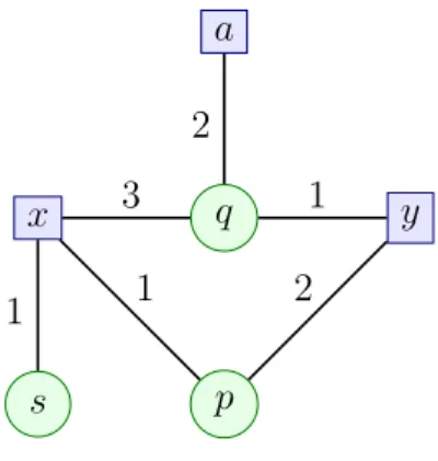
Consider the first-order formula F : ∃x∃y(p(x, y) ∧ q(y, a, x) ∧ s(x)); where a is a constant.
The formula F is an existentially closed conjunction of atoms, therefore a set of facts, which we can also denote by {p(x, y), q(y, a, x), s(x)}.
Sets of facts can also be seen as (hyper)graphs, which allows to apply several graph notions to them. Indeed, given a set of facts F , one can build a directed hypergraph whose set of vertices is in bijection with the set of terms of F , and whose set of hyperedges is in bijection with the set of atoms of F . Then each vertex is labelled by the corresponding term, and each edge by the predicate of the corresponding atom.
Example 1.2 (Graphical View of a Set of Facts)
Consider the set of facts F from Example 1.1. Figure 1.1 depicts its graphical representation, where hyperedges are represented via circle nodes.
Definition 1.20 (Conjunctive Query, Union of Conjunctive Queries) A conjunctive query (CQ) is a conjunction of atoms where all variables are either free (called answer variables) or existentially quantified.
A union of conjunctive queries (UCQ) is a disjunction of CQs with the same answer variables.
1.2. EXISTENTIAL RULE FRAMEWORK 13 x y a p q s 3 2 1 1 2 1
Figure 1.1: Graphical representation of the set of facts F from Example 1.1
If all variables of a conjunctive query Q are quantified (thus Q has the exact same form as a set of facts), we say that Q is a Boolean conjunctive query (BCQ). Throughout this thesis we only consider Boolean conjunctive queries that we simply call conjunctive queries.
A well-known fundamental result is that the logical consequence on existentially closed conjunctions of atoms (e.g., two sets of facts or Boolean conjunctive queries) amounts to the existence of a homomorphism as stated by the next theorem, which has been proven in several contexts (see, e.g., [AHV95] for a version in terms of classical CQ containment).
Let F1 and F2 be two sets of facts. There exists a homomorphism from F1
to F2 if and only if F2 |= F1.
Theorem 1.1 (Folklore)
Since one can compare two sets of facts with respect to logical consequence, it is natural to consider the core of a set of facts, which is a minimal equivalent subset. It should be pointed out that the definition of core we give here is restricted to finite sets of facts, which is enough for our needs. However, a more technical definition for infinite sets exists [Bod05].
Definition 1.21 (Core)
Given a finite set of facts F , a core of F is a minimal subset of F equivalent to F .
Example 1.3 (Core)
Consider the set of facts F = p(x, y) ∧ p(y, z) ∧ p(x, u) ∧ p(u, z). A core of F is p(x, y) ∧ p(y, z).
It is well-known that if F is a finite set of facts, then all its cores are isomorphic, for instance in Example 1.3, the set of facts p(x, u) ∧ p(u, z) is also a core of F .
Furthermore, given a set of facts F , one can define its “isomorphic model”, which has the same structure as F .
Definition 1.22 (Isomorphic Model)
Given a set of facts F built on the logical language L = (P, C), the isomorphic model of F denoted by M (F ) = (D, I) is defined as follows:
• D is in bijection with terms(F ) ∪ C (to simplify notations we consider that this bijection is the identity),
• for all c ∈ C, I(c) = c,
• for all p ∈ P, I(p) = {(t1, . . . , tk) | p(t1, . . . , tk) ∈ F }.
Finally, it is also well-known that the following properties are equivalent: given two sets of facts F1 and F2,
1. F1 |= F2,
2. there is a homomorphism from F2 to F1,
3. M (F1) is a model of F2.
An existential rule is a positive (and conjunctive) rule. Its special feature is that its head may introduce variables that do not occur in its body, and which are existentially quantified, hence the name “existential rule”. This allows to infer the existence of unknown individuals (possibly equal to (known) individuals appearing in the set of facts).
Definition 1.23 (Existential Rule)
An existential rule (or simply rule) on a logical language L is a closed formula of form ∀x1, . . . , ∀xb(B → ∃z1, . . . , zhH), where B and H are two finite conjunctions
of atoms on L, var(B) = {x1, . . . , xb} and var(H) \ var(B) = {z1, . . . , zk}.
The sets of atoms B and H are respectively called the body and the head of R. Variables occurring in var(B) ∩ var(H) are called the frontier variables of R and denoted by f r(R). Variables occurring in var(H) \ var(B) are called existential variables.
Since no ambiguity can arise, we omit the quantifiers in rules. Example 1.4 (Existential Rule)
Consider the rule R = ∀x∀y(p(x, y) → ∃z(p(y, z))). This rule will also be denoted by R = p(x, y) → p(y, z). Variable y is the only frontier variable of R and z is its only existential variable.
1.2. EXISTENTIAL RULE FRAMEWORK 15
Two other kinds of rules may be added to the framework: negative constraints, which are rules with an absurd head (B → ⊥), and equality rules which are rules whose head specifies the equality between two terms (B → t1 = t2). For details, see
[BLMS11, CGL09]. It should be pointed out that there is no additional complexity (or decidability) cost for considering negative constraints (except if only particular BCQ are considered). By contrast, equality rules are known for being hard to handle from both complexity and decidability points of view. In the following, we restrict our focus to knowledge bases without negative constraints nor equality rules. We are now ready to formally define a knowledge base.
Definition 1.24 (Knowledge Base)
A knowledge base is a pair K = (F , R) where F is a (finite) set of facts and R is a (finite) set of existential rules.
Note that, without loss of generality, we will always assume that sets of facts and all rules use disjoint sets of variables.
In the following, when we consider logical notions involving knowledge bases, sets of rules and/or facts, we implicitly consider the associated formula which is the conjunction of all involved formulae. In particular, (F , R) is seen as the conjunction of the formula associated with F and of all the rules from R.
A nice property of this setting is that given a knowledge base K = (F , R), there always exists a model of K that can be considered as a representative of all models of K, in the sense that is is sufficient to consider this model to check entailment from K. Such a model has the property of being “universal”.
Definition 1.25 (Universal Model)
Given a knowledge base K = (F , R), a universal model M of K is a model of K such that for all models M0 of K, there is a homomorphism from M to M0.
Note that not all knowledge bases have a finite universal model.
Now that we have defined all of our basics objects, we can reformulate the en-tailment problem more formally:
Given a knowledge base K = (F , R) and a Boolean conjunctive query Q, the conjunctive query entailment problem (CQ entailment) asks the following question: does K |= Q hold?
Problem 1.1 (Conjunctive Query Entailment)
It is well-known that this problem is undecidable (e.g., [BV81]), even under strong restrictions such as using a single rule or restricting the vocabulary (a single binary predicate, no constant, ...), see, for instance, [BLMS11].
However many restrictions on the set of rules are known to ensure decidability. Most of them can be classified in three families, which are associated with forward or backward chaining schemes [BLMS11]. The first one is that of Finite Expansion Sets (FES). It ensures that a finite universal model of the knowledge base exists. This property allows for some finite Forward Chaining, a process that “applies” rules until an answer to the query is found or nothing “useful” is produced. The second family is called Finite Unification Sets (FUS) and guarantees that some Backward Chaining method halts. This process uses the rules to “rewrite” the query which creates a UCQ, which is then checked against the initial set of facts. Finally, the last family is called Bounded Treewidth Set (BTS) [CGK08]. It ensures that the potentially infinite universal model of the knowledge base has a bounded treewidth. This class does not give an algorithm yet, but thanks to Courcelle’s theorem [Cou89], we know that entailment over BTS knowledge bases is decidable. Furthermore, an expressive subclass of BTS, namely Greedy BTS (GBTS) is provided with an algorithm [BMRT11, Tho13].
These classes will be precisely defined in Chapter 2.
1.2.1
Forward Chaining
Rules allow to infer new knowledge from an initial set of facts, giving rise to the notion of rule application. This notion is defined as usual in rule languages, i.e., the head of the rule is added to the set of facts according to a homomorphism from the body of the rule to the set of facts. The only specificity for existential rules is that existential variables in the rule head are replaced by fresh variables.
Definition 1.26 (Rule Applicability)
A rule R = B → H is applicable to a set of facts F if there exists a homomorphism π from B to F .
Definition 1.27 (Rule Application)
Given a set of facts F , a rule R = B → H and a homomorphism π from B to F , the result of the application of the rule R on F according to π is defined as
α(F , R, π) = F ∪ πsaf e(H)
where πsaf e if the extension of π to the existential variables of R, i.e.: for all variables
x occurring in H, πsaf e(x) = π(x) if x ∈ f r(R) and πsaf e(x) = z otherwise, where
z is a fresh variable (i.e., a variable that does not occur elsewhere).
Intuitively, πsaf e is a “safe” extension of π that maps all existential variables of
H to some distinct fresh variables, in order to avoid confusion with variables already occurring in F .
1.2. EXISTENTIAL RULE FRAMEWORK 17
Example 1.5 (Rule Application)
Let F = {c(a)} be a set of facts and R = c(x) → p(x, y) ∧ c(y) be an existen-tial rule.
Rule R is applicable to F since there exists the following homomorphism π = {x 7→ a}, and the application of R on F according to π produces the set of facts F1 = α(F , R, π) = c(a) ∧ p(a, y1) ∧ c(y1).
Then rule R is applicable to F1 thanks to the homomorphism π2 = {x 7→ y1},
which would produce p(y1, y2) ∧ c(y2) (and we could go on like this since each added
c-atom allows for a new application of R).
A sequence of rule applications is called a derivation and is defined as follows. Definition 1.28 (Derivation)
Given a set of facts F and a set of rules R, a derivation of F w.r.t. R (also called R-derivation) is a (potentially infinite) sequence D of triples of the form (Ri, πi, Fi)
such that D0 = (∅, ∅, F0 = F ), and ∀i > 0 in dom(D), Ri = (Bi, Hi) ∈ R, πi is a
homomorphism from Bi to Fi−1 and Fi = α(Fi−1, Ri, πi).
When D is of length k ∈ N, we say that it is a derivation from F to Fk.
Example 1.6 (Derivation)
Consider again the set of facts F = c(a), and the set of rules R composed of a single rule R = c(x) → p(x, y), c(y) from Example 1.5.
A derivation D of F with respect to R could be:
i Ri πi Fi 0 ∅ ∅ F 1 R {x 7→ a} F ∪ {p(a, y1), c(y1)}) . . . . k R {x 7→ yk−1} Fk−1∪ {p(yk−1, yk), c(yk)} . . . .
Note that in this example, only a single derivation (not using the same homo-morphism twice) is possible, but in general, this is not the case.
The next theorem states that derivations are a sound and complete way to “solve” the CQ entailment problem.
Let F be a set of facts, R be a set of rules, and Q be a Boolean conjunctive query; then, (F , R) |= Q if and only if there exists a (finite) R-derivation from F to Fk such that Fk|= Q.
Theorem 1.2 ([BLMS11])
Chapter 3 is devoted to the family of forward chaining algorithms and to rule classes for which some of these algorithms always halt.
1.2.2
Backward Chaining
In contrast with forward chaining, backward chaining mecanisms start from the query. In Prolog and other logic programming languages, facts are ground atoms (which possibly involve functional symbols) and are seen as rules with an empty body. The aim is then to “erase” the query by iteratively rewriting it with the rules. In knowledge representation, we clearly distinguish between rules and facts, hence we decompose the backward chaining into two processes: rewriting the query using the rules, and mapping a rewritten query to the set of facts (by homomorphism). The OBDA approach goes one step further by completing the rewriting process before trying to map the obtained query (or set of queries) to the set of facts. The aim is to come back to a classical database query answering problem.
Differently from classical unifiers used in logic programming which unify an atom from the query with the head atom, piece-unifiers do not consider a single atom of the query but a subset of the query. This allows to correctly process existential variables as illustrated by the next example.
Example 1.7 (Classical Unifier)
Consider the rule R = person(x) → hasP arent(x, z) which says that every per-son has a parent, and the set of facts F = perper-son(Bob) ∧ painter(M ax). As-sume one asks if someone has a parent who is a painter with the following query Q = ∃u, v(hasP arent(u, v) ∧ painter(v)). With a classical (most general) unifier of Q with the head of R, for instance {x 7→ u, z 7→ v}, we obtain the direct rewriting Q1 = ∃u, v(person(u) ∧ painter(v)) (in which the connection between u and v has
been lost). We then have that F |= Q1 while (F , R) 6|= Q. Hence, this rewriting is
unsound. Here the “piece condition” from the following definition of a piece-unifier has been violated.
Piece-unifiers can be seen as generalised unifiers, in the sense that they unify two sets of atoms. Moreoever they process existential variables in a special way.
The following definition of a piece-unifier considers the partition on terms induced by a (generalised) unifier: the terms unified together are in the same class of the partition. Partitions have nice properties that are convenient in proofs.
Definition 1.29 (Piece-unifier)
Given a rule R = (B, H) and a set of atoms Q, a piece-unifier of Q with H is a triple µ = (Q0, H0, Pµ) where Q0 ⊆ Q, H0 ⊆ H and Pµ is a partition of terms of
Q0∪ H0 such that:
(i) Admissibility: there is at most one single constant or existential variable from H0 in each class of Pµ, and if a class contains an existential variable, it
cannot contain a frontier variable from R (hence, the other terms in the class are from Q0);
(ii) Unifiability: σµ(Q0) = σµ(H0), where σµ is a substitution associated with the
1.2. EXISTENTIAL RULE FRAMEWORK 19
(iii) Piece condition: if there is an existential variable z occurring in H0 then no atom from Q \ Q0 may contain a variable x occurring in the same class as z. Definition 1.30 (Substitution Associated with a Partition)
Given an admissible partition of a set of terms Pµ, a substitution associated with Pµ
is obtained as follows: for each class C ∈ Pµ, choose a term tC ∈ C (if C contains
a constant, then tC must be that constant); then σµ = S C∈P
{t 7→ tC | ∀t ∈ C}. The
terms tC are said to be preserved by the substitution.
Note that when a class contains only variables, one can choose to give priority to variables occurring in the query or in the rule.
Example 1.8 (Piece-unifier)
Consider the rule R = p(x, y) → s(x, z) and the conjunctive query Q = s(a, u) ∧ s(v, u) ∧ r(v), where a is a constant. There is the following piece-unifier of Q with H:
{Q0 = {s(a, u), s(v, u)}, H0 = {s(x, z)}, Pµ = {{a, v, x}, {u, z}}}
Indeed, no class of Pµ contains more than one existential variable from H0 or
con-stant, and the class that contains an existential variable does not contain any frontier variable, thus admissibility is satisfied. One can choose for instance the substitution σµ = {v 7→ a, x 7→ a, u 7→ z}. We then check that σµ(Q0) = σµ(H0). Finally all
atoms of Q using variable u (which is unified with the existential variable z) belong to Q0, hence the piece condition is satisfied.
Note that no smaller piece-unifier of Q with H exists since u is necessarily unified with z, hence the piece condition requires that both atoms of Q are part of Q0.
Given this extended notion of unifier, we can now define a direct query rewriting as follows.
Definition 1.31 (Direct Query Rewriting)
Given a rule R = (B, H), a conjunctive query Q, a piece-unifier µ = (Q0, H0, Pµ) of
Q with H and a substitution σµ associated with Pµ, the direct query rewriting of Q
according to µ is the following CQ: β(Q, R, µ) = σµ(Q \ Q0) ∪ σµ(B).
Note that in the above definition any substitution associated with µ can be used, as they all give isomorphic results.
Example 1.9 (Direct Rewriting)
Consider the rule R, the query Q and the piece-unifier µ from Example 1.8. The direct rewriting of Q according to µ is: β(Q, R, µ) = r(a) ∧ p(a, y).
Definition 1.32 (Rewriting Sequence)
Given a CQ Q, and a set of rules R, a rewriting sequence of Q w.r.t. R (also called an R-rewriting sequence) is a (potentially infinite) sequence S of triples (Ri, µi, Qi)
such that S0 = (∅, ∅, Q) and ∀i > 0, Ri = (Bi, Hi) ∈ R, µi is a piece-unifier of Qi−1
with Hi and Qi = β(Qi−1, Ri, µi).
When S is of length k ∈ N, we say that it is a rewriting sequence from Q to Qk.
Similarily to derivations, rewriting sequences are a sound and complete way to “solve” the CQ entailment problem as stated by the next theorem.
Let F be a set of facts, R be a set of rules and Q be a Boolean conjunctive query; then, (F , R) |= Q if and only if there exists a rewriting sequence from Q to Qk such that F |= Qk.
Theorem 1.3 ([BLMS11])
This notion gives naturally rise to an algorithm that reads: let Q = {Q}, for all queries Qi ∈ Q, rewrite Qi according to some unifier, then add the result to Q if it
is not equivalent to another query. If at some point no new query is added, end the process and evaluate the union of conjunctive queries on the knowledge base.
While both of these scheme families seem quite different, they are actually strongly related in the sense that given a knowledge base K = (F , R) and a Boolean conjunctive query Q, if there exists a derivation of F w.r.t. R of length k such that Fk entails Q, then there exists a rewriting sequence of at most length k leading to
a query Q0 entailed by F ; and if there exists a rewriting sequence of length k such that F entails Qk, then there exists a derivation of same length leading to a set of
facts Fk such that Fk entails Q, as stated by the next theorem.
Note that the derivation may be longer than the rewriting sequence, since in the former one can add rule applications that are useless to answer Q.
Let F be a set of facts, R be a set of rules and Q be a conjunctive query. If there exists a derivation from F to Fksuch that Fk|= Q, then there exists
k0 ≤ k and a rewriting sequence from Q to Qk0 such that F |= Qk0.
Furthermore, if there exists a rewriting sequence from Q to Qk such that
F |= Qk, then there exists a derivation from F to Fk such that Fk |= Q.
1.3. SOME USEFUL TRANSLATIONS 21
1.3
Some Useful Translations
In this section we define several transformations of sets of rules (with one of them also involving a translation of the set of facts), mostly used to simplify the shape of the rules we need to consider.
The first translation is used to convert rules into single-piece headed rules. We define first the “piece graph” of a rule that allows us to easily define the notion of piece.
Definition 1.33 (Piece Graph)
Given a rule R = (B, H) its piece graph is defined as the undirected graph whose set of vertices is the set of atoms occurring in H, and where there is an edge between two vertices corresponding to atoms h1 and h2 in H if there is an existential variable
z such that z ∈ var(h1) and z ∈ var(h2).
Definition 1.34 (Rule Piece, Single-piece Headed Rule)
Given a rule R = (B, H), a rule piece of R is the set of atoms corresponding to a connected component of the piece graph of R.
A rule R is a single-piece headed rule if H is a single rule piece of R.
Intuitively, a rule piece corresponds to the minimal unit of information contained in a rule head. Indeed, any rule can be decomposed into an equivalent set of rules with the same body and a head restricted to a single rule piece as performed by the following translation.
Definition 1.35 (Single-piece Translation)
Given a set of rules R, its single-piece translation sp(R) is defined as follows. For each rule R = (B, H) ∈ R, for each rule piece Hi of R, add in sp(R) the rule
B → Hi.
This transformation is without loss of generality, hence, we can always assume that all rules we consider are single-piece.
Given a set of rules R, R and sp(R) are logically equivalent. Proposition 1.1
Example 1.10 (Single-piece Translation)
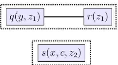
Consider the following rule (where c is a constant and every other term a variable): R = p(x, y, c) → q(y, z1) ∧ r(z1) ∧ s(x, c, z2).
The piece graph of R is depicted on Figure 1.2.
q(y, z1) r(z1)
s(x, c, z2)
Figure 1.2: Piece Graph of rule R from Example 1.10 • R1 = p(x, y, c) → q(y, z1) ∧ r(z1)
• R2 = p(x, y, c) → s(x, c, z2)
The next translation further simplifies the shape of rules we consider. Definition 1.36 (Atomic-headed Translation)
Given a set of rules R its atomic-headed translation ah(R) is defined as follows. For each rule R = (B, H) ∈ sp(R) where |H| > 1, perform the following:
1. create a new predicate rR of arity |var(H)|,
2. add to ah(R) the rule B → rR(~t) where ~t is the set of variables occurring in
H,
3. for each atom hi ∈ H, add the rule rR(~t) → hi to ah(R).
This translation creates new predicates with arity depending on the size of a rule head, and thus is not suitable in a context where we consider that the arity is bounded. However, if the arity is not assumed to be bounded, it will prove useful to be able to simplify rule heads into single atoms.
Example 1.11 (Atomic-headed Translation)
Consider again the rule R from Example 1.10, and its single-piece translation sp(R) = {R1, R2}. Its atomic-headed translation is the following set of rules:
• R1,a= p(x, y, c) → rR1(y, z1)
• R1,b1 = rR1(y, z1) → q(y, z1)
• R1,b2 = rR1(y, z1) → r(z1)
• R2 = p(x, y, c) → s(x, c, z2)
Note that this translation could be defined on any set of rules R without first decomposing it into sp(R), however it would potentially create predicates with an arity larger than needed.
1.3. SOME USEFUL TRANSLATIONS 23
Let R be a set of rules. For any CQ Q and knowledge base (F , R) on a logical language L, (F , R) |= Q iff (F , ah(R)) |= Q.
Proposition 1.2
The last translation we consider is used to get rid of constants occurring in rules. As for the atomic-headed translation, this cannot be used without loss of generality in the case where the arity is bounded. Furthermore, this translation not only modifies the rules, but also the set of facts. The idea is to totally order the constants, say from c1 to cn, and increase the arity of each predicate by creating
a placeholder for each constant. Then rules are translated in such a way that p(. . . , c, . . . ) where c is the ith constant becomes p0(. . . , x
i, . . . , x1, . . . , xn), where xi
stands for the ith constant. Hence the occurrence of the ith constant in an atom is replaced by the double occurrence of the variable xi. Facts are translated by adding
c1, . . . , cn at the end of each atom.
Definition 1.37 (No-constant Translation)
Given a knowledge base K = (F , R), its no-constant translation nc(K) is defined as follows. For each predicate p of arity k, create a new predicate p0 with arity k + |cst(K)|, where cst(K) = {c1, . . . , cn} is the set of all constants occurring either
in F or in some rule R ∈ R.
Then for each atom α = p(t1, . . . , tk) in some rule R ∈ R, replace α by an atom
p0(t01, . . . , t0k, . . . , t0k+n) where (all xj being distinct fresh variables):
t0i = ti if i ≤ k and ti is a variable, xj if i ≤ k and ti = cj, xj if i = k + j.
Now for each atom α = p(t1, . . . , tk) in F , replace α by an atom p0(t1, . . . , tk, c1, . . . , cn).
Finally, for each predicate p create the rule p0(y1, . . . , yk, x1, . . . , xn) → p(y1, . . . , yk),
where all variables are distinct.
Example 1.12 (No-constant Translation)
Consider again rule R = p(x, y, c) → q(y, z1) ∧ r(z1) ∧ s(x, c, z2) from Example
1.10, and let F = p(b, b, b) ∧ p(b, b, c) be a set of facts, where b is a constant.
The no-constant translation of K = (F , {R}) is obtained as follows. The set of constants is {b, c}, hence n = 2. First we create four new predicates p0, q0, r0 and s0 of arity 5, 4, 3 and 5 respectively. Now we update rule R into:
R0 = p0(x, y, x2, x1, x2) → q0(y, z1, x1, x2) ∧ r0(z1, x1, x2) ∧ s0(x, x2, z2, x1, x2)
Then the set of facts becomes F0 = p(b, b, b, b, c) ∧ p(b, b, c, b, c). Finally we add the following four rules (one for each predicate):
• Rp = p0(y1, y2, y3, x1, x2) → p(y1, y2, y3),
• Rq = q0(y1, y2, x1, x2) → q(y1, y2),
• Rr = r0(y1, x1, x2) → r(y1),
• Rs = s0(y1, y2, y3, x1, x2) → s(y1, y2, y3).
These four rules allow to transfer facts from the new vocabulary to the original one.
Let R be a set of rules. For any CQ Q and knowledge base (F , R) on a logical language L, (F , R) |= Q iff nc(F , R) |= Q.
Proposition 1.3
In particular, in Section 4.2, we will make the assumption that all rules are single-headed rules and contain no constant, and this will allow for simpler decidability proofs.
Furthermore, note that both the atomic-headed and the no-constant translations only preserve answers on the original vocabulary. Indeed, new predicates are created, and thus, queries that would involve these new predicates may have a positive answer in the translation but not in the original knowledge base.
Conclusion
The next chapters will rely on the fundamental notions we have introduced here: • Chapter 2: this chapter is devoted to rule classes for which the CQ entailment
problem is decidable. Derivations and rewriting sequences are the fundamental mechanisms that underly these classes.
• Chapter 3: several forward chaining (or “chase”) mechanisms can be based on the derivation notion, and after recalling most of them, we study the var-ious acyclicity conditions that ensure the finiteness of some forward chaining variant.
• Chapter 4: we study the compatibility of transitivity rules with other known decidable classes of rules. The algorithm we develop for the case of linear rules is based on backward chaining techniques.
Chapter 2
Landscape of Decidable Classes of
Rules
Contents
2.1 Abstract Rule Classes . . . 25 2.2 Finite Expansion Set . . . 28 2.3 Bounded Treewidth Set . . . 33 2.4 Finite Unification Set . . . 37 2.5 Description Logics . . . 43 2.6 Kiabora . . . 46 In this chapter we review various decidability and complexity results from the literature for the CQ entailment problem. More specifically, we recall the main classes of rules C such that entailment over knowledge bases where the set of rules belongs to C is decidable. For brevity reasons, we often refer to them as “decidable classes of rules”. We end this chapter by pointing out the relationships between description logics and the existential rule framework.
2.1
Abstract Rule Classes
First, we recall three abstract rule classes, “abstract” in the sense that we cannot decide in general whether a set of rules belongs to one of them [BLMS11]. These classes ensure a specific behaviour of either some forward or some backward chaining algorithm.
Definition 2.1 (Finite Expansion Set (FES) [BLMS11])
Given a set of rules R, we say that R satisfies the Finite Expansion Set (FES) property if for any set of facts F , there exists some k ∈ N such that for any query Q, there exists a (finite) derivation from F to Fk such that Fk |= Q if and only if
(F , R) |= Q.
The Finite Expansion Set property ensures that for any set of facts F , the knowledge base (F , R) has a finite universal model. Hence a forward chaining algorithm that applies rules in a “breadth-first” manner (also known as the “chase”), and after each rule application (or after each breadth-first step) considers the core of the obtained set of facts halts on any knowledge base built with a set of rules satisfying the FES property. Then, the isomorphic model of the saturated set is finite. More details on the different kinds of chase and their properties are given in Section 3.1.
Example 2.1 (Non-FES)
The set of rules composed of the single rule R = q(x) → p(x, y) ∧ q(y) is not FES. Indeed, consider the set of facts q(a). Then one can apply rule R according to homomorphism π1 = {x 7→ a} and obtain F1 = q(a) ∧ p(a, y0) ∧ q(y0). A core of F1 if
F1 itself. The rule R can be applied again, this time using the homomorphism π2 =
{x 7→ y0} and the resulting set of facts is F2 = q(a)∧p(a, y0)∧q(y0)∧p(y0, y1)∧q(y1).
One can see that this rule can be applied again, and this process will never halt. The second abstract property relies on query rewriting. A set of rewritings Q of a query Q with a set of rules R is said to be sound and complete if for any set of facts F , it holds that (F , R) |= Q if and only if there is Qi ∈ Q such that F |= Qi
(the direction ⇒ expresses the soundness while the direction ⇐ the completeness). When Q is finite, it can be seen as a union of conjunctive queries. Then the previous condition can be recast as: (F , R) |= Q iff F |= Q.
Definition 2.2 (Finite Unification Set [BLMS11])
Given a set of rules R, we say that R satisfies the Finite Unification Set (FUS) property if for any query Q, there is a finite sound and complete set of rewritings of Q with R.
This set is clearly computed independently from any set of facts. Note that the FUS property can also be expressed as follows: a set of rules R is FUS if and only if for any conjunctive query Q, there is some k ∈ N such that the set of all (sound) rewritings of Q with R that can be obtained by a rewriting sequence of length less than or equal to k is complete. In other words, Q is “UCQ-rewritable”.
This property ensures that given a set of rules R that satisfies it, any conjunctive query Q can be rewritten into a (finite) union of conjunctive queries Q such that for any set of facts F , (F , R) entails Q if and only if there is a rewriting Q0 ∈ Q, such that F entails Q0. Note that a FUS set of rules may have an infinite sound set of rewritings. However this set always has a finite complete subset obtained by ignoring redundant queries, i.e., queries Q2 that are contained in another query Q1
(which can be checked by exhibiting a homomorphism from Q1 to Q2). In other
words, for any query Q there exists some k ∈ N such that the set Q of all sound rewritings of Q obtained by a sequence of length less than or equal to k is complete. Hence, if a knowledge-base is built on a finite unification set of rules, then a query
2.1. ABSTRACT RULE CLASSES 27
rewriting algorithm that would after each rewriting only keeps the queries that are not contained in another one halts, see [KLMT15] for such an algorithm.
It has been shown in [LMU16] that FUS is equivalent to the Bounded Derivation Depth Property (BDDP) [CGL09] defined as follows: for any query Q, there exists some k ∈ N such that for any set of facts F, (F, R) |= Q if and only if there exists a (finite) derivation from F to Fk such that Fk |= Q. This allows to relate the notions
of derivations and rewriting sequences for FUS rules: for any query Q there exists some k ∈ N such that for any set of facts F, (F, R) |= Q if and only if there is a (finite) derivation from F to Fk such that Fk |= Q if and only if there is a (finite)
rewriting sequence from Q to Qk such that F |= Qk.
Furthermore, in [GKK+14], it is shown that the BDDP is equivalent to First-order Rewritability, i.e., to the existence of a first-First-order formula ϕ(Q) such that (F , R) |= Q if and only if F |= ϕ(Q). While a UCQ rewriting is already a spe-cific kind of first-order rewriting, there may exist a first-order rewriting exponen-tially smaller than all UCQ rewritings. In turn, every first-order rewriting can be translated into an equivalent UCQ-rewriting (which, however, can be exponentially larger). Such rewriting can thus be useful from a practical point of view, since most databases query languages (such as SQL) allows for first-order querying.
Example 2.2 (Non-FUS)
The following set of rules {p(x, y) ∧ p(y, z) → p(x, z)} is not FUS. For instance the query Q = p(a, b) does not admit a finite sound and complete set of rewrit-ings. Indeed, any sound and complete set of rewritings of Q contains p(a, b) and the queries p(a, y0) ∧ p(y0, y1) ∧ . . . p(yk, b) for all k ∈ N. Note that all these queries are
pairwise incomparable with respect to containment.
The last abstract property relies on the notion of treewidth of a set of facts. To compute such treewidth, we use the primal graph of a set of facts F , which is the undirected graph defined as follows: the set of vertices is the set of terms occurring in F and there is an edge between two vertices u and v if there is an atom α ∈ F such that the terms corresponding to u and v occur both in α. Then the treewidth of F is the treewidth of the primal graph of F .
Definition 2.3 (Bounded Treewidth Set (BTS) [CGK08, BLMS11]) A set of rules R is a bounded treewidth set (BTS) if for any set of facts F , there exists b ∈ N such that for any derivation from F to Fk the core of Fk has treewidth
at most b.
This property can also be expressed in terms of models: a set of rules R is BTS if and only if there exists a (potentially infinite) universal model of the knowledge base whose treewidth is bounded.
Example 2.3 (Non-BTS)
• R1 = q(x) → p(x, y) ∧ q(y)
• R2 = p(x, y) ∧ p(y, z) → p(x, z)
The set of rules R is not BTS. Indeed, the first rule creates an infinite path, while the second computes the transitive closure of this path. Consider for instance the set of facts restricted to a single atom q(a). For any k ∈ N, the set of facts obtained from q(a) by all derivations of length at most k “encodes” a clique of size k (more precisely, its primal graph contains such a clique), hence its treewidth is at least k. Furthermore, it is not possible to suppress this clique by considering the core of the set of facts (actually, under reasonable assumptions on the forward chaining mechanism, the generated set of facts is itself a core). It follows that any universal model of this knowledge base has unbounded treewidth.
Obviously, any FES set of rules is also a BTS set of rules, indeed it suffices to consider the number of terms occurring in a finite universal model as the bound on its treewidth. The decidability relies on Courcelle’s Theorem [Cou89], which states that for any logical fragment in which the existence of a model implies the existence of a bounded treewidth model, then the satisfiability of a property that can be expressed in monadic second-order logic is decidable. However this does not provide explicitly an algorithm to answer the entailment problem. Though, there exists an expressive subclass of BTS called Greedy Bounded Treewidth Set (GBTS), for which we do not give a formal definition. Since we will not study it in this thesis, see [BMRT11, RT14, Tho13] for more details. Intuitively, this class ensures that one can build a bounded width tree decomposition of the saturated set of facts greedily, and furthermore compute a finite structure that encodes this tree decomposition. We do not know yet if this class is concrete or abstract, i.e., whether the associated recognition problem is decidable; though, this class is very interesting since on the one hand, a practical algorithm is provided, and on the other hand, to our knowledge, it includes all but one concrete known rule classes belonging to BTS but not to FES.
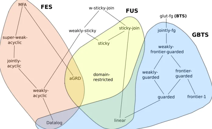
For each of these abstract rule classes, various concrete rule subclasses have been exhibited. In the following, we detail the main ones, and Figure 2.1 pictures the relations between them: an upwards edge going from a rule class C to a rule class C0 means that any set of rules in class C is also in class C0.
2.2
Finite Expansion Set
Regarding FES rule classes, most of them can be classified in two different subfam-ilies (Section 3.2 is dedicated to them). The first family relies on how existential variables interact with each others, while the second one on how rules are triggered.
2.2. FINITE EXPANSION SET 29 acyclic jointly-acyclic weakly-acyclic Datalog aGRD sticky weakly-sticky w-sticky-join sticky-join linear guarded frontier-1 frontier-guarded weakly-guarded weakly-frontier-guarded jointly-fg glut-fg MFA domain-restricted FES FUS GBTS (BTS)
Figure 2.1: Relations between known decidable rule classes
In the first family, the simplest of all classes is that of range-restricted, or Datalog rules (as it corresponds exactly to the rules in Datalog queries). In these rules, no existential variable appears.
Definition 2.4 (Range-restricted (rr) [AHV95])
A set of rules R is range-restricted if no existential variable occurs in a rule from R.
This rule class, while it seems really simple, allows to already express various interesting ontological properties, such that symmetry, transitivity, ...
Example 2.4 (Range-restricted)
Consider the set of rules R composed of the following rules: • p(x, y) ∧ p(y, z) → p(x, z)
• p(x, y) → p(y, x)
These rules assert that p is a transitive and symmetric binary relation. The set of rules R is range-restricted.
This class has been first extended to allow for existential variables while limit-ing the way they propagate durlimit-ing the forward chainlimit-ing, in order to avoid infinite creation of new variables. This constraint relies on a graph of predicate positions as defined below, where to ease the reading we denote by (p, i) the ith position in
predicate p.
Definition 2.5 (Predicate Position Graph)
Given a set of rules R, its predicate position graph, denoted by P P G(R) is the directed labelled graph whose set of vertices is the set of predicate positions of R. Then for each rule R ∈ R and each frontier variable x in B occurring in some po-sition (p, i), edges with origin (p, i) are built as follows: there is an edge from (p, i) to each position (q, j) in H where x occurs, and there is a special edge from (p, i) to each position (q, j) in H where some existential variable y appears.
Then we say that the rank of a predicate position (p, i) is infinite in a set of rules R if (p, i) belongs to a cycle going through a special edge in P P G(R), and is finite otherwise.
The intuition behind this graph is that edges translate how terms can move from a position to another. Furthermore, its special edges mark the generation of existential variables, and if a cycle contains a special edge then an existential variable may lead to generate a new existential variable in the same position, hence may lead to infinitely many new existential variables.
Definition 2.6 (Weak-acyclicity (wa) [FKMP05])
A set of rules R is weakly-acyclic if its predicate position graph does not contain any cycle going through a predicate position in which an existential variable occurs, i.e., if all predicate positions have finite rank.
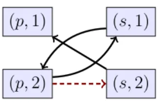
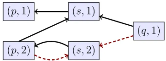
Example 2.5 (Weak-acyclicity)
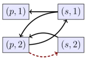
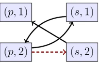
Consider rules R1 = p(x, y) → s(y, z) and R2 = s(x, y) → p(y, x). The set of
rules {R1, R2} is weakly-acyclic as its predicate position graph does not contain any
“special cycle” (i.e., a cycle going through a special edge), hence, all positions are of finite rank as can be seen on Figure 2.2.
(p, 1)
(p, 2)
(s, 1)
(s, 2)