Copyright1998 by the Genetics Society of America
A Rank-Based Nonparametric Method for Mapping Quantitative
Trait Loci in Outbred Half-Sib Pedigrees: Application to
Milk Production in a Granddaughter Design
Wouter Coppieters,* Alexandre Kvasz,* Fre´de´ric Farnir,* Juan-Jose Arranz,* Bernard Grisart,*
Margaret Mackinnon
†and Michel Georges*
*Department of Genetics, Faculty of Veterinary Medicine, University of Lie`ge, 4000 Lie`ge, Belgium and†Institute of Cell,
Animal and Population Biology, University of Edinburgh, Edinburgh, EH9 3JT, United Kingdom
Manuscript received November 6, 1997 Accepted for publication March 30, 1998
ABSTRACT
We describe the development of a multipoint nonparametric quantitative trait loci mapping method based on the Wilcoxon rank-sum test applicable to outbred half-sib pedigrees. The method has been evaluated on a simulated dataset and its efficiency compared with interval mapping by using regression. It was shown that the rank-based approach is slightly inferior to regression when the residual variance is homoscedastic normal; however, in three out of four other scenarios envisaged, i.e., residual variance heteroscedastic normal, homoscedastic skewed, and homoscedastic positively kurtosed, the latter outper-forms the former one. Both methods were applied to a real data set analyzing the effect of bovine chromosome 6 on milk yield and composition by using a 125-cM map comprising 15 microsatellites and a granddaughter design counting 1158 Holstein-Friesian sires.
R
ECENT developments in DNA marker technology, populations, generated as part of the appliedprogeny-test breeding design. such as the discovery of microsatellites (Weber
and May 1989), random amplified polymorphic DNA A number of mapping methods have been applied to
such half-sib designs, including single-marker regres-(RAPDs; Williams et al. 1990), and amplified fragment
length polymorphism (AFLPs; Vos et al. 1995) as abun- sion (e.g., Cowan et al. 1990), interval mapping using
regression (e.g., Knott et al. 1996), and maximum like-dant sources of well-dispersed genetic markers, have
boosted the construction of marker maps across a broad lihood methods (e.g., Georges et al. 1995). All these
methods share a common assumption, namely the resid-taxonomic range. Not only are such maps now available
for human and model organisms such as mouse and ual normal distribution and homoscedasiticity of the
analyzed phenotypes or transformations thereof. These rat but for a number of agriculturally important animal
and plant species as well. approaches therefore are not suitable for phenotypes
that are known not to satisfy this normality assumption. These maps increasingly are applied to locate genes
underlying inheritable phenotypes of interest. Several Moreover, deviations from normality for traits that
gen-erally are assumed to be quasi-normally distributed are of the most relevant phenotypes are continuously
dis-tributed quantitative traits involving multiple polygenes likely to affect the power and robustness of these conven-tional approaches.
or quantitative trait loci (QTL), as well as nongenetic
effects. Experimental back- and intercrosses are often Recently, Kruglyak and Lander (1995a) described
a nonparametric QTL interval mapping approach based the preferred design to map QTL. However, in a
num-ber of agriculturally important species (notably cattle on the Wilcoxon rank-sum test applicable in
experimen-tal crosses. This method provided a robust alternative and pine trees), reproductive cycles and breeding
de-to conventional approaches, applicable de-to normally dis-signs have led to the generation of extensive half-sib
tributed traits with minimal loss of power and extending pedigrees that are readily available for QTL mapping.
the scope of QTL mapping to a variety of traits not A well-documented example of this is the so-called
normally distributed, such as counts generated by a Pois-granddaughter design to map genes underlying milk
son process, truncated data, probabilities, and qualita-production in commercial cattle populations (Weller
tive data.
et al. 1990). This design takes advantage of the numerous
In this article, we describe the adaptation of this paternal half-brother pedigrees that exist in dairy cattle
method to half-sib pedigrees in outbred populations and apply it to milk production in a granddaughter design. A computer program to implement this ap-Corresponding author: Michel Georges, Department of Genetics,
Fac-proach has been developed and is available from the
ulty of Veterinary Medicine, University of Lie`ge (B43), 20 Bd de
Colonster, 4000 Lie`ge, Belgium. E-mail: [email protected] authors upon request.
MATERIALS AND METHODS population frequency of the obliged maternal marker allele of marker m, given the paternal gamete k.
A QTL interval mapping procedure based on the Wilcoxon All marker phases are a priori considered to be equally likely; rank-sum test—general principles:To measure the evidence i.e., linkage equilibrium is assumed to be reached between all in favor of a QTL at a given map position, Kruglyak and markers. The marker phase maximizing the likelihood of the Lander(1995a) define the following statistic (illustrated for pedigree data is considered the true one and is selected for
an (A3 B) 3 A backcross), further analysis.
As pointed out by Kruglyak and Lander (1995a),
ZW(s)5 YW(s)/√kYW(s)2l, (1)
kYW(s)2l 5
1
n32 n
3
2
k[1 2 2·P[gi,A(s)|gi,L,gi,R]]2l. (4)
where
YW(s)5
o
n i51
[n1 1 2 2 · rank (i)] Whilek[1 2 2·P[gi,A(s)|gi,L,gi,R]]2l or the expected value of
[12 2·P[gi,A(s)|gi,L,gi,R]]2 over all possible genotypes is
com-puted easily for experimental crosses, its calculation is more ·[P[gi,A(s)|gi,L,gi,R]2 P[gi,B(s)|gi,L,gi,R]], (2)
cumbersome in outbred designs as it will depend on marker in which n is the number of progeny; rank(i) is the rank by allele frequencies and genotype of the founder sire. The value phenotype of progeny i; P[gi,A(s)|gi,L,gi,R] is the probability that ofk[1 2 2·P[gi,A(s)|gi,L,gi,R]]2l is therefore calculated for each
progeny i has genotype AA at map position (s) given its half-sib pedigree by simulating all possible offspring and calcu-genotype at the left (gi,L) and right (gi,R) flanking markers; lating a frequency weighted mean of [12 2·P[gi,A(s)|gi,L,gi,R]]2.
P[gi,AB(s)|gi,L,gi,R] is the probability that progeny i has genotype Across family analysis:In practice, the available pedigree
AB at map position (s) given its genotype at the left (gi,L) and material is composed most often not of one half-sib pedigree
right (gi,R) flanking markers; and but of a series of such half-sibships, such as in the
grand-daughter design (Weller et al. 1990). In outbred populations,
√kYW(s)2l however, the different sibships cannot be assumed to segregate
for the same QTL or even QTL alleles; i.e., one cannot assume is the standard deviation of YW(s), expected under the null
locus and allelic homogeneity across families. hypothesis of no QTL over all possible sets of genotypes.
Rather than analyze the pedigrees separately, however, and Under the null hypothesis of no QTL, ZWis shown to behave
reduce power by multiple testing, the individual ZW(s) scores
asymptotically as a standard normal variable that reduces to
were squared and summed over all k families yielding a x2
a Wilcoxon rank-sum test at the marker positions.
statistic with k degrees of freedom: Adaptation to outbred half-sib designs:The method
devel-oped by Kruglyak and Lander (1995a) for experimental
o
kj51
[ZW(s)j]25 x2k. (5)
crosses was adapted to outbred half-sib designs, e.g., a founder sire mated to several dams to produce a large paternal
half-Interval mapping by regression: The rank-sum-based ap-sibship. The approach relies on the same ZW(s) statistic.
How-proach (hereafter referred to as method RS) was compared ever, P[gi,A(s)|gi,L,gi,R] (Equation 2) is now defined as the
proba-with interval mapping by using regression (hereafter referred bility that progeny i has inherited QTL allele A from the
to as method MR for multipoint regression; Knott et al. 1996). founder sire—assumed to be heterozygous AB at the QTL—at
For each half-sib family, j, phenotypes were regressed on map position (s) given its genotype at the left (gi,L) and right
P[gi,A(s)|gi,L,gi,R], calculated as described above, yielding
least-(gi,R) flanking markers. Only markers for which the founder
squares estimators of the y intercept,b0j, and the slope,b1j,
sire is heterozygous are considered when computing P[gi,A(s)|
the latter being an estimator of the QTL allele substitution
gi,L,gi,R]. Moreover, while the nearest flanking markers contain
effect in the corresponding family, j. The ratio all information needed to compute P[gi,A(s)|gi,L,gi,R] in a given
interval when dealing with experimental crosses, information
from more distant markers is considered in the outbred half- (Rkj51SSRj/k)
(Rk
j51SSEj/(n2 2k))
sib situation, when closer markers are not fully informative.
This occurs in the case of missing genotypes or when the was used to measure the evidence in favor of a segregating offspring has the same marker genotype as the sire, and the QTL at chromosome position (s). n is the total number of dam is either not genotyped or has the same heterozygous observations, k is the number of half-sib families, and SSR
j
genotype as well. In the former case, part of the information (sum of squares regression) measures the variability in the can be recovered by considering marker allele frequencies in
phenotype attributed to the segregation of a hypothetical QTL the population.
at position (s) in family j, and SSEj(sum of squares error)
Calculation of P[gi,A(s)|gi,L,gi,R] requires knowledge of the measures the residual or unexplained phenotypic variability
sire’s marker linkage phase. In the absence of grandparental
in family j. This ratio can be shown to be distributed as an marker information, the most likely linkage phase is first
esti-F-statistic under the null hypothesis of no QTL at the
corre-mated from the marker genotypes of the offspring. This is
sponding chromosome position. accomplished by calculating the likelihood of the pedigree
Significance thresholds:For both the RS and MR methods, data under the 2x/2 possible phases (assuming x informative
chromosome-wise significance thresholds were determined markers) as follows (Georges et al. 1995):
from the distribution of the test statistic over 10,000 permuta-tions (simulated data set) or 100,000 permutapermuta-tions (real data
Li5
p
n j513
o
2x k513
P(k|i)p
x m51AFMm
44
, (3) set) of the phenotypes (or ranks) as suggested by Churchilland Doerge (1995). Phenotypes were permutated within family. For each permutation, the highest value of the test where Li is the likelihood of the pedigree data for linkage
phase i;Pn
j51is the product over all n half-sibs; R2xk51is the sum statistic over the entire chromosome was retained to yield
“chromosome-wise” distributions of the test statistic under the over all possible sire’s gametes k; P(k|i) is the probability of
gamete k given Mendelian laws, phase i, and recombination null hypothesis. For the real data set, a Bonferonni correction was applied to the chromosome-wise significance level, consid-rates between adjacent markers,u1toux;Pxm51is the product
au-tosomes and that we analyzed the equivalent of three indepen- s2
R5p21 2pqr 1 q2s.
dent traits (Spelman et al. 1996) to obtain “experiment-wise”
Homoscedastic, skewed residual variance: Skewness was
simu-significance thresholds.
lated by assuming a residual effect distributed as a chi-squared Simulated data set: To test the efficacy of the proposed
distribution with n degrees of freedom, with variance s2 R5
method, we simulated the segregation of a QTL in a
grand-2n and mean n. Individual phenotypic values were generated
daughter design. The pedigree material was composed of two
as the mean of the genotypic class to which the individual paternal half-sib families of 100 sons, four families of 50 sons,
belongs (QQ5 a 2 n, Qq 5 0 2 n, or qq 5 2a 2 n) plus a and eight families of 25 sons, quite accurately reflecting a
value drawn from a chi-squared distribution with n degrees real data set. The 14 respective sires were considered to be
of freedom, obtained by summing n squared values drawn unrelated.
from a standard normal. A QTL was positioned in the center of the fourth interval
Homoscedastic, positive kurtosis: Excess of kurtosis was
simu-of a map comprising seven markers spaced 15
recombina-lated by assuming that the residual effect was distributed as tion units apart. Markers were assumed to be polyallic markers
a Student’s t -distribution with n degrees of freedom, with with frequencies randomly assigned from a uniform
dis-variances2
R5 n/(n 2 2) and mean 0. Individual phenotypic
tribution and rescaled to sum to unity, yielding a
heterozy-values were generated as the mean of the genotypic class to gosity of
which the individual belongs (QQ5 a, Qq 5 0, or qq 5 2a) plus a value drawn from a t -distribution with n degrees of
h5 1 2
#
1 0 ...#
1 0#
1 0 Rb i51p2i (Rb i51pi)2 ·dp1·dp2...dpb, freedom, i.e., Z/1
√x2 n/n2
.where piis the frequency of the ith allele randomly chosen
from the uniform distribution for the locus in question. The
Homoscedastic, negative kurtosis: Negative kurtosis was
simu-number of marker alleles was set at four, yielding an expected
lated by assuming that the residual effect was distributed as a heterozygosity of 67%, which is very comparable to what is
hemicircular distribution with mean 0 and variances2 R5 r2/
observed in reality with microsatellite markers in cattle
popula-4, where r is the radius of the hemicircle. Individual pheno-tions.
typic values were generated as the mean of the genotypic class The QTL was assumed to be biallelic with frequencies p5
to which the individual belongs (QQ 5 a, Qq 5 0, or qq 5 0.25 (Q) and q5 0.75 (q), respectively. Founder-sires therefore 2a) plus a value drawn from this hemicircular distribution. had an a priori probability 2pq5 0.375 to be heterozygous Qq
This was done by determining the value of t such that for the QTL. Following Falconer’s notation (Falconer and
MacKay1996) and assuming additively acting alleles, the aver- 2
pr2
#
t
0
√r22 x2dx5 s,
age phenotypic values of the QQ, Qq, and qq genotypic classes were set at1a, d 5 0, and 2a, respectively. Assuming
Hardy-Weinberg equilibrium, this yields an average effect of an allele where s is a random number between 0 and 1.
substitution,a 5 a, and a variance attributable to the segrega- Figure 1 illustrates the expected phenotypic distributions
tion of the QTL: of offspring from heterozygous founder-sires, Qq, for the five
examined models. Offspring are sorted in two genotypic s2
QTL5 2pqa2. classes depending on the QTL allele transmitted by the sire
(Q or q). Each class therefore comprises two subpopulations:
The value of a was determined such that QQ (25%) and Qq (75%) for the Q class and Qq (25%) and
qq (75%) for the q class.
At least 200 datasets (ranging from 200 to 866) were
simu-h25 s 2 QTL s2 P 5 s2QTL s2 QTL1 a2R 5 2pqa2 2pqa21 a2
R lated under each of the five models of residual variation and
analyzed with the RS and MR methods. Permutations were
reached a constant percentage, or used to estimate the significance levels reached for each of
these analyses (Churchill and Doerge 1995). For each
rep-a5
!
h2s2 R
2pq(12 h2). licate, 10,000 permutations were performed and analyzed
with the RS and MR methods to yield a dataset-specific, chro-mosome-wise distribution of the RS and MR statistics under
h2was set at 9.4% for all simulations, corresponding to an a
the null-hypothesis, allowing us to measure the P value of the value of 0.5sP. Five scenarios were considered to model the unpermutated data under the null hypothesis of no QTL.
residual variance,s2
R: (1) homoscedastic, normal residual vari- Average P values over replicates were calculated for each of
ance, (2) heteroscedastic, normal residual variance, (3) homo- the five models. For each model, the proportion of datasets scedastic, skewed, or asymetric residual variance, (4) homo- yielding a P value less than 0.05 (5a) was used to measure scedastic, positive kurtosis or more peaked around the center the corresponding power (12 b) of the RS and MR methods than the density of the normal curve, and (5) homoscedastic, (Table 1). Within each model, we compared the relative merits negative kurtosis or flatter around the center than the density of the RS vs. MR methods by applying the Wilcoxon matched
of the normal curve. pairs test on all resulting pairs of P values (Hollander and
Homoscedastic normal residual variance: Individual phenotypic Wolfe1973). Within each method, the effect of the model
values were generated as the mean of the genotypic class to on the power to detect the QTL was evaluated by using the which the individual belongs (QQ5 a, Qq 5 0, or qq 5 2a) Mann-Whitney U test (Hollander and Wolfe 1973), using plus a value drawn from a normal distribution with mean 0 model 1 as reference.
and variance 1; i.e.,s2
Rwas set at one. Real data set:The real data set was a Holstein-Friesian
grand-Heteroscedastic normal residual variance: Individual phenotypic daughter design comprising 1158 sons distributed over 29
values were generated as the mean of the genotypic class to paternal half-sib families, partially described in Spelman et al. which the individual belongs (QQ5 a, Qq 5 0, or qq 5 2a) (1996). The number of sons per family ranged from 11 to plus a value drawn from normal distributions with mean 0 153.
All animals were genotyped for a battery of 15 previously and variances ofs2
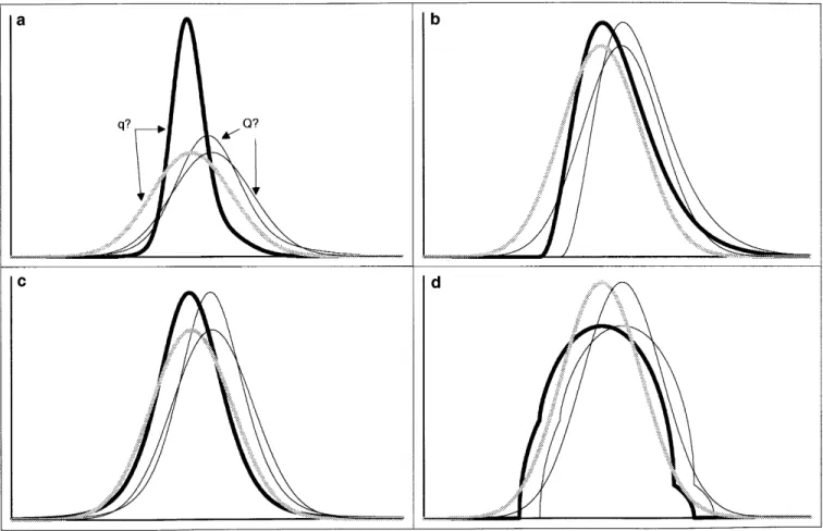
Figure 1.—Phenotypic distributions of offspring from heterozygous Qq sires, sorted according to the QTL allele inherited from the sire (Q or q), assuming (a) a heteroscedastic normal residual variance (r5 2; s 5 4); (b) a homoscedastic, skewed residual variance (x2
8); (c) a homoscedastic, positively kurtosed residual variance (t5); and (d) a homoscedastic, negatively kurtosed
residual variance (hemicircular residual variance). The phenotypic distributions of the q? offspring are shown (thick black lines) and compared with the corresponding distribution assuming a homoscedastic normal residual variance (thick gray lines). The corresponding distributions of the Q? offspring are shown as thin lines. Each class therefore comprises two subpopulations: QQ (25%) and Qq (75%) for the Q? class and Qq (25%) and qq (75%) for the q? class. The differences between the means of the
Q? and q? populations, corresponding to the effect of the Q to q allele substitution, equal 0.5sP.
described (Kappes et al. 1997) microsatellite markers from measuring of information content, and QTL mapping, were estimated from the dam population, separately for each pedi-bovine chromosome 6 (Table 2). Genotyping was performed
as described (Georges et al. 1995) or by using the “four dye- gree, as one lane” technology on an ABI373 or ABI377 sequencer.
p15 (1 2 p3) n11/(n111 n22)
Marker maps were built by using the CRIMAP program
p25 (1 2 p3) n22/(n111 n22)
(Lander and Green 1987) to determine the most likely order
p35 (n131 n23)/n.
and the ANIMAP program to refine the most likely
recombina-tion rates between adjacent markers (Georges et al. 1995). p1 and p2 correspond to the frequencies of two alleles from Information content along the marker map (Kruglyak and the sire, while p3 is the frequency of all other alleles pooled. Lander1995b) was measured as
nxycorresponds to the number of sons in the pedigree with
genotype xy, and n equals the total number of sons in the var[P(gi,A(s)|gi,L,gi,R)2 P(gi,B(s)|gi,L,gi,R)] pedigree.
5
o
ni51[P(gi,A(s)|gi,L,gi,R)2 P(gi,B(s)|gi,L,gi,R)]2n2 1 ,
RESULTS where n is the total number of sons in the granddaughter
Simulated data:Using the approach described in
ma-design (GDD).
QTL mapping was performed for five milk production traits: terials and methods,we simulated GDDs segregating
milk yield (kg), protein yield (kg), fat yield (kg), protein per- for a QTL explaining a fixed 9.4% of the phenotypic centage, and fat percentage. The phenotypes used for QTL variance (corresponding to a 5 0.5s
P) but with five
mapping were deviations of individual daughter yield
devia-alternative residual components: homoscedastic
nor-tions from the corresponding average of the parental
pre-mal, heteroscedastic norpre-mal, homoscedastic skewed,
ho-dicted transmitting abilities (Van Raden and Wiggans 1991).
nega-TABLE 1
Comparison of the power and precision of the RS and MR QTL mapping methods under five models of residual variance
Model 2 Model 1 (r5 2, s 5 4) Model 3 (x2 8) Model 4 (t5) Model 5(1⁄2o) RS MR RS MR RS MR RS MR RS MR Replicates 866 200 500 200 400 Average P value 0.24 0.23 0.19 0.22 0.20 0.23 0.20 0.25 0.25 0.21 12 b (a 5 0.05) 0.34 0.37 0.42 0.35 0.37 0.34 0.38 0.34 0.29 0.34 SD position (cM)a 24.1 22.6 27.1 24.3 21.7 22.8 20.2 20.4 22.1 21.1 RS vs. MRb P, 0.0001 P, 0.05 P, 0.001 P, 0.01 P, 0.0001 Model 1 vs. Model 3 (RS)c P, 0.01 P, 0.05 P, 0.05 P. 0.05 Model 1 vs. Model 3 (MR)c P. 0.05 P. 0.05 P. 0.05 P. 0.05
Model 1 is homoscedastic normal; 2, heteroscedastic normal; 3, homoscedastic skewed; 4, homoscedastic positively kurtosed; and 5, homoscedastic negatively kurtosed.
aStandard deviation of the most likely QTL position for all simulations with chromosome-wise P values less than 0.05. bComparison of P value distribution between methods, within models (Wilcoxon Matched Pairs Test).
cComparison of P value distribution between models, within methods (RS or MR, Mann-Whitney U test).
RS, rank-sum-based approach; MR, multipoint regression.
tive kurtosis. The generated datasets were all analyzed model (model 5; P5 0.000001); the loss of power with
the RS method was estimated at 14% ata-value of 0.05. by using both RS and MR methods. Table 1 reports, for
each of the five scenarios, the average P values and For the three remaining scenarios, however, the RS
approach outperformed MR, the gain in power ranging
the associated power at a-value of 0.05, obtained by
permutation as described in materials and methods. from 8 to 20% ata-value of 0.05 (Table 1).
The effect of the model on the power to detect the The relative merit of the RS and MR methods was
evaluated by using the Wilcoxon matched pairs test as QTL was evaluated by using the Mann-Whitney U test
(see materials and methods), by using model 1 as described in materials and methods. As expected,
multiple regression is superior to the rank-sum ap- reference. Comparisons were performed separately for
the RS and MR approach. Interestingly, MR appears to proach under the basic model of homoscedastic normal
residual variance (P 5 0.000014). The loss of power be quite insensitive to the nonnormality of the residual
variation, as the distribution of P values under the alter-when using the rank-based method is estimated at 8%
at a-value of 0.05. The MR method proved also signifi- native models is never significantly different from those obtained under the basic model. This is likely due to the cantly superior to the RS method in the negative kurtosis
TABLE 2
Primer pairs used for amplification of BTA6 microsatellite markers
u from previous
Marker UP-Primer (59–39) DN-Primer (59–39) marker
ILSTS090 TAGTACCATACCCAGGTAGG GCCAAAACACACAAGTGTGC 0
URB16 AGCTTTCTCTCACGGGTTTCG CGGACAGGACTGAGCTACTGA 0.219
BM1329 TTGTTTAGGCAAGTCCAAAGTC AACACCGCAGCTTCATCC 0.018
BM143 ACCTGGGAAGCCTCCATATC CTGCAGGCAGATTCTTTATCG 0.142
TGLA37 CATTCCAATCCCCTATCCTGAG TTGAATGATTCTATGAAGACCTGTA 0.061
ILSTS097 AAGAATTCCCGCTCAAGAGC GTCATTTCACCTCTACCTGG 0.105
BM4528 CAGAATCCATACACATGTCAACA AGGAACAGGTATAGGAATATTGGA 0.011
BM4621 CAAATTGACTTATCCTTGGCT TGTAATATCTGGGCTGCATC 0.033
RM028 CTACAGTCATGGGTCTGAAAG ATCTTCAGCCTGGCCTGAGAG 0.023
BM415 GCTACAGCCCTTCTGGTTTG GAGCTAATCACCAACAGCAAG 0.022
KCAS CAGTTACAAACATGTGGTGAGAATA AGAGCTTTGACATACAATAGACAA 0.079
ILSTS087 AGCAGACATGATGACTCAGC CTGCCTCTTTTCTTGAGAGC 0.030
BM4311 TCCACTTCTTCCCTCATCTCC GAAGTATATGTGTGCCTGGCC 0.011
BP7 GACCTTTTCACTGCCCTCTG TTTATTTCTGAGTCTTTGGGGC 0.018
Figure 2.—Information content (in percentage of the theoretical maximum) map along the length of bovine chromosome
6 when using (111) or ignoring (222) marker allele frequencies. Marker names and corresponding map position in
centi-morgans are shown along the x-axis.
fact that significance levels are deduced from phenotype covers 125 cM (Kosambi) with average interval of 9 cM.
The most likely order was in agreement with Kappes et permutations rather than from the theoretical
distri-bution of the test statistic. Using RS, on the contrary, al. (1996). The same figure also compares information
content when (1) exploiting marker allele frequency significant increases in detection power are observed for
models 2, 3, and 4 (respectively 9, 12, and 23% ata-value estimates to extract information from noninformative
marker genotypes, and (2) when ignoring this informa-of 0.05; Table 1), while the distribution informa-of P values does
not differ significantly between models 1 and 5. tion, i.e., when considering all microsatellite alleles to
be equally frequent in the population. It can be seen Estimates of the precision in the estimation of QTL
positions were also compared. Table 1 shows the that more than 80% of the maximal information is
ex-tracted for the central part of the chromosome; how-standard deviation of the most likely QTL position for
all simulations yielding a signal exceeding the 5% chro- ever, the information content drops at both extremities of the chromosome. Moreover, the figure shows that mosome-wise significant threshold. Comparing the
dif-ference between real and estimated position by using information content is improved only marginally by
con-sidering marker allele frequencies. This is especially true the Mann-Whitney U test, we found no evidence for a
significant effect either of the statistical method or of the in the central, denser part of the marker map.
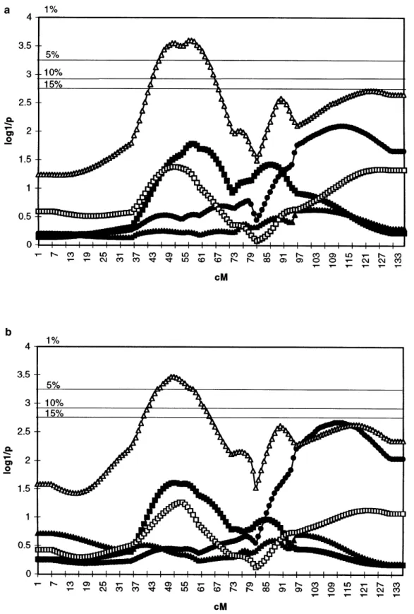
Figures 3a and 3b summarize the location score pro-model for the underlying residual variance. In essence,
precision was as poor in all circumstances, standard files obtained for the five different milk production
traits by using both RS and MR approaches. Generally deviations of the estimated position being 20 to 25 cM.
While the actual position of the QTL was at 62 cM speaking, both methods clearly yield very similar curves
for all traits along the entire chromosome length. For counting from the first marker, the estimates ranged
from 0 to 118 cM, i.e., the entire chromosome length. A protein percentage, the location scores maximize at the
same chromosome position (48 cM) using both ap-total of 95% of the estimates were within 43 cM (51.9 s)
from the actual position. proaches. The associated experiment-wise significance
levels are P5 0.03 for RS and P 5 0.01 for MR, therefore Real data:Table 2 and Figure 2 show the most likely
Figure 3.—Location scores obtained along chro-mosome 6 for milk (d), fat (m), and protein (j) yield, as well as fat (n) and pro-tein (h) percentage, using the RS (a) and MR methods (b). The y-axis corresponds to the log10of the inverse of
the corresponding chromo-some-wise P value as deter-mined by permutation. Ho-rizontal bars on the graphs correspond to 15, 10, 5, and 1% experiment-wise thresh-olds, obtained by applying a Bonferroni correction to the chromosome-wise sig-nificance levels.
These results are in agreement with the report of a corresponding pedigree material is given in Spelman
et al. (1996).
QTL affecting milk production on the centromeric half of chromosome 6, first identified by Georges et al. (1995) and later confirmed in independent studies in
DISCUSSION
Holstein-Friesian by Spelman et al. (1996) and Ku¨ hnet
al. (1996), in Finnish Ayrshire by Vilkki et al. (1997), In this article, we have adapted a nonparametric QTL mapping method based on sum of ranks that was de-and in Norwegian Red by Gomez-Raya et al. (1996).
and Lander 1995a) to outbred half-sib pedigrees. This method allows for missing genotypes in the “dams.” In such cases, estimates of marker allele frequencies can is particularly relevant for mapping QTL in specific
live-stock and plant species where such pedigrees routinely be used to improve inference about the identity of the
transmitted paternal chromosome. However, it is shown are generated within the context of specific breeding
designs. It extends the scope of QTL mapping in these that when performing multipoint analyses with dense
marker maps, this contributes only a marginal improve-pedigrees to a variety of not normally distributed traits,
including counts generated by a Poisson process, trun- ment of the information content. The benefit of
includ-ing marker allele frequency is therefore doubtful. In-cated data, and probabilities and qualitative data
(Krug-lyakand Lander 1995a). deed, errors in the estimation of the marker allele
frequencies may even cause an increase in type I errors We confirm that this approach (the RS method) can
be applied conveniently to normally distributed traits or a loss of power if accounting for inaccuracies in the
frequency estimates (Charlier et al. 1996). with minimal loss of power when compared to
paramet-ric methods. In the simulated example, we noticed a As expected, the precision in the estimation of the
QTL position using both proposed parametric and
non-loss of power of 8% ata-value of 5% when compared
to the MR method. When simulating nonnormal or parametric approaches is mediocre. This illustrates the
need to develop alternative strategies for fine-mapping heteroscedastic residuals, however, the RS method
out-performed the MR method in three out of four scenar- QTL in outbred populations.
ios (models 2–4: heteroscedastic normal, homoscedastic We acknowledge the financial support of Holland Genetics, Live-skewed, and homoscedastic positively kurtosed). Inter- stock Improvement Corporation, the Vlaamse Rundvee Vereniging, and the Ministe`re des Classes Moyennes et de l’Agriculture, Belgium.
estingly, this was shown not to be due to a loss of power
Continuous support from Nanke den Daas, Brian Wickham, Denis
of the MR approach, which proved to be relatively robust
Volckaert, and Pascal Leroy is greatly appreciated. We thank
in the scenarios that we simulated, but rather to a gain
Johan van Arendonk, Richard Spelman, Henk Bovenhuis,
of power when applying the RS method. Our interpreta- Marco Bink, Dave Johnson,and Dorian Garrick for fruitful
dis-tion of this finding is that in the three scenarios where cussions.
RS proved superior to MS, the phenotypic distribution is characterized by “outlyers” when compared to the
normal distribution (see Figure 1). These outlyers con- LITERATURE CITED
tribute excessively to the residual variation, while the
Charlier, C., F. Farnir, P. Berzi, P. Vanmanshoven, B. Brouwers
bulk of the observations actually are more centered et al., 1996 IBD mapping of recessive traits in livestock:
applica-tion to map the bovine syndactyly locus to chromosome 15.
Ge-around the mean (and therefore less variable) when
nome Res. 6: 580–589.
compared to the normal distribution. When using ranks
Churchill, G. A.,and R. W. Doerge, 1995 Empirical threshold
rather than the actual phenotypes, the contribution of values for quantitative trait mapping. Genetics 138: 963–971.
Cowan, C. W., M. R. Dentine, R. L. Axand L. A. Schuler, 1990
the outlyers to the residual variation is tempered,
there-Structural variation around prolactin gene linked to quantitative
fore increasing the ratio QTL variance/residual
vari-traits in elite Holstein sire family. Theor. Appl. Genet. 79: 577–
ance and concommitantly increasing the power to de- 582.
Falconer, D. S.,and T. F. C. Mackay, 1996 Introduction to
Quantita-tect the QTL.
tive Genetics. 4th Edition. Longman, New York. A disadvantage of the rank-based methods is the fact
Georges, M., D. Nielsen, M. Mackinnon, A. Mishra, R. Okimoto
that these do not provide convenient estimates of QTL et al., 1995 Mapping quantitative trait loci controlling milk
pro-duction by exploiting progeny testing. Genetics 139: 907–920.
effects. These methods therefore are suitable for the
Gomez-Raya, L., D. I.Va˚ ge, I. Olsaker, H. Klungland, G.
Klemets-detection of QTLs but have to be complemented with
dalet al., 1996 Mapping QTL affecting traits of economical
alternative methods, such as least-squares or maximum importance in Norwegian cattle. Proceedings of 47th Annual
Meeting of the European Association for Animal Production,
likelihood techniques when quantifying the QTL
ef-Lillehammer, Norway, August 25–29, 1996, p. 39.
fects.
Haley, C. S.,and S. A. Knott, 1992 A simple regression method
Recently, a number of QTL mapping methods that for mapping quantitative trait loci in line crosses using flanking
markers. Heredity 69: 315–324.
account for multiple linked or unlinked QTL have been
Hollander, M.,and D. A. Wolfe, 1973 Nonparametric Statistical
Meth-proposed. These include two QTL models (e.g., Haley
ods. John Wiley & Sons, New York.
and Knott 1992), composite interval mapping (Zeng Jansen, R. C.,1993 Interval mapping of multiple quantitative trait loci. Genetics 135: 205–211.
1993), and multiple QTL mapping ( Jansen 1993).
Kappes, S. M., J. W. Keele, R. T. Stone, R. A. McGraw, T. S.
Sonste-Rank-based approaches have been described to test
gardet al., 1997 A second-generation linkage map of the bovine
three or more classes, including the Kruskal-Wallis test genome. Genome Res. 7: 235–249.
Knott, S. A., J. M. Elsenand C. S. Haley, 1996 Methods for
multi-and the Jonckheere-Terpstra test, which would allow a
ple-marker mapping of quantitative trait loci in half-sib
popula-two-QTL model to fit. Alternatively, it might be
interest-tions. Theor. Appl. Genet. 93: 71–80.
ing to explore the possibility to use regression tech- Kruglyak, L.,and E. S. Lander, 1995a A nonparametric approach for mapping quantitative trait loci. Genetics 139: 1421–1428.
niques directly on ranks, which, if applicable, would
Kruglyak, L.,and E. S. Lander, 1995b Complete multipoint
sib-allow inclusion of additional markers as cofactors in the
pair analysis of qualitative and quantitative traits. Am. J. Hum.
model. Genet. 57: 439–454.
Ku¨ hn, Ch., R. Weikard, T. Goldammer, S. Grupe, I. Olsakeret
al., 1996 Isolation and application of chromosome 6 specific Weber, J. L.,and P. E. May, 1989 Abundant class of human DNA microsattelite markers for detection of QTL for milk-production polymorphisms which can be typed using the polymerase chain traits in cattle. J. Anim. Breed. Genet. 113: 355–362. reaction. Am. J. Hum. Genet. 44: 388–396.
Lander, E. S.,and P. Green, 1987 Construction of multilocus ge- Weller, J. I., Y. Kashiand M. Soller, 1990 Power of daughter and netic linkage maps in humans. Proc. Natl. Acad. Sci. USA 84: granddaughter designs for determining linkage between marker 2363–2367. loci and quantitatve trait loci in dairy cattle. J. Dairy Sci. 73: Spelman, R. L., W. Coppieters, L. Karim, J. A. M. van Arendonk 2525–2537.
and H. Bovenhuis, 1996 Quantitative trait loci analysis for five Williams, J. G., A. R. Kubelik, K. J. Livak, J. A. Rafalskiand S. V. milk production traits on chromosome six in the dutch Holstein- Tingey,1990 DNA polymorphisms amplified by arbitrary prim-Friesian population. Genetics 144: 1799–1808. ers are useful as genetic markers. Nucleic Acids Res. 18: 6531– Van Raden, P. M.,and G. R. Wiggans, 1991 Derivation, calculation,
6535.
and use of National Animal Model Information. J. Dairy Sci. 74: Zeng, Z-B.,1993 Theoretical basis of separation of multiple linked 2737–2746. gene effects on mapping quantitative trait loci. Proc. Natl. Acad. Vilkki, H. J., D.-J. de Koning, K. Elo, R. Velmalaand A.
Maki-Sci. USA 90: 10972–10976. Tanila, 1997 Multiple marker mapping of quantitative trait
loci of Finnish dairy cattle by regression. J. Dairy Sci. 80: 198–204. Communicating editor: Z-B. Zeng Vos, P., R. Hogers, M. Bleeker, M. Reijans, T. van de Leeet al.,
1995 AFLP: a new technique for DNA fingerprinting. Nucleic Acids Res. 23: 4407–4414.